Abstract
A novel technique named Signal Analysis based on Chaos using Density of Maxima (SAC-DM) is presented to analyze Brushless Direct Current (BLDC) motors behavior. These motors are vastly used in electric vehicles, especially in Drones. The proposed approach is compared with the traditional Fast-Fourier Transform (FFT) and the experiments analyzing a BLDC motor of a drone demonstrates similar results but computationally simpler than that. The main contribution of this technique is the possibility to analyze signals in time domain, instead of the frequency domain. It is possible to identify working and faulty behavior with less computational resources than the traditional approach.
1. Introduction
Considering the growth in the application of Unmanned Aerial Vehicles (UAV) systems around the world [1,2,3], it is mandatory the research and development of safe and reliable solutions [4,5]. The motors used in UAV must receive more attention as possible. Brushless Direct Current (BLDC) motors are formed by synchronous generators with permanent magnets and stationary armatures. It has rotating magnets with magnets axially facing the armatures, e.g., hub-type cycle dynamos [6]. They are vastly used by industry in machines, e.g., [7], and as the main alternative for electrical vehicles such as commercial UAV [8,9,10].
There are some possible causes of failures in BLDC motors, like stator, rotor, bearing and inverter faults [11], and many approaches to implement fault tolerant aerial vehicles. Solomon [9] shows that the speed control scheme primarily made up of standard proportional integral controllers presented loss of altitude and exacerbate thrust when the system was operated in speed control mode. Thus, he proposes a new solution based on Model Reference Adaptive Control (MRAC) to improve the speed control and improvement in flight performance of the UAV system.
In [10], the authors study a solution to control of permanent magnet synchronous motors (PMSM) instead of BLDC. However, it shows interesting concepts as the difference between sinusoidal and trapezoidal back EMF; Extend Kalman Filter (EKF) and Sliding Mode Observer (SMO). It is an efficient approach, however, the usage of filter adds computational complexity to the analysis. Our approach does not require filters for the analysis of electrical current signal.
Other authors investigate the analysis and diagnosis of Brushless Direct Current (BLDC) motors. The work from Hou et al. [12] proposes the use of Local Polynomial Fourier Transform (LPFT) to perform the Motor Current Signature Analysis (MCSA) to detect failures in BLDC motors. In [7], the authors analyze operating characteristics of BLDC motors and propose a simple fault diagnosis system. All these solutions analyze the signal in frequency domain, which requires an extra computational effort, while our approach is based on the analysis in time domain.
Here, we propose a technique named Signal Analysis based on Chaos using Density of Maxima (SAC-DM) to analyze Brushless Direct Current (BLDC) motors generally used in Drones. This technique demonstrated potential to characterize motors with a simple computational approach from the electric current signal, enabling its application in time-critical applications (presented in Section 2). The characterization tested in the experiments here is the detection of the loose stator and the rotation direction, though other characterization would also be possible, e.g., speed detection, unbalanced propeller identification and out-of-order vibration.
The proposed approach presented here applies ideas developed in nuclear physics, quantum transport in nanostructures and biological systems [13] to study the characteristics of Brushless Direct Current (BLDC) used in drones. Recent experimental applications of the method include the study of chaotic dynamics in electromagnetic resonant cavities that may serve to cryptography, emulated quantum entanglement, etc. [14] and chaos study in biological systems [13], but in this paper, we present a novel signal analysis method to characterize the chaos in BLDC motors of drones.
Two contributions are presented in this paper: (i) to demonstrate that the same behavior detected from current signal of Brushless Direct Current (BLDC) motors using FFT could also be captured from the chaotic behavior of the system; (ii) to propose a novel approach to determine the chaotic behavior of BDLC motors from the correlation coefficient based on density of maxima.
At first, The SAC-DM approach is presented (Section 2). To demonstrate its potential, an experiment is presented where a small BLDC motor with a propeller is tested in different conditions (Section 3). The results of the proposed technique are compared with two traditional approaches: Fast-Fourier Transform (FFT) and analysis of chaos calculating the length at half-height from the auto-correlation function (see Section 4). The results with SAC-DM are demonstrated is Section 5 and present the equivalence of the proposed approach with the traditional ones, demonstrating its potential for signal analysis in general. Final considerations are presented in Section 6.
2. Signal Analysis using Chaos based of Density of Maxima (SAC-DM)
In previous work, it was demonstrated that the number of maxima can be related to the correlation length, due to the intrinsic chaotic behavior of the density of individuals in a bio-diversity scenario [13]. The cyclic equilibrium behavior is the central issue of that work and is used to identify the chaotic behavior even in a single and short time of the system, as it is assured by the maximum entropy principle and the ergodic theorem.
Using the maximum entropy principle and extensions of chaos theory, we propose a procedure for characterizing the chaos in brushless motors analyzing a generic amount . Our solution solves the problem of how to characterize problems featuring a small amount of data and identifies the presence of chaos in seemingly random series of information .
The signal evolves in time and fluctuates to produce local maximum in the interval , for sufficiently small , so one has and where prime stands for the time derivative, such that, . The joint probability can be used to calculate the average density of maxima through the simple route: the probability to find a maximum in the interval is proportional to the integral spanning the region defined above, such that
The fact that the statistical properties of the mean number of peaks are invariant under time translations indicates that both and have vanishing average values. Moreover, the properties of can be obtained from the smallest momenta of and , and the variances of are directly related to the correlation function
We can then obtain the several momenta, in particular
The principle of maximum entropy can be used to construct the joint probability distribution for and its derivatives from the previous equations. After implementing the algebraic calculations, integration on leads to which gives
The main results are shown in the previous Equations and can be used to write in the form
Due to the chaotic properties of stochastic systems, the approach was reduced to obtain the correlation length as a simple formula that considers only the density of maxima of the original signal. Using Equations (3) and (5) for periodic functions, the normalized correlation function can be written in terms of a cosine function and allows us to reduce it to a very simple equation relating the correlation length with the simple density of maxima as follows
where is the correlation length and is the density of maxima.
This result offers a new quantity that arises from the chaotic behavior imprinted in the stochastic data. This method calculates the average of the density of maxima of the samples. It allows us to estimate properties of a system even when a unique and short temporal series is available and to estimate the correlation coefficient.
3. Experimental Scenarios
In practice, current sensors measure the stator current of BLDC motor for a one electrical degree rotation.
A three-phase BLDC motor testbench designed for electric motor application is used as a practical test motor. Experimental setup of BLDC motor that is used to validate simulation model is shown in Figure 1.
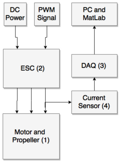
Figure 1.
Testbench represantation.
It is formed by (1) Brushless DC Motor with a propeller; (2) Electronic Speed Controller (ESC); (3) National Instruments (NI) Data Acquisition Device (DAQ) model USB 6215; (4) Current sensor. The Data Acquisition device has been used to test the technique. Actually, a system is being developed to be embedded in drones for real-time data acquisition and diagnosis.
The specification of the BLDC motor is presented in Table 1, which was used in four different execution, as can be seen in Table 2.

Table 1.
BLDC Motor Specifications.
Table 2.
Experimental scenarios.
Using 2 different motors (one being defective) and one propeller rotating in the clockwise (CW) and counterclockwise (CCW) directions. Motor 1 is in perfect conditions and motor 2 is defective due to the loose stator. For each scenario, 1,000,000 samples were collected at a rate of 10,000 samples per second. All scenarios running at constant speed at 600 rpm.
4. Signal Analysis Using Traditional Approaches
In this section, the results are analyzed using two traditional approaches. First, using Fast Fourier Transform (FFT) and then using the analysis of chaotic behavior using the Correlation Length Coefficient (CLC). After that, In Section 5 is possible to compare these results with SAC-DM results.
4.1. Fast Fourier Transform (FFT)
In the first stage of the experiment, the signal was collected through the current sensor connected to one of the phases of the motor. Figure 2 presents one example of a signal acquired for each scenario. The signals are presented in Amperes. As can be seen, there is some difference in phase among the signals due to minimal differences in fundamental, or main frequency, as presented as following.
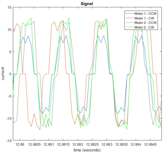
Figure 2.
Stator Current signal from each scenario.
In this chart, it is possible to observe that the acquired signal presents trapezoidal characteristics and a phase difference between the scenarios, due to the essence of the BLDC motors, and some amplitude reduction for scenario S1 (motor1-CCW)
Once the data were collected and analyzed in the time domain, they were submitted to a Fast Fourier Transform (FFT) for analysis in the frequency domain. The signals in the frequency domain for each scenario are shown in Figure 3.
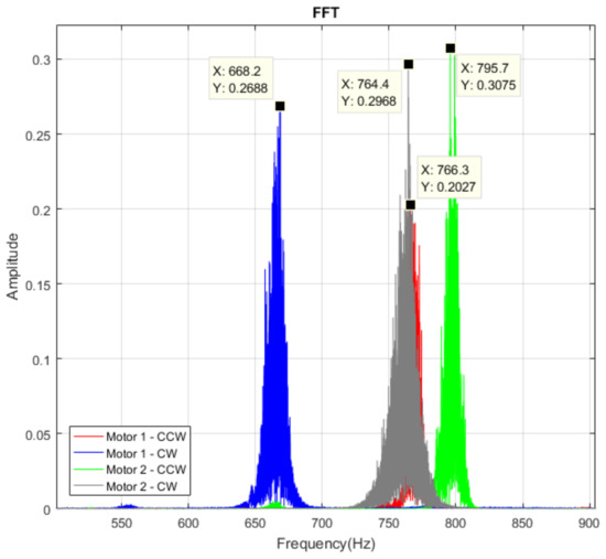
Figure 3.
Signals of all scenarios in the Frequency Domain.
The signal in frequency demonstrates that the fundamental, or main frequency of scenarios S1 (motor1-CCW) and S4 (motor2-CW) are similar, with 766.3 Hz and 764.4 Hz, respectively. The scenario S3 also presents a similar fundamental frequency, with 795.7 Hz. The value for Scenario S2 is less similar, with 668.2 Hz.
As expected, characteristics of the system (propeller, rotation, and defect in motors) might result in changes in the fundamental frequency of the current signal. These results will be used as a reference to the approach proposed in this work, where the characteristics of the system are analyzes based on the chaotic behavior of the signal.
4.2. Correlation Length Coefficient (CLC)
As an alternative to analysis using FFT, we apply the chaotic behavior analysis method using the correlation probability, which uses the initial correlation coefficient of the signal as a measure to quantify the chaotic behavior of the system. This technique is based on the fact that chaotic systems auto-correlate over time, different from random systems, which autocorrelation function tends to not converge.
For a signal which represents a stationary process with the mean and variance , and its covariance only depend on time difference .
To illustrate the computation of the samples using the Auto-correlation Function, consider the following distribution of the signal . Where the time ; and represents the quantity of samples at each time. Organizing the values of per line in a matrix, we have M:
Thus, the auto-correlation function (ACF) of the signal is defined as [15]:
Applying the matrix M (7) in the function (8), we have the Auto-correlation matrix as result. However, to calculate the Correlation Length Coefficient (CLC) it is necessary to calculate the Partial Auto-correlation Function (PACF).
For this, first it is calculated as the best linear estimation in the mean square sense of :
where with is the mean squared linear regression coefficient. Then, the correlation condition is called the Partial Auto-correlation Function (PACF), denoted as .
Finally, the process returns the autocorrelation function () as shown in Figure 4. The descending amplitude of the autocorrelation function during the time is an expected behavior from chaotic periodic systems.
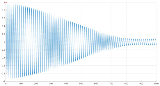
Figure 4.
PACF computation result.
Figure 5 presents the autocorrelation function presented in Figure 4, but only for X from 1 to 3.5. To prove that the system is chaotic, the length at half-height is calculated from . Considering the points and B has in Figure 5. This value is called Correlation Length Coefficient (CLC) , where:
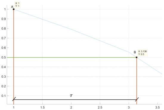
Figure 5.
Correlation Length.
The system can be considered chaotic if observed in the autocorrelation function (Figure 5) is the same as the obtained counting the density of maxima and applying Equation (6). In Figure 5 the observed value is .
The Correlation Length Coefficient obtained using the half-height technique (observed from autocorrelation function) are presented in Table 3. It presents the correlation coefficients obtained from 4 different executions (E) for each of all scenarios(S). In addition, it presents the mean (), variance() and standard deviation() of the obtained results.
Table 3.
Correlation Length Coefficients (CLC).
The first contribution of this work is to demonstrate that the same behavior detected using FFT could be captured from the chaotic behavior of the system. From FFT it was presented that the fundamental frequency of scenario S1 is similar to S4, which are 766.3 Hz and 764.4 Hz (see Figure 3), respectively. Scenario S3 is also not so different, with 795.7 Hz. The scenario with a greater difference in its fundamental frequency is S2, with 668.2 Hz. From Table 3 it is possible to see the same pattern. S1 and S4 have the more similar correlation length coefficient calculated, which are about 2.087 and 2.116, respectively. Similar to FFT, S3 has a coefficient close the ones from S1 and S4, with 2.045. Also, S2 was the scenario with a more distant coefficient, with about 2.393. It important to note that the fundamental frequency in FFT and the correlation coefficient are inversely proportional.
Though the method is efficient to detect some anomalies in the system, a large amount of data is necessary and the computing cost to calculate the correlation function is high. As an alternative, we propose the application of a novel approach to calculate the correlation coefficient based on the density of maxima, which is the second and main contribution of this paper.
5. Results with SAC-DM
The same data used in Section 4 was reused to identify faulty behavior and validate the SAC-DM approach, now using the Equation (6). The same behavior detected with traditional Correlation Length Coefficient (CLC) approach (Table 3) was captured by the SAC-DM method, as presented in Table 4. In addition, It presents the mean (), variance() and standard deviation() of the obtained results.
Table 4.
SAC-DM - 1,000,000 samples.
Although the values are not same, the behaviors detected with FFT and Correlation Length Coefficient (CLC) are maintained with SAC-DM. That is, scenario S2 has the highest value, followed by S4, S1, and S3 (in FFT this order is inverse).
It is also possible to see that with SAC-DM the same similarities with FFT are detected, as presented in Table 5, sometimes with results even more similar to FFT than the ones obtained using length at half-height, e.g., in SAC-DM the relation between scenarios S3 and S4 with S2 are more similar with FFT than in Correlation Length Coefficient (CLC).
Table 5.
Relation between the FFT, Correlation Length Coefficient (CLC) and SAC-DM.
This result is important because it demonstrates that SAC-DM returns values equivalent to the ones produced by the approach based on Correlation Length Coefficient (CLC). However, the SAC-DM processes the original signal without any filtering, and the second approach obtains the coefficient from the autocorrelation function, which is computationally much more expensive than the density of maxima.
The similarities between FFT, CLC, and SAC-DM are clearer when seeing the values of each scenario in comparison with S2 (scenario with lowest fundamental frequency in FFT). This comparison can be seen in Table 5. The fundamental frequency in FFT of each scenario is divided by the value of scenario S2. The FFT is inversely proportional to correlation length, the value of S2 is divided by the ones from each scenario collected using CLC and SAC-DM. The values demonstrate that using SAC-DM, even with no identical values in comparison with CLC, the essential characteristics of the signals are preserved.
In order to evaluate the behavior of SAC-DM along the time, the correlation coefficient was calculated for every 1000 values for the whole dataset with 1,000,000 samples, resulting in 1000 SAC-DM coefficients as result, as shown Table 6.
Table 6.
SAC-DM for 1000 samples.
These results are presented in Figure 6. The probability distribution is Gaussian for all four scenarios, with lower Variance in scenarios S1 and S2, and higher in S3 and S4.
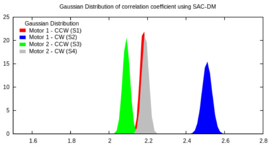
Figure 6.
Gaussian distribution of correlation coefficient using SAC-DM for scenarios S1 (red), S2 (blue), S3 (green) and S4 (gray).
This analysis demonstrates another important feature of the proposed SAC-DM approach. The correlation coefficient calculated with our approach is distributed following a Gaussian distribution with low variance, which means even few values (1000 in this case) are enough to generate a correlation coefficient similar to those ones calculated using the length at half-height using 1 million values and input. This turns SAC-DM into an approach even less computationally intensive than FFT and CLC.
6. Conclusions
The main contribution of this paper is to propose the application of the density of maxima to analyze Brushless Direct Current (BLDC) motors commonly used in Drones by the electrical current signal from the stator. This approach is called Signal Analysis using Chaos based on Density of Maxima (SAC-DM), which describes a simplification to obtain the correlation coefficient of stochastic functions.
In this work, the SAC-DM approach was demonstrated to efficiently characterize brushless motors, when through the signal of electric current of the stator it is possible to differentiate the behavior of the motor between the working and the faulty condition. The innovative method proved to achieve similar results as Fast-Fourier Transform but using a shorter amount of data and lesser calculation. Due to the low demand for computing resources, this opens the possibility to apply this technique also to diagnose Brushless Motors in real-time using a simple micro-controller. This new application is being investigating for future works.
Author Contributions
For the elaboration of this work, Jorge Ramos, Abel Lima Filho and Tiago Nascimento were responsible for the theoretical and mathematical background. Ramon Medeiros contributed with the experiments, analysis and writing. Alisson Brito was the coordinator of the work and reviewed the text.
Conflicts of Interest
The authors declare no conflict of interest.
References
- Kuzma, J.; O’Sullivan, S.; Philippe, T.; Koehler, J.; Coronel, R. Commercialization Strategy in Managing Online Presence in the Unmanned Aerial Vehicle Industry. Int. J. Bus. Strateg. 2017, 17, 59–68. [Google Scholar] [CrossRef]
- Stöcker, C.; Bennett, R.; Nex, F.; Gerke, M.; Zevenbergen, J. Review of the Current State of UAV Regulations. Remote Sens. 2017, 9, 459. [Google Scholar] [CrossRef]
- Mills, M.P. Drone Disruption: The Stakes, The Players, And The Opportunities. 2017. Available online: https://www.forbes.com (accessed on 20 March 2017).
- Yuan, Y.; Yuan, H.; Guo, L.; Yang, H.; Sun, S. Resilient Control of Networked Control System under DoS Attacks: A Unified Game Approach. IEEE Trans. Ind. Inform. 2016, 12, 1786–1794. [Google Scholar] [CrossRef]
- Xiao, B.; Yin, S. A New Disturbance Attenuation Control Scheme for Quadrotor Unmanned Aerial Vehicles. IEEE Trans. Ind. Inform. 2017, 13, 2922–2932. [Google Scholar] [CrossRef]
- Lopatinsky, E.; Schaefer, D.; Rosenfeld, S.; Fedoseyev, L. Brushless DC Electric Motor. U.S. Patent 7,112,910, 26 September 2006. [Google Scholar]
- Park, B.G.; Lee, K.J.; Kim, R.Y.; Kim, T.S.; Ryu, J.S.; Hyun, D.S. Simple Fault Diagnosis Based on Operating Characteristic of Brushless Direct-Current Motor Drives. IEEE Trans. Ind. Electron. 2011, 58, 1586–1593. [Google Scholar] [CrossRef]
- Tefay, B.; Eizad, B.; Crosthwaite, P.; Singh, S.; Postula, A. Design of an integrated electronic speed controller for agile robotic vehicles. In Proceedings of the Australasian Conference on Robotics and Automation (ACRA 2011), Melbourne, Australia, 7–9 December 2011. [Google Scholar]
- Solomon, O. Model Reference Adaptive Control of a Permanent Magnet Brushless DC Motor for UAV Electric Propulsion System. In Proceedings of the IECON 33rd Annual Conference of the IEEE Industrial Electronics Society, Taipei, Taiwan, 5–8 November 2007; pp. 1186–1191. [Google Scholar]
- Koteich, M.; Moing, T.L.; Janot, A.; Defay, F. A real-time observer for UAV’s brushless motors. In Proceedings of the IEEE 11th International Workshop of Electronics, Control, Measurement, Signals and their application to Mechatronics, Toulouse, France, 24–26 June 2013; pp. 1–5. [Google Scholar]
- Baek, G.; Kim, Y.; Kim, S. Fault diagnosis of identical brushless DC motors under patterns of state change. In Proceedings of the IEEE International Conference on Fuzzy Systems (IEEE World Congress on Computational Intelligence), Hong Kong, China, 1–6 June 2008; pp. 2083–2088. [Google Scholar]
- Hou, W.; Zhang, Y.; Sun, J. A fault detection method for motors based on Local Polynomial Fourier Transform. In Proceedings of the Prognostics and System Health Management Conference (PHM), Beijing, China, 21–23 October 2015; pp. 1–5. [Google Scholar]
- Bazeia, D.; Pereira, M.; Brito, A.; de Oliveira, B.; Ramos, J. A novel procedure for the identification of chaos in complex biological systems. Sci. Rep. 2017, 7, 44900. [Google Scholar] [CrossRef] [PubMed]
- Dietz, B.; Richter, A.; Samajdar, R. Cross-section fluctuations in open microwave billiards and quantum graphs: The counting-of-maxima method revisited. Phys. Rev. E 2015, 92, 22904. [Google Scholar] [CrossRef] [PubMed]
- Wei, W.W.S. Time Series Analysis: Univariate and Multivariate Methods; Pearson: London, UK, 2006. [Google Scholar]
© 2018 by the authors. Licensee MDPI, Basel, Switzerland. This article is an open access article distributed under the terms and conditions of the Creative Commons Attribution (CC BY) license (http://creativecommons.org/licenses/by/4.0/).