Dual-Channel Induced Countermeasure Strategy for Formation Control of Distributed UAV Swarms with Prescribed Flight Trajectory

Highlights

What are the main findings?

• A novel dual-channel induced countermeasure protocol is proposed for the distributed UAV swarm, and a closed-form expression for the countermeasure flight trajectory is derived.
• A necessary and sufficient condition for the feasibility of the DCICS is established, and design criteria for the countermeasure signals are derived under a robust $H_{\infty }$ performance framework.

What are the implications of the main findings?

• The proposed strategy enables directional and controllable eviction of the malicious distributed UAV swarm while maintaining the original formation structure, offering a non-destructive countermeasure paradigm for civilian low-altitude security.
• By increasing the number of injection channels for the countermeasure signals, the proposed strategy expands the feasible set of the countermeasure flight trajectory and applies to a broader range of civilian UAV swarm countermeasure scenarios.

Abstract

For malicious distributed unmanned aerial vehicle (UAV) swarms operating in civilian airspace, this paper proposes a novel dual-channel induced countermeasure strategy (DCICS) with prescribed countermeasure flight trajectories, in which the designable countermeasure signals are injected into the sensor–controller (SC) channel and the controller–actuator (CA) channel of partial or all UAVs, simultaneously. Firstly, we establish a dual-channel induced countermeasure protocol, in which the sensor-induced countermeasure signal is modeled as a continuous function of swarm dynamics, whereas the actuator-induced countermeasure signal is generated through a countermeasure signal generation exosystem (CSGES). Then, we derive a closed-form expression of the countermeasure flight trajectory, explicitly characterizing the effect of the countermeasure signals on the swarm motion. Furthermore, a necessary and sufficient condition for the feasibility of the DCICS is derived. By introducing adjustable performance factors, we construct a robust $H_{\infty }$ framework and provide the design criteria for the dual-channel induced countermeasure signals accordingly. The proposed strategy can drive the formation of the distributed UAV swarm along a prescribed countermeasure flight trajectory while maintaining the original formation structure. Finally, we present numerical simulation examples to validate the effectiveness of the theoretical results.

1. Introduction

In recent years, the rapid development of the civilian low-altitude economy has led to an explosive growth in the deployment of distributed UAV swarms for civilian applications [1]. By leveraging distributed interaction mechanisms and cooperative control protocols, the swarm can autonomously form and maintain desired formation structures to accomplish complex missions such as emergency search, agricultural monitoring, and infrastructure inspection [2,3]. Research on UAV energy consumption has further enhanced the endurance and operational capability of UAVs, and enabled UAVs to undertake longer-duration and more complex tasks across diverse operational environments [4,5,6]. In networked UAV operations, path planning is critical to mission execution efficiency, while advances in autonomous navigation and communication technologies have significantly enhanced the cooperative capabilities of UAV swarm systems [7]. Meanwhile, the increasing maturity of swarm control technologies has posed serious threats to civilian infrastructure and airspace management, and has also hindered the development of the low-altitude economy. Confronted with security threats launched by malicious UAVs, the development of countermeasure technologies has lagged behind that of swarm control technologies. Consequently, it is urgently necessary to develop effective countermeasure approaches to safeguard civilian airspace security and protect the development of the low-altitude economy.

According to the form of countermeasures, the current swarm countermeasure technologies can be classified into physical countermeasures, electromagnetic countermeasures, and swarm confrontation [8]. Physical countermeasures directly target the physical structure of UAVs, damaging critical components to undermine the cooperative effectiveness of the swarm [9]. Electromagnetic countermeasures aim to disrupt the command and control links or navigation systems of UAVs and impair the swarm cooperative performance without physical contact [10]. Swarm confrontation employs a countermeasure UAV swarm to engage in aerial adversarial games against the malicious swarm, conducting strikes through impacts and area jamming [11]. Xing et al. [12] presented a comprehensive survey of counter-UAV technologies, covering a wide range of detection methods and providing detailed discussions on defensive countermeasures, including directed-energy weapons, electronic jamming, and swarm confrontation. They emphasized that counter-UAV technology is evolving toward the integrated deployment of multiple countermeasure strategies. However, these approaches exhibit low cost-effectiveness in dealing with the distributed UAV swarm. Furthermore, Xing et al. [13] investigated safe motion planning and multi-task coordination for complex robotic systems, proposing an optimization framework based on hierarchical quadratic programming. This multi-constraint optimization paradigm bears direct relevance to the countermeasure strategies. Meanwhile, Yu et al. [14] provided a comprehensive review of UAV formation control from a task-driven perspective, offering novel methodological insights into swarm countermeasure problems. As a typical multiagent system, the distributed network is the key to achieving cooperative formation for the distributed UAV swarm. Morshedi et al. [15] presented a systematic survey of cybersecurity threats facing UAVs and pointed out that the reliance of UAVs on open wireless communication channels renders them highly vulnerable to cyber attacks. Similarly, Umrani et al. [16] highlighted the possibility of exploiting weaknesses in UAV sensing and estimation functions, demonstrating that injecting false signals consistent with the internal logic can effectively drive the swarms away without triggering their detection or defense mechanisms. Consequently, cyber-based countermeasures that exploit vulnerabilities in distributed interaction networks have emerged as a new research direction for swarm security [17].

Based on the implementation mechanisms, cyber-based countermeasure approaches are classified as Denial of Service (DoS) attack-based and deception attack-based countermeasure approaches. DoS attacks achieve swarm countermeasure objectives by transmitting massive junk data packets to occupy channel resources, which can block information interaction among UAVs and incapacitate UAVs from conducting timely feedback control based on state information of neighbors [18]. Sun et al. [19] developed a periodic DoS attack with a fixed attack frequency, which can block all interaction channels of the system. Random DoS attack strategies were proposed in [20,21], where attack signals followed the Bernoulli distribution and the Markov process. In practical countermeasure scenarios, countermeasure approaches are typically implemented under the condition of bounded energy. In [22], an energy-constrained DoS attack model was proposed, where the attack energy was constrained by limiting the attack frequency and the total attack duration. Beyond full-channel DoS attacks, Li et al. [23] proposed a data-importance-aware DoS attack strategy with partial channel blocking, which improved attack stealthiness while reducing the consumption of attack resources. It should be noted that although DoS attacks can disrupt the cooperative performance, the attack process is prone to triggering the attack detection and defense mechanisms of the swarm [24].

Deception attacks compromise the integrity of swarm interaction information by injecting deception signals to tamper with the state perception or control input of UAVs [25]. For the SC channel, Yuan et al. [26] designed an innovation-based sensor deception attack strategy by fusing wireless measurement data with the system state information. Regarding the CA channel, a time-varying function attack model and a full-state-based attack model were developed for multiagent systems in [27,28], respectively. Li et al. [29] designed an attack model that was described by a stochastic inverse dynamics function and does not rely on time-varying functions or system states. In addition, a joint attack strategy was proposed in [30], which can simultaneously attack both the SC channel and the CA channel of the swarm system. In [31], a dual-channel random switching deception attack strategy was proposed, which not only saved attack resources but also further increased the difficulty of system detection and defense. It should be noted that the aforementioned studies achieve the weakening of the system performance by disrupting the cooperative behaviors. However, the disruption of the cooperative behaviors may lead to the loss of control of UAVs and consequently cause even more severe secondary damage to civilian infrastructure and human lives.

Unlike the destructive behaviors of the aforementioned attack-based countermeasure approaches, induced attack-based countermeasure approaches are intended to make the swarm fly along a countermeasure trajectory prescribed while maintaining system stability, which means achieving the directional and controllable expulsion of the distributed UAV swarm, as described in [32]. From a civilian-benefit perspective, the induced countermeasure approach offers non-destructive and controllable solutions that can reduce secondary damage in populated environments, thereby protecting civilian infrastructure and human lives. The induced countermeasure can be classified into the sensor-induced countermeasure and the actuator-induced countermeasure, and countermeasure signals are injected into the SC channel and the CA channel of UAVs, respectively. Regarding the sensor-induced countermeasure, a general design approach of attacks against the multiagent system was proposed in [33] based on the internal model principle. In [34], a displacement attack strategy was designed for the formation control protocol of multiagent systems, which can hijack the system to the predetermined countermeasure area. To address the issue of swarm disorder during the countermeasure process, Geng et al. [35] developed a swarm countermeasure approach based on the Global Navigation Satellite System that targets the sensors of UAVs. In [36], a sensor-based countermeasure strategy was proposed for a quadrotor swarm, which saved countermeasure resources while achieving directional eviction for the swarm. For the CA channel of UAVs, Li et al. [37] proposed an actuator-based induced attack that can prescribe the induced trajectory. In [38], an induced attack protocol was constructed by integrating the attack model among agents and dynamic event-triggered techniques.

According to the working principles of UAVs, the SC channel requires receiving navigation information. The sensor-induced countermeasure strategy exploits the openness and injects the countermeasure signal through navigation spoofing. Consequently, the implementation of the sensor-induced countermeasure strategy is relatively straightforward. However, the state estimators can detect and correct abrupt changes in perceived states. Therefore, the sensor-induced countermeasure strategy lacks sufficient stealthiness [39]. Compared with the sensor-induced countermeasure strategy, the actuator-induced countermeasure signal is injected into the channel between the state estimator (inside the controller) and the actuator, which can promptly cover the correct signals [40]. Hence, the actuator-induced countermeasure strategy possesses better stealthiness. However, due to the closed nature of the CA channel, the injection of the actuator-induced countermeasure signal can only be realised through electromagnetic interference (EMI) [8], but the success rate of the signal injection is relatively low. Evidently, both induced countermeasure strategies have limitations in practical applications, and a certain complementary relationship exists between the sensor-induced countermeasure strategy and the actuator-induced countermeasure strategy. Unfortunately, existing studies have not yet considered a joint induced countermeasure strategy that simultaneously targets both the SC channel and the CA channel.

In parallel with the aforementioned countermeasure strategy studies, risk assessment methods have also been applied to evaluate the vulnerability of UAVs to cyber-based countermeasure approaches. Bozveliev et al. [41] proposed a risk assessment framework for UAV cyber attacks based on intuitionistic fuzzy estimation, enabling qualitative evaluation of cyber risks. However, such approaches focus on vulnerability identification and risk quantification rather than active intervention, and therefore cannot provide a viable solution for swarm countermeasures. This paper aims to design a novel induced countermeasure strategy from the civilian defensive perspective to reduce the impact of the distributed UAV swarm on civilian airspace security and management. The designed countermeasure signals are injected into the SC and CA channels of partial or all UAVs and diffused throughout the swarm through the distributed interaction protocol, which enables the swarm to fly along the countermeasure flight trajectory designed while maintaining formation stability. Compared with the multi-channel attack strategy proposed in [42] and the coordinated attack strategy presented in [43], the proposed DCICS differs fundamentally in theoretical modeling, control objectives, and practical implementation. In terms of theoretical modeling, both [42,43] model attack signals as independent adversarial inputs with stochastic characteristics, whereas the proposed protocol establishes an explicit causal relationship for the countermeasure signals by designing a CSGES. Regarding control objectives, whereas existing studies primarily seek to disrupt system stability or consensus, the proposed strategy aims to achieve directed and controllable induced countermeasure for the swarm while maintaining the original formation structure. In practical implementation, unlike the abstract modeling adopted in prior works, the proposed strategy integrates navigation deception on the SC channel and EMI for the CA channel, thereby providing a concrete and actionable dual-channel injection mechanism for the distributed UAV swarm. The main contributions of this paper are as follows.

• This paper proposes a novel DCICS that acts on the sensors and actuators of partial or all UAVs. We develop a dual-channel induced countermeasure protocol for the swarm, which improves the success rate of countermeasure signal injection and simultaneously ensures excellent stealthiness. The proposed strategy subsumes the single-channel induced attacks discussed in [36,37,38,40] as special instances.
• Different from [32,33,34,35], this paper provides an explicit closed-form expression of the countermeasure flight trajectory, which can be altered by designing the dual-channel induced countermeasure signals. Moreover, compared with [36,37,38], the DCICS expands the designed feasible set of the countermeasure flight trajectory.
• We derive a necessary and sufficient condition for the feasibility of the DCICS. By introducing adjustable performance factors, we construct a robust $H_{\infty }$ framework to analyze the constraint between the actuator-induced countermeasure signal and formation errors. Moreover, we provide the design criteria for the dual-channel induced countermeasure signals, which are not addressed in [32,33,34,35].

We organize the remaining sections of the paper as follows. Section 2 presents the problem formulation of the DCICS. Section 3 specifies the closed-form expression of the countermeasure flight trajectory. Section 4 analyzes the feasibility of the DCICS and provides the design criteria of the countermeasure signals. Section 5 presents numerical examples that validate the theoretical results. Section 6 provides a summary of the paper.

Notations: The symbol $0$ is applied to denote a zero matrix of appropriate dimension and zero number as special cases, and the symbol $1_N$ refers to an N-dimensional column vector with 1 as elements. The matrix $I_N$ is used to represent an N-dimensional identity matrix, and the matrix $e_i$ stands for a column vector with the i-th element being one and the other elements being zero. The superscripts $-1$ and $\mathrm{T}$ denote the inverse and the transpose of nonsingular matrices, respectively. Let $\mathbb{R}$ represent the set of real numbers. Moreover, $L_2\left[0,\infty \right)$ is utilized to denote the space of square integrable vectors, $\otimes$ denotes the Kronecker product, and ∗ denotes the symmetric term in a matrix.

2. Preliminaries and Problem Description

This section introduces fundamental graph theory concepts and presents the problem description of the DCICS on the distributed UAV swarm.

2.1. Graph Theory

An undirected graph with $N$ nodes is denoted by $\mathcal{G}=\left(\mathcal{V},\mathcal{E},\mathcal{W}\right)$, which consists of a node set $\mathcal{V}\left(\mathcal{G}\right)=\left\{v_1,v_2,\cdots ,v_N\right\}$, an edge set $\mathcal{E}\left(\mathcal{G}\right)\subseteq \left\{\left(v_i,v_j\right):v_i,v_j\in \mathcal{V}\left(\mathcal{G}\right)\right\}$, where an edge is an ordered pair of nodes in $\mathcal{V}\left(\mathcal{G}\right)$, and a weighted adjacency matrix $\mathcal{W}=\left[w_{ij}\right]\in {\mathbb{R}}^{N\times N}$. The weight value $w_{ij}>0$ if $\left(v_j,v_i\right)\in \mathcal{E}\left(\mathcal{G}\right)$, and $w_{ij}=0$ otherwise. Moreover, for any nodes in the undirected graph $\mathcal{G}$, it is assumed that $w_{ij}=w_{ji}$ and $w_{ii}=0$ for all $i\in \left\{1,2,\cdots ,N\right\}$. The nodes in the set ${\mathcal{N}}_i=\left\{v_j\in \mathcal{V}\left(\mathcal{G}\right):\left(v_j,v_i\right)\in \mathcal{E}\left(\mathcal{G}\right)\right\}$ are neighbors of the node $v_i$. The in-degree of the node $v_i$ is defined as ${\mathrm{deg}}_{in}\left(v_i\right)={\displaystyle {\sum }_{j\in {\mathcal{N}}_i}{w}_{ij}}$, and let $\mathcal{D}=\mathrm{diag}\left\{{\mathrm{deg}}_{in}\left(v_1\right),{\mathrm{deg}}_{in}\left(v_2\right),\cdots ,{\mathrm{deg}}_{in}\left(v_N\right)\right\}$ be the degree matrix of the undirected graph $\mathcal{G}$. For the undirected interaction graph $\mathcal{G}$, we define a Laplacian matrix as $L=\mathcal{D}-\mathcal{W}$, and a more comprehensive exposition can be found in [44]. A standard property concerning such Laplacian matrices is stated below.

Lemma 1.

For a connected undirected graph $\mathcal{G}$, the associated Laplacian matrix $L$ possesses exactly one zero eigenvalue, whose corresponding eigenvector is $1_N$ , and the remaining $N-1$ eigenvalues are all strictly positive.

2.2. Problem Description

As the target of the induced countermeasure, we consider a distributed UAV swarm, which is composed of $N$ homogeneous UAVs. An undirected topological graph $G$ can be used to describe the interaction of the swarm. The matrix $L$ is the Laplacian matrix of the undirected interaction topology graph $G$.

During the countermeasure process, we adopt a point-mass idealization for the UAV dynamics, which neglects rotational degrees of freedom. The kinematic model of UAV $i$ is described as

$$\{\begin{array}{c}{\dot{p}}_i(t)=v_i(t),\hfill \\ {\dot{v}}_i(t)=u_i(t),\hfill \end{array}$$

(1)

where $i=1,2,\cdots ,N$, $p_i(t)={\left[p_i^X\left(t\right),p_i^Y\left(t\right),p_i^Z\left(t\right)\right]}^{\mathrm{T}}\in {\mathbb{R}}^3$ and $v_i(t)=\left[v_i^X\left(t\right),v_i^Y\left(t\right),\right.$ ${\left.v_i^Z\left(t\right)\right]}^{\mathrm{T}}\in {\mathbb{R}}^3$ are the position and the velocity state variables of the UAV in the navigation coordinate frame, respectively, and $u_i\left(t\right)\in {\mathbb{R}}^3$ denotes the position control input of the UAV in the navigation coordinate frame. Without loss of generality, let $x_i(t)={[p_i^{\mathrm{T}}(t),v_i^{\mathrm{T}}(t)]}^{\mathrm{T}}$ denote coordinated states of the distributed UAV swarm. We write the linear time-invariant dynamic model of the swarm system as

$${\dot{x}}_i\left(t\right)=A{x}_i\left(t\right)+B{u}_i\left(t\right),$$

(2)

where $A\in {\mathbb{R}}^{6\times 6}$ and $B\in {\mathbb{R}}^{6\times 3}$ represent the system matrix and the input matrix, respectively, and

$$A=\left[\begin{array}{cc}0& 1\\ 0& 0\end{array}\right]\otimes I_3,B=\left[\begin{array}{c}0\\ 1\end{array}\right]\otimes I_3.$$

For the distributed UAV swarm, UAVs can interact with neighbors and utilize position and velocity states of neighbors for feedback control to achieve formation. Following [45,46], we describe the nominal formation control protocol as

$$u_i\left(t\right)=K{\displaystyle \sum _{j\in {\mathcal{N}}_i}{w}_{ij}\left(x_j\left(t\right)-h_j\left(t\right)-x_i\left(t\right)+h_i\left(t\right)\right)}+f_i\left(t\right),$$

(3)

where $i=1,2,\cdots ,N$, $K\in {\mathbb{R}}^{3\times 6}$ is the feedback gain matrix, $h_i\left(t\right)\in {\mathbb{R}}^6$ denotes the expected time-varying formation vector of UAV $i$, and $f_i\left(t\right)\in {\mathbb{R}}^6$ is the time-varying formation compensation signal, which can be used to expand the set of feasible formations. $w_{ij}\in \left\{0,1\right\}$ is the interaction weight from UAV $j$ to UAV $i$, where $w_{ij}=1$ indicates that UAV $i$ can receive state information from UAV $j$; otherwise $w_{ij}=0$. The swarm formation structure is specified by the vector $h(t)={\left[h_1^{\mathrm{T}}\left(t\right),h_2^{\mathrm{T}}\left(t\right),\cdots ,h_N^{\mathrm{T}}\left(t\right)\right]}^{\mathrm{T}}\in {\mathbb{R}}^{6N}$.

For bounded initial states $x_i\left(0\right)(i=1,2,\cdots ,N)$, swarm system (2) with formation control protocol (3) achieves the time-varying formation $h\left(t\right)$ if there exists a vector function $r\left(t\right)\in {\mathbb{R}}^6$ such that

$$\underset{t\to +\infty }{\lim }\left(x_i\left(t\right)-h_i\left(t\right)-r\left(t\right)\right)=0,$$

(4)

where $r\left(t\right)$ is called a formation flight trajectory.

The core feature of the distributed UAV swarm is the distributed interaction network, where each UAV has the ability to perform independent computing and decision-making. There is no central UAV in the swarm, and the UAVs only need to interact with neighbors through the distributed interaction network to achieve expected formation control. Hence, it is meaningful to utilize the distributed interaction characteristics of the distributed UAV swarm to design swarm countermeasure strategies.

According to the control strategy of the UAV, the dual-channel induced countermeasure signals can be injected into the SC channel and the CA channel of the UAV. This paper considers that the dual-channel induced countermeasure signals are injected into both the SC channel and the CA channel of partial or all UAVs in the swarm. The dual-channel induced countermeasure signals are diffused throughout the swarm through the interaction network to achieve controllable eviction for the distributed UAV swarm.

To achieve induced countermeasures for the distributed UAV swarm, we model a sensor-induced countermeasure signal for the SC channel as

$${\overline{x}}_i\left(t\right)=x_i\left(t\right)+d_i{x}_i^a\left(t\right),$$

(5)

where ${\overline{x}}_i\left(t\right)\in {\mathbb{R}}^6$ denotes the corrupted state which is ultimately imposed on UAV $i$, and $x_i^a\left(t\right)\in {\mathbb{R}}^6$ denotes the false state which is directly injected into the UAV. In (5), $d_i\in \left\{0,1\right\}$ is the sensor countermeasure switching signal, if the sensor-induced countermeasure signal is injected into UAV $i$, then $d_i=1$; otherwise $d_i=0$. For the SC channel, signal injection can be achieved through navigation spoofing [39]. When the UAV operates in the navigation spoofing effective range, the countermeasure signal is continuously present, and the injected false state $x_i^a\left(t\right)$ can be directly set based on the observed and expected formation state of the swarm.

Based on the nominal formation control protocol, for the CA channel of UAV $i$, we model an actuator-induced countermeasure signal as

$${\overline{u}}_i\left(t\right)=u_i\left(t\right)+{\sigma }_i{u}_i^a\left(t\right)+g_i\left(t\right),$$

(6)

where ${\overline{u}}_i\left(t\right)\in {\mathbb{R}}^3$ denotes the corrupted control input which is imposed on UAV $i$, and $u_i^a\left(t\right)\in {\mathbb{R}}^3$ denotes the false control input which is directly injected into the CA channel of the UAV. $g_i\left(t\right)$ is the time-varying countermeasure compensation signal, which compensates for the influence of the countermeasure signal injected into the SC channel for the relative errors among UAVs. In (6), ${\sigma }_i\in \left\{0,1\right\}$ is the actuator countermeasure switching signal, if UAV $i$ is subject to the actuator-induced countermeasure, then ${\sigma }_i=1$; otherwise ${\sigma }_i=0$.

EMI can provide a practical means of injecting the actuator-induced countermeasure signal into the CA channel [8]. Because an adversary may not directly observe the original control signal of the UAV, we introduce a CSGES that generates the false control input $u_i^a\left(t\right)$ independently of the swarm dynamics

$${\dot{u}}_i^a\left(t\right)=M{u}_i^a\left(t\right),$$

(7)

where $M\in {\mathbb{R}}^{3\times 3}$ is called the generation matrix of the actuator-induced countermeasure signal, which describes the dynamics of the CSGES. In practical countermeasure scenarios, the injection method of the actuator-induced countermeasure signal cannot achieve continuous injection, and the effectiveness of the actuator-induced countermeasure signal decays over time. To capture the practical attenuation of CA-channel injection, we require the generation matrix $M$ to be Hurwitz, which renders the CSGES asymptotically stable and guarantees that $u_i^a\left(t\right)\in L_2\left[0,\infty \right)$.

Following [47,48,49,50], we assume throughout the paper that the dynamic model, interaction network, and control gains of the swarm system are all known in advance, which is a reasonable assumption in practical countermeasure scenarios. Based on the nominal formation control protocol, when dual-channel induced countermeasure signals are injected into the SC channel and the CA channel of UAVs, we describe a dual-channel induced countermeasure protocol as

$$\begin{array}{cc}\hfill {\overline{u}}_i\left(t\right)& =K{\displaystyle \sum _{j\in {\mathcal{N}}_i}{w}_{ij}\left(x_j\left(t\right)+d_j{x}_j^a\left(t\right)-h_j\left(t\right)-x_i\left(t\right)-d_i{x}_i^a\left(t\right)+h_i\left(t\right)\right)}\hfill \\ & +{\sigma }_i{u}_i^a\left(t\right)+f_i\left(t\right)+g_i\left(t\right),\hfill \end{array}$$

(8)

By (2) and (8), we obtain the dynamic model of UAV $i$ with the dual-channel induced countermeasure signals in the swarm system as

$$\begin{array}{cc}\hfill {\dot{x}}_i\left(t\right)& =A{x}_i\left(t\right)+{\sigma }_{i}B{u}_i^a\left(t\right)+B{f}_i\left(t\right)+B{g}_i\left(t\right)\hfill \\ & +BK{\displaystyle \sum _{j\in {\mathcal{N}}_i}\begin{array}{c}{w}_{ij}\end{array}\left(x_j\left(t\right)+d_j{x}_j^a\left(t\right)-h_j\left(t\right)-x_i\left(t\right)-d_i{x}_i^a\left(t\right)+h_i\left(t\right)\right)},\hfill \end{array}$$

(9)

Let ${\eta }_i\left(t\right)=$ $x_i\left(t\right)+d_i{x}_i^a\left(t\right)-h_i\left(t\right)$, $\eta \left(t\right)=\left[{\eta }_1^{\mathrm{T}}\left(t\right),{\eta }_2^{\mathrm{T}}\left(t\right),\cdots ,\right.$ ${\left.{\eta }_N^{\mathrm{T}}\left(t\right)\right]}^{\mathrm{T}}$, $f\left(t\right)=\left[f_1^{\mathrm{T}}\left(t\right),\right.$ ${\left.f_2^{\mathrm{T}}\left(t\right),\cdots ,f_N^{\mathrm{T}}\left(t\right)\right]}^{\mathrm{T}}$, $x^a\left(t\right)=$ ${\left[{\left(d_1{x}_1^a\left(t\right)\right)}^{\mathrm{T}},{\left(d_2{x}_2^a\left(t\right)\right)}^{\mathrm{T}},\cdots ,{\left(d_N{x}_N^a\left(t\right)\right)}^{\mathrm{T}}\right]}^{\mathrm{T}}$, $g\left(t\right)=\left[g_1^{\mathrm{T}}\left(t\right),\right.$ ${\left.g_2^{\mathrm{T}}\left(t\right),\cdots ,g_N^{\mathrm{T}}\left(t\right)\right]}^{\mathrm{T}}$, $u^a\left(t\right)=$ $\left[{\left({\sigma }_1{u}_1^a\left(t\right)\right)}^{\mathrm{T}},{\left({\sigma }_2{u}_2^a\left(t\right)\right)}^{\mathrm{T}},\cdots ,\right.$ ${\left.{\left({\sigma }_N{u}_N^a\left(t\right)\right)}^{\mathrm{T}}\right]}^{\mathrm{T}}$, swarm system (9) can be rewritten as

$$\begin{gathered} \dot{\eta }\left(t\right)=\left(I_N\otimes A-L\otimes BK\right)\eta \left(t\right)-\left(I_N\otimes A\right)\left(x^a\left(t\right)-h\left(t\right)\right) \\ +\left(I_N\otimes B\right)\left(u^a\left(t\right)+f\left(t\right)+g\left(t\right)\right)+{\dot{x}}^a\left(t\right)-\dot{h}\left(t\right). \end{gathered}$$

(10)

Without loss of generality, we assume that the distributed UAV swarm is initially in a disordered and chaotic state at the time $t=0$. The swarm with nominal formation control protocol (3) can gradually achieve formation convergence and form the expected formation before time $t=t_a$. At time $t=t_a$, both the sensor-induced countermeasure signal and the actuator-induced countermeasure signal are injected into the SC channel and the CA channel of UAVs via navigation spoofing and EMI, respectively. We now define the successful induced countermeasure for the distributed UAV swarm under the DCICS.

Definition 1.

For any given bounded initial state $x_i\left(t_a\right)$ and feedback gain matrix $K$, the induced countermeasure of targeted distributed UAV swarm system (2) with dual-channel induced countermeasure protocol (8) is said to be achieved if there exist initial dual-channel induced countermeasure signals $x_i^a\left(t_a\right)$ and $u_i^a\left(t_a\right)$, a generation matrix $M$ and a countermeasure flight trajectory $r^a\left(t\right)$ such that ${\lim }_{t\to +\infty }\left(x_i\left(t\right)+d_i{x}_i^a\left(t\right)-h_i\left(t\right)-r^a\left(t\right)\right)=0$ $(i=1,2,\cdots ,N)$.

The paper aims to design a novel countermeasure strategy to drive the trajectory control of the distributed UAV swarm from defensive perspectives and induce the swarm to follow the countermeasure flight trajectory. The subsequent analysis addresses three core aspects of the proposed strategy for the distributed UAV swarm: (i) how to determine the countermeasure flight trajectory $r^a\left(t\right)$; (ii) under what conditions induced countermeasure can be achieved; (iii) what are the design criteria of the dual-channel induced countermeasure signals?

Remark 1.

Based on the purpose of the induced countermeasure strategy, the dual-channel induced countermeasure protocol is determined by integrating the nominal formation control protocol and the dual-channel induced countermeasure signals. According to (8), the proposed protocol contains four parts. The first one is the feedback control term with the sensor-induced countermeasure signal, which represents information interaction among UAVs. The second one is the actuator-induced countermeasure term, which indicates the effect of the actuator-induced countermeasure signal imposed on the UAV. The actuator-induced countermeasure signal is determined by CSGES (7), which can be altered by designing the generation matrix M. The third term, namely the time-varying formation compensation, serves as an extra control command that broadens the achievable formation set. The fourth one is the countermeasure compensation term, which can be used to compensate for the inconsistent effect of the countermeasure signal on the formation. Since the protocol includes the designable dual-channel induced countermeasure signals, the countermeasure flight trajectory can be controlled by designing the appropriate countermeasure signals. The closed-form expression of the countermeasure flight trajectory will be given in the subsequent analysis.

Remark 2.

For distributed UAV swarms, the control loop of each UAV can be decoupled into inner-loop and outer-loop control. The inner loop governs attitude control, and the outer loop regulates state control. Since the time constant of the outer loop is significantly larger than that of the inner loop, and formation control primarily concerns position and velocity states, the UAV dynamics can be reasonably approximated by a point-mass model [46]. In addition, in [47,48], hybrid attacks on UAVs and cyber attacks on multiagent systems were discussed, respectively. In these studies, it is necessary and reasonable to obtain knowledge of the system dynamics and the interaction network. For the induced countermeasure problem, the effect of countermeasure signals on the state space and the interaction network is crucial, which is similar to the cases in [47,48]. Indeed, Zheng et al. [49] proposed a topology identification method for complex dynamical networks, and Yu et al. [50] introduced a state-space model identification approach for multiagent systems. Therefore, the assumption is required and reasonable. However, we acknowledge that practical swarms are subject to attitude coupling, actuator saturation, communication delays, and model uncertainties. While these factors fall outside the scope of the current theoretical framework, the proposed DCICS can be extended to more realistic scenarios by incorporating these effects into the system model. Therefore, the present analysis should be regarded as a theoretical proof of concept rather than a deployable practical solution. Extending the proposed countermeasure framework to more realistic scenarios is a key focus of future work.

3. Countermeasure Flight Trajectory of the Swarm with Dual-Channel Induced Countermeasure Signals

In this section, we apply consensus-based approaches to address the DCICS for the distributed UAV swarm and use state space decomposition methods to derive a closed-form formula of the countermeasure flight trajectory.

Let ${\lambda }_i\left(i=1,2,\cdots ,N\right)$ denote the eigenvalues of the Laplacian matrix $L$ of the undirected and connected interaction topology graph $\mathcal{G}$, where ${\lambda }_1=0$ with the associated eigenvector ${\displaystyle 1_N/\sqrt{N}}$ and ${\lambda }_1<{\lambda }_2\le {\lambda }_3\cdots \le {\lambda }_N$ by Lemma 1. This allows us to select an orthogonal matrix $U=\left[{\displaystyle 1_N/\sqrt{N}},\overline{U}\right]\in {\mathbb{R}}^{N\times N}$ with $\overline{U}\in {\mathbb{R}}^{N\times \left(N-1\right)}$, such that $U^{\mathrm{T}}LU=$ $\Delta =\mathrm{diag}\left\{0,\Delta \right\}$. We define the transformed vector ${\overline{u}}^a\left(t\right)=\left(U^{\mathrm{T}}\otimes I_3\right)u^a\left(t\right)$ with ${\overline{u}}^a\left(t\right)=\left[{\left({\overline{u}}_1^a\left(t\right)\right)}^{\mathrm{T}},\right.{\left({\overline{u}}_2^a\left(t\right)\right)}^{\mathrm{T}},\cdots ,{\left.{\left({\overline{u}}_N^a\left(t\right)\right)}^{\mathrm{T}}\right]}^{\mathrm{T}}$, and the CSGES can be obtained as follows:

$${\dot{\overline{u}}}^a\left(t\right)=\left(U^{\mathrm{T}}\otimes M\right){\overline{u}}^a\left(t\right).$$

(11)

Let $\overline{\eta }\left(t\right)=\left(U^{\mathrm{T}}\otimes I_6\right)\eta \left(t\right)$ with $\overline{\eta }\left(t\right)=\left[{\overline{\eta }}_1^{\mathrm{T}}\left(t\right),{\overline{\eta }}_2^{\mathrm{T}}\left(t\right),\cdots ,{\overline{\eta }}_N^{\mathrm{T}}\left(t\right)\right.{]}^{\mathrm{T}}$, swarm system (10) can be transformed into

$$\begin{gathered} \dot{\overline{\eta }}\left(t\right)=\left(I_N\otimes A-\Delta \otimes BK\right)\overline{\eta }\left(t\right)-\left(U^{\mathrm{T}}\otimes A\right)\left(x^a\left(t\right)-h\left(t\right)\right) \\ +\left(U^{\mathrm{T}}\otimes I_6\right)\left({\dot{x}}^a\left(t\right)-\dot{h}\left(t\right)\right)+\left(U^{\mathrm{T}}\otimes B\right)\left(f\left(t\right)+g\left(t\right)\right)+\left(I_N\otimes B\right){\overline{u}}^a\left(t\right). \end{gathered}$$

(12)

Let $\tilde{\eta }\left(t\right)={\left[{\overline{\eta }}_2^{\mathrm{T}}\left(t\right),{\overline{\eta }}_3^{\mathrm{T}}\left(t\right),\cdots ,{\overline{\eta }}_N^{\mathrm{T}}\left(t\right)\right]}^{\mathrm{T}}$ and ${\tilde{u}}^a\left(t\right)=\left[{\left({\overline{u}}_2^a\left(t\right)\right)}^{\mathrm{T}},\right.{\left({\overline{u}}_3^a\left(t\right)\right)}^{\mathrm{T}},\cdots ,$ ${\left.{\left({\overline{u}}_N^a\left(t\right)\right)}^{\mathrm{T}}\right]}^{\mathrm{T}}$, the dynamics of the swarm system can be further decomposed into

$$\begin{gathered} {\dot{\overline{\eta }}}_1\left(t\right)=A{\overline{\eta }}_1\left(t\right)+\left({\displaystyle \frac{1_N^{\mathrm{T}}}{\sqrt{N}}}\otimes B\right)\left(f\left(t\right)+g\left(t\right)\right)-\left({\displaystyle \frac{1_N^{\mathrm{T}}}{\sqrt{N}}}\otimes A\right)\left(x^a\left(t\right)-h\left(t\right)\right) \\ +\left({\displaystyle \frac{1_N^{\mathrm{T}}}{\sqrt{N}}}\otimes I_6\right)\left({\dot{x}}^a\left(t\right)-\dot{h}\left(t\right)\right)+B{\overline{u}}_1^a\left(t\right), \end{gathered}$$

(13)

$$\begin{gathered} \dot{\tilde{\eta }}\left(t\right)=\left(I_{N-1}\otimes A-\Delta \otimes BK\right)\tilde{\eta }\left(t\right)-\left({\overline{U}}^{\mathrm{T}}\otimes A\right)\left(x^a\left(t\right)-h\left(t\right)\right) \\ +\left({\overline{U}}^{\mathrm{T}}\otimes I_6\right)\left({\dot{x}}^a\left(t\right)-\dot{h}\left(t\right)\right)+\left({\overline{U}}^{\mathrm{T}}\otimes B\right)\left(f\left(t\right)+g\left(t\right)\right)+\left(I_{N-1}\otimes B\right){\tilde{u}}^a\left(t\right). \end{gathered}$$

(14)

Construct functions such as $\varpi \left(t\right)=\left(U\otimes I_6\right){\left[{\overline{\eta }}_1^{\mathrm{T}}\left(t\right),0,\cdots ,0\right]}^{\mathrm{T}}$ and $\overline{\varpi }\left(t\right)=\left(U\otimes I_6\right)$ $\left[0,\right.$ ${\left.{\tilde{\eta }}^{\mathrm{T}}\left(t\right)\right]}^{\mathrm{T}}$; one can obtain $\eta \left(t\right)=\varpi \left(t\right)+\overline{\varpi }\left(t\right)$ from $\overline{\eta }\left(t\right)=\left(U^{\mathrm{T}}\otimes I_6\right)\eta \left(t\right)$. As a consequence of the invertibility of $U$, the two components $\varpi \left(t\right)$ and $\overline{\varpi }\left(t\right)$ form a linearly independent set. The following equation holds

$$\varpi \left(t\right)={\displaystyle \frac{1_N}{\sqrt{N}}}\otimes {\overline{\eta }}_1\left(t\right),$$

(15)

and it can be derived that

$$\overline{\varpi }\left(t\right)=\eta \left(t\right)-{\displaystyle \frac{1_N}{\sqrt{N}}}\otimes {\overline{\eta }}_1\left(t\right).$$

(16)

When ${\lim }_{t\to +\infty }\tilde{\eta }\left(t\right)=0$, one can determine that

$$\underset{t\to +\infty }{\lim }\left({\eta }_i\left(t\right)-{\displaystyle \frac{{\overline{\eta }}_1\left(t\right)}{\sqrt{N}}}\right)=0.$$

(17)

From the above analysis, it can be found that $r^a\left(t\right)$ can be taken as ${\displaystyle {\overline{\eta }}_1\left(t\right)/\sqrt{N}}$. According to the state space decomposition strategy, subsystems (13) and (14) are the projections of the swarm system with dual-channel induced countermeasure signals into the macro formation element $\varpi \left(t\right)$ and micro error element $\overline{\varpi }\left(t\right)$, which characterize the overall countermeasure at the swarm level and the relative motion at the individual level, respectively. Therefore, the swarm can be evicted directionally while the original formation structure can be maintained if and only if ${\lim }_{t\to +\infty }\tilde{\eta }\left(t\right)=0$, and the countermeasure flight trajectory can be obtained from the subsystem (13).

The following theorem presents a closed-form expression of the countermeasure flight trajectory, which characterizes the overall motion trajectory of the swarm with the dual-channel induced countermeasure protocol.

Theorem 1.

If the induced countermeasure of the target distributed UAV swarm system (2) with the dual-channel induced countermeasure protocol (8) is achieved, then the countermeasure flight trajectory  $r^a\left(t\right)$ satisfies that

$$\underset{t\to +\infty }{\lim }\left(r^a\left(t\right)-r_0\left(t\right)-r_h\left(t\right)-r_f\left(t\right)-r_g\left(t\right)-r_{xa}\left(t\right)-r_{ua}\left(t\right)\right)=0,t\ge t_a,$$

where

$$r_0(t)={\displaystyle \frac{1}{N}}{e}^{At\left(t-t_a\right)}{\displaystyle \sum _{i=1}^N{x}_i\left(t_a\right)},$$

$$r_h(t)=-{\displaystyle \frac{1}{N}}{\displaystyle \sum _{i=1}^N{h}_i}\left(t\right),$$

$$r_f(t)={\displaystyle \frac{1}{N}}{\displaystyle {\int }_{t_a}^t{e}^{A\left(t-\tau \right)}}B{\displaystyle {\displaystyle \sum _{i=1}^N}{f}_i}\left(\tau \right)\mathrm{d}\tau ,$$

$$r_g(t)={\displaystyle \frac{1}{N}}{\displaystyle {\int }_{t_a}^t{e}^{A\left(t-\tau \right)}}B{\displaystyle {\displaystyle \sum _{i=1}^N}{g}_i}\left(\tau \right)\mathrm{d}\tau ,$$

$$r_{xa}(t)={\displaystyle \frac{1}{N}}\left({\displaystyle \sum _{i=1}^N{d}_i{x}_i^a}\left(t\right)\right),$$

$$r_{ua}(t)={\displaystyle \frac{1}{N}}{\displaystyle {\int }_{t_a}^t{e}^{A\left(t-\tau \right)}B{e}^{M\left(\tau -t_a\right)}\left({\displaystyle \sum _{i=1}^N{\sigma }_i{u}_i^a\left(t_a\right)}\right)\mathrm{d}\tau }.$$

Proof. 

Subsystems (13) and (14) describe the overall trajectory of the swarm system with dual-channel induced countermeasure signals and the relative movement of all UAVs, respectively. If the induced countermeasure of the swarm is achieved, the disagreement state is $\tilde{\eta }\left(t\right)\to 0$ as $t\to +\infty$, and the macroscopic state ${\displaystyle {\overline{\eta }}_1\left(t\right)/\sqrt{N}}$ is the countermeasure flight trajectory of the swarm. We can obtain the trajectory by solving the response of subsystem (13). The countermeasure flight trajectory has six parts, which are associated with the initial condition, the formation vector, the formation compensation signal, the countermeasure compensation signal, the sensor-induced countermeasure signal, and the actuator-induced countermeasure signal. From $\overline{\eta }\left(t_a\right)=\left(U^{\mathrm{T}}\otimes I_6\right)\eta \left(t_a\right)$, we can determine that

$${\overline{\eta }}_1\left(t_a\right)=\left(e_1^{\mathrm{T}}{U}^{\mathrm{T}}\otimes I_6\right)\eta \left(t_a\right)={\displaystyle \frac{1}{\sqrt{N}}}{\displaystyle \sum _{i=1}^N{\eta }_i\left(t_a\right)}.$$

(18)

Owing to ${\eta }_i\left(t\right)=x_i\left(t\right)+d_i{x}_i^a\left(t\right)-h_i\left(t\right)$, ${\overline{\eta }}_1\left(t_a\right)$ consists of three components, which are the responses of the initial state of the system $x_i\left(t_a\right)$, the sensor-induced countermeasure signal $d_i{x}_i^a\left(t_a\right)$, and the formation vector $h_i\left(t_a\right)$. Therefore, the dynamic response of the initial condition ${\overline{\eta }}_1\left(t_a\right)$ is

$$r_1\left(t\right)={\displaystyle \frac{1}{\sqrt{N}}}{e}^{A\left(t-t_a\right)}{\displaystyle \sum _{i=1}^N\left(x_i\left(t_a\right)+d_i{x}_i^a\left(t_a\right)-h_i\left(t_a\right)\right)}.$$

(19)

The next two components, $r_2\left(t\right)$ and $r_3\left(t\right)$, characterize the contribution of the time-varying formation vector and derivative. These terms represent the formation flight trajectory that the swarm would follow in the absence of countermeasure signals. The dynamic response of the formation vector $h\left(t\right)$ is

$$r_2\left(t\right)={\displaystyle \frac{1}{\sqrt{N}}}{\displaystyle {\int }_{t_a}^t{e}^{A\left(t-\tau \right)}\left(1_N^{\mathrm{T}}\otimes A\right)h\left(\tau \right)\mathrm{d}\tau }.$$

(20)

The dynamic response of the derivative of the formation vector $\dot{h}\left(t\right)$ is

$$\begin{array}{cc}\hfill r_3(t)& =-\frac{1}{\sqrt{N}}{\int }_{t_a}^t{e}^{A(t-\tau )}(1_N^T\otimes I_6)\dot{h}(\tau )\mathrm{d}\tau \hfill \\ \hfill & =-\frac{1}{\sqrt{N}}{\int }_{t_a}^t{e}^{A(t-\tau )}\mathrm{d}((1_N^T\otimes I_6)h(\tau ))\hfill \\ \hfill & =-\frac{1}{\sqrt{N}}(e^{A(t-\tau )}(1_N^T\otimes I_6)h(\tau ){|}_{t_a}^t-(-A{\int }_{t_a}^t(1_N^T\otimes I_6)h(\tau )e^{A(t-\tau )}\mathrm{d}\tau ))\hfill \\ \hfill & =-\frac{1}{\sqrt{N}}(\sum _{i=1}^N{h}_i(t)-e^{A(t-t_a)}\sum _{i=1}^N{h}_i(t_a))-\frac{1}{\sqrt{N}}{\int }_{t_a}^t{e}^{A(t-\tau )}(1_N^T\otimes A)h(\tau )\mathrm{d}\tau .\hfill \end{array}$$

(21)

The formation compensation signal and the countermeasure compensation signal introduce additional degrees of freedom, as captured by $r_4\left(t\right)$ and $r_5\left(t\right)$, respectively. These terms can be designed to expand the feasible set of the countermeasure flight trajectory. The dynamic response of the formation compensation signal $f\left(t\right)$ is

$$r_4\left(t\right)={\displaystyle \frac{1}{\sqrt{N}}}{\displaystyle {\int }_{t_a}^t{e}^{A\left(t-\tau \right)}\left(1_N^{\mathrm{T}}\otimes B\right)f\left(\tau \right)\mathrm{d}\tau }={\displaystyle \frac{1}{\sqrt{N}}}{\displaystyle {\int }_{t_a}^t{e}^{A\left(t-\tau \right)}B{\displaystyle \sum _{i=1}^N{f}_i\left(\tau \right)}\mathrm{d}\tau }.$$

(22)

The dynamic response of the countermeasure compensation signal $g\left(t\right)$ is

$$r_5\left(t\right)={\displaystyle \frac{1}{\sqrt{N}}}{\displaystyle {\int }_{t_a}^t{e}^{A\left(t-\tau \right)}\left(1_N^{\mathrm{T}}\otimes B\right)g\left(\tau \right)\mathrm{d}\tau }={\displaystyle \frac{1}{\sqrt{N}}}{\displaystyle {\int }_{t_a}^t{e}^{A\left(t-\tau \right)}B{\displaystyle \sum _{i=1}^N{g}_i\left(\tau \right)}\mathrm{d}\tau }.$$

(23)

The sensor-induced countermeasure signal and derivative contribute through $r_6\left(t\right)$ and $r_7\left(t\right)$. Notably, the signal and its derivative together determine the net effect of the SC channel injection on the formation centroid. The dynamic response of the sensor-induced countermeasure signal $x^a\left(t\right)$ is

$$r_6\left(t\right)=-{\displaystyle \frac{1}{\sqrt{N}}}{\displaystyle {\int }_{t_a}^t{e}^{A\left(t-\tau \right)}\left(1_N^{\mathrm{T}}\otimes A\right)x^a\left(\tau \right)\mathrm{d}\tau }.$$

(24)

The dynamic response of the derivative of the sensor-induced countermeasure signal ${\dot{x}}^a\left(t\right)$ is

$$\begin{array}{cc}\hfill r_7\left(t\right)& ={\displaystyle \frac{1}{\sqrt{N}}}{\displaystyle {\int }_{t_a}^t{e}^{A\left(t-\tau \right)}\left(1_N^{\mathrm{T}}\otimes I_6\right){\dot{x}}^a\left(\tau \right)\mathrm{d}\tau }\hfill \\ & =-{\displaystyle \frac{1}{\sqrt{N}}}{\displaystyle {\int }_{t_a}^t{e}^{A\left(t-\tau \right)}\mathrm{d}\left(\left(1_N^{\mathrm{T}}\otimes I_6\right)x^a\left(\tau \right)\right)}\hfill \\ & =-{\displaystyle \frac{1}{\sqrt{N}}}\left(e^{A\left(t-\tau \right)}\left(1_N^{\mathrm{T}}\otimes I_6\right)x^a\left(\tau \right){\mid }_{t_a}^t-\left(-A{\displaystyle {\int }_{t_a}^t\left(1_N^{\mathrm{T}}\otimes I_6\right)x^a\left(\tau \right)e^{A\left(t-\tau \right)}\mathrm{d}\tau }\right)\right)\hfill \\ & ={\displaystyle \frac{1}{\sqrt{N}}}\left(\left({\displaystyle {\displaystyle \sum _{i=1}^N}{\mathrm{d}}_i{x}_i^a\left(t\right)}-e^{A\left(t-t_a\right)}{\displaystyle {\displaystyle \sum _{i=1}^N}{d}_i{x}_i^a\left(t_a\right)}\right)+{\displaystyle {\int }_{t_a}^t{e}^{A\left(t-\tau \right)}\left(1_N^{\mathrm{T}}\otimes A\right)x^a\left(\tau \right)\mathrm{d}\tau }\right).\hfill \end{array}$$

(25)

Finally, the actuator-induced countermeasure signal governed by the CSGES gives rise to $r_8\left(t\right)$. This term explicitly depends on the initial signals and the generation matrix $M$, which reflect the gradually induced nature. The dynamic response of the actuator-induced countermeasure signal ${\sigma }_1{\overline{u}}_1^a\left(t\right)$ is

$$r_8\left(t\right)={\displaystyle \frac{1}{\sqrt{N}}}{\displaystyle {\int }_{t_a}^t{e}^{A\left(t-\tau \right)}B{\overline{u}}_1^a\left(\tau \right)\mathrm{d}\tau }.$$

(26)

Due to ${\overline{u}}^a\left(t\right)=\left(U^{\mathrm{T}}\otimes I_6\right)u^a\left(t\right)$ and $u_i^a\left(\tau \right)=e^{M\left(\tau -t_a\right)}{u}_i^a\left(t_a\right)$, the dynamic response introduced by the actuator-induced countermeasure signal can be rewritten as

$$r_8\left(t\right)={\displaystyle \frac{1}{\sqrt{N}}}{\displaystyle {\int }_{t_a}^t{e}^{A\left(t-\tau \right)}B{e}^{M\left(\tau -t_a\right)}\left({\displaystyle \sum _{i=1}^N{\sigma }_i{u}_i^a\left(t_a\right)}\right)\mathrm{d}\tau }.$$

(27)

Since ${\displaystyle {\overline{\eta }}_1\left(t\right)/\sqrt{N}}$ is the valid candidate function of the countermeasure flight trajectory $r^a\left(t\right)$, the conclusion of Theorem 1 can be obtained from (19)–(27). □

Remark 3.

In Theorem 1, we observe that the countermeasure flight trajectory is determined by formation terms and countermeasure terms. The formation terms consist of $r_0\left(t\right)$, $r_h\left(t\right)$, and $r_f\left(t\right)$, which characterize the trajectory of the swarm in the absence of the dual-channel induced countermeasure signals. Then, the countermeasure terms $r_{xa}\left(t\right)$, $r_{ua}\left(t\right)$ and $r_g\left(t\right)$ represent the forced response of the swarm system. By (24) and (25), the impacts of the sensor-induced countermeasure signal are collectively determined by all signals injected into the SC channels. From (26), it can be found that $r_{ua}\left(t\right)$ depends on the initial signals $u_i^a\left(t_a\right)$ and the generation matrix $M$, and the effects of the countermeasure signal can be described as a gradually induced process. $r_g\left(t\right)$ is the response of the countermeasure compensation signal, which can be designed to expand the feasible set of the countermeasure flight trajectory. It should be noted that the design of the countermeasure flight trajectory is impacted by the matrices $A$ and $B$, which means that the trajectory is limited by the swarm system dynamics. Furthermore, it can be found that the proposed strategy expands the feasible set of the countermeasure flight trajectory compared to [36,37,38,40].

4. Analysis and Design for the Induced Countermeasure Strategy Against Distributed UAV Swarms

This section presents a necessary and sufficient condition for the feasibility analysis of the DCICS, constructs a robust $H_{\infty }$ performance framework, and proposes the design criteria of the dual-channel induced countermeasure signals.

The characteristic of the DCICS lies in achieving directional eviction for the swarm while maintaining the original formation structure. Based on the state space decomposition strategy, subsystem (14) characterises the microscopic relative motion of all UAVs; that is to say, the formation error. Hence, the induced countermeasure against the swarm can be realised when subsystem (14) is asymptotically stable; that is, ${\lim }_{t\to +\infty }\tilde{\eta }\left(t\right)=0$. Since the input matrix $B$ is a column-full-rank matrix, there must be a non-singular matrix $\widehat{B}={[{\overline{B}}^{\mathrm{T}},{\tilde{B}}^{\mathrm{T}}]}^{\mathrm{T}}$ with $\overline{B}\in {\mathbb{R}}^{3\times 6}$ and $\tilde{B}\in {\mathbb{R}}^{3\times 6}$ such that $\overline{B}B=I_3$ and $\tilde{B}B=0$. Let $x_{ij}^a\left(t\right)=d_i{x}_i^a\left(t\right)-d_j{x}_j^a\left(t\right)$, $u_{ij}^a\left(t\right)=$ ${\sigma }_i{u}_i^a\left(t\right)-{\sigma }_j{u}_j^a\left(t\right)$, $h_{ij}\left(t\right)=h_i\left(t\right)-h_j\left(t\right)$, $f_{ij}\left(t\right)=f_i\left(t\right)-f_j\left(t\right)$ and $g_{ij}\left(t\right)=g_i\left(t\right)-g_j\left(t\right)$, then the following theorem provides the necessary and sufficient condition for the feasibility of the DCICS.

Theorem 2.

Supposing all initial states of the target distributed UAV swarm system (2) are bounded, the induced countermeasure for the swarm can be achieved if and only if the system simultaneously satisfies that

(i) 

For any $i,j\in \left\{1,2,\cdots ,N\right\}$

$$\underset{t\to +\infty }{\lim }\left(\tilde{B}\left({\dot{x}}_{ij}^a\left(t\right)-{\dot{h}}_{ij}\left(t\right)\right)-\tilde{B}A\left(x_{ij}^a\left(t\right)-h_{ij}\left(t\right)\right)\right)=0.$$

(ii) 

The following subsystems are asymptotically stable for ${\lambda }_i(i=2,3,\cdots ,N)$:

$${\dot{\overline{\eta }}}_i\left(t\right)=\left(A-{\lambda }_{i}BK\right){\overline{\eta }}_i\left(t\right).$$

Proof. 

Sufficiency: From condition (i), one has

$$\underset{t\to +\infty }{\lim }\left(\tilde{B}\left({\dot{x}}_{ij}^a\left(t\right)-{\dot{h}}_{ij}\left(t\right)\right)-\tilde{B}A\left(x_{ij}^a\left(t\right)-h_{ij}\left(t\right)\right)+\tilde{B}B\left(f_{ij}\left(t\right)+g_{ij}\left(t\right)\right)\right)=0,$$

(28)

where $i,j\in \left\{1,2,\cdots ,N\right\}$. Since the formation compensation signal is an additional external control command, there must exist vectors $f_{ij}\left(t\right)$ $\left(i,j\in \left\{1,2,\cdots ,N\right\}\right)$ such that

$$\underset{t\to +\infty }{\lim }\left(\overline{B}A{h}_{ij}\left(t\right)-\overline{B}{\dot{h}}_{ij}\left(t\right)+\overline{B}B{f}_{ij}\left(t\right)\right)=0.$$

(29)

Due to countermeasure compensation signals being designable, they can be designed as

$$\underset{t\to +\infty }{\lim }\left(\overline{B}{\dot{x}}_{ij}^a\left(t\right)-\overline{B}A{x}_{ij}^a\left(t\right)+\overline{B}B{g}_{ij}\left(t\right)\right)=0.$$

(30)

From (28)–(30), it can be derived that

$$\underset{t\to +\infty }{\lim }\left(\widehat{B}\left({\dot{x}}_{ij}^a\left(t\right)-{\dot{h}}_{ij}\left(t\right)\right)-\widehat{B}A\left(x_{ij}^a\left(t\right)-h_{ij}\left(t\right)\right)+\widehat{B}B\left(f_{ij}\left(t\right)+g_{ij}\left(t\right)\right)\right)=0.$$

(31)

The above equation can be deduced that

$$\begin{gathered} \underset{t\to +\infty }{\lim }\left(\left({\overline{U}}^{\mathrm{T}}\otimes I_6\right)\left({\dot{x}}^a\left(t\right)-\dot{h}\left(t\right)\right)-\left({\overline{U}}^{\mathrm{T}}\otimes A\right)\left(x^a\left(t\right)-h\left(t\right)\right)\right. \\ \left.+\left({\overline{U}}^{\mathrm{T}}\otimes B\right)\left(f\left(t\right)+g\left(t\right)\right)\right)=0. \end{gathered}$$

(32)

Since the generation matrix $M$ is Hurwitz, it can be deduced that ${\lim }_{t\to +\infty }{u}_i^a\left(t\right)=0$. If condition (ii) holds, one can obtain ${\lim }_{t\to +\infty }\tilde{\eta }\left(t\right)=0$, and we can find that the DCICS is feasible for the distributed UAV swarm.

Necessity: Let ${\xi }_i\left(t\right)={\eta }_i\left(t\right)-{\eta }_1\left(t\right)$, and it can be shown that ${\lim }_{t\to +\infty }{\xi }_i\left(t\right)=0$ when the induced countermeasure for the distributed UAV swarm is realised from Definition 1. We can determine that

$$\begin{gathered} {\dot{\xi }}_i\left(t\right)=A\left({\xi }_i\left(t\right)-x_{i1}^a\left(t\right)+h_{i1}\left(t\right)\right)+B\left(u_{i1}^a\left(t\right)+g_{i1}\left(t\right)+f_{i1}\left(t\right)\right) \\ +BK\left({\displaystyle \sum _{j\in {\mathcal{N}}_i}{w}_{ij}\left({\xi }_j\left(t\right)-{\xi }_i\left(t\right)\right)}-w_{1j}{\xi }_j\left(t\right)\right)+x_{i1}^a\left(t\right)-h_{i1}\left(t\right), \end{gathered}$$

(33)

where $i=1,2,\cdots ,N$. Let ${\overline{x}}^a\left(t\right)=\left[{\left(x_{21}^a\left(t\right)\right)}^{\mathrm{T}},\right.$ ${\left.{\left(x_{31}^a\left(t\right)\right)}^{\mathrm{T}},\cdots ,{\left(x_{N1}^a\left(t\right)\right)}^{\mathrm{T}}\right]}^{\mathrm{T}}$, $\xi \left(t\right)=\left[{\xi }_2^{\mathrm{T}}\left(t\right),\right.$ ${\left.{\xi }_3^{\mathrm{T}}\left(t\right),\cdots ,{\xi }_N^{\mathrm{T}}\left(t\right)\right]}^{\mathrm{T}}$, ${\widehat{u}}^a\left(t\right)={\left[{\left(u_{21}^a\left(t\right)\right)}^{\mathrm{T}},{\left(u_{31}^a\left(t\right)\right)}^{\mathrm{T}},\cdots ,{\left(u_{N1}^a\left(t\right)\right)}^{\mathrm{T}}\right]}^{\mathrm{T}}$, $\overline{g}\left(t\right)=\left[g_{21}^{\mathrm{T}}\left(t\right),g_{31}^{\mathrm{T}}\left(t\right),\right.$ ${\left.\cdots ,g_{N1}^{\mathrm{T}}\left(t\right)\right]}^{\mathrm{T}}$, $\overline{h}\left(t\right)={\left[h_{21}^{\mathrm{T}}\left(t\right),h_{31}^{\mathrm{T}}\left(t\right),\cdots ,h_{N1}^{\mathrm{T}}\left(t\right)\right]}^{\mathrm{T}}$, $\overline{f}\left(t\right)={\left[f_{21}^{\mathrm{T}}\left(t\right),f_{31}^{\mathrm{T}}\left(t\right),\cdots ,f_{N1}^{\mathrm{T}}\left(t\right)\right]}^{\mathrm{T}}$, Equation (33) can be transformed into the following form

$$\begin{gathered} \dot{\xi }\left(t\right)=\left(I_{N-1}\otimes A-\left(\overline{L}+1_{N-1}{\overline{w}}^{\mathrm{T}}\right)\otimes BK\right)\xi \left(t\right)-\left(I_{N-1}\otimes A\right)\left({\overline{x}}^a\left(t\right)-\overline{h}\left(t\right)\right) \\ +\left(I_{N-1}\otimes B\right)\left({\widehat{u}}^a\left(t\right)+\overline{g}\left(t\right)+\overline{f}\left(t\right)\right)+{\dot{\overline{x}}}^a\left(t\right)-\dot{\overline{h}}\left(t\right), \end{gathered}$$

(34)

where $\overline{w}={\left[w_{12},w_{13},\cdots w_{1N}\right]}^{\mathrm{T}}$ and

$$\overline{L}=\left[\begin{array}{cccc}{\mathrm{deg}}_{in}\left(v_2\right)& -w_{23}& \cdots & -w_{2N}\\ -w_{32}& {\mathrm{deg}}_{in}\left(v_3\right)& \cdots & -w_{3N}\\ ⋮& ⋮& \ddots & ⋮\\ -w_{N2}& -w_{N3}& \cdots & {\mathrm{deg}}_{in}\left(v_N\right)\end{array}\right].$$

It can be found that there exists a non-singular matrix

$$F=\left[\begin{array}{cc}1& 0\\ -1_{N-1}& I_{N-1}\end{array}\right]$$

such that

$$FL{F}^{-1}=\left[\begin{array}{cc}0& -{\overline{w}}^{\mathrm{T}}\\ 0& \overline{L}+1_{N-1}{\overline{w}}^{\mathrm{T}}\end{array}\right].$$

We can derive that there exists a non-singular matrix $\overline{F}\in {\mathbb{R}}^{N-1\times N-1}$ such that $\overline{F}\left(\overline{L}+1_{N-1}{\overline{w}}^{\mathrm{T}}\right){\overline{F}}^{-1}=\overline{\Delta }$. Let $\overline{\xi }\left(t\right)=\left(\overline{F}\otimes I_{N-1}\right)\xi \left(t\right)$ and ${\check{u}}^a\left(t\right)=\left(\overline{F}\otimes I_{N-1}\right){\widehat{u}}^a\left(t\right)$, Equation (34) can be rewritten as

$$\begin{gathered} \dot{\overline{\xi }}\left(t\right)=\left(I_{N-1}\otimes A-\overline{\Delta }\otimes BK\right)\overline{\xi }\left(t\right)-\left(\overline{F}\otimes A\right)\left({\overline{x}}^a\left(t\right)-\overline{h}\left(t\right)\right) \\ +\left(\overline{F}\otimes B\right)\left(\overline{f}\left(t\right)+\overline{g}\left(t\right)\right)+\left(\overline{F}\otimes I_6\right)\left({\dot{\overline{x}}}^a\left(t\right)-\dot{\overline{h}}\left(t\right)\right)+\left(I_{N-1}\otimes B\right){\check{u}}^a\left(t\right). \end{gathered}$$

(35)

Due to ${\lim }_{t\to +\infty }{\xi }_i\left(t\right)=0$, it can be found that the system (35) is required to be asymptotically stable, which means that the following subsystem is asymptotically stable

$$\dot{\overline{\xi }}\left(t\right)=\left(I_{N-1}\otimes A-\overline{\Delta }\otimes BK\right)\overline{\xi }\left(t\right),$$

(36)

and it holds

$$\begin{gathered} \underset{t\to +\infty }{\lim }\left(\left(\overline{F}\otimes I_6\right)\left({\dot{\overline{x}}}^a\left(t\right)-\dot{\overline{h}}\left(t\right)\right)-\left(\overline{F}\otimes A\right)\left({\overline{x}}^a\left(t\right)-\overline{h}\left(t\right)\right)\right. \\ \left.+\left(\overline{F}\otimes B\right)\left(\overline{f}\left(t\right)+\overline{g}\left(t\right)\right)+\left(I_{N-1}\otimes B\right){\check{u}}^a\left(t\right)\right)=0. \end{gathered}$$

(37)

By subsystem (36), one can determine that condition (ii) is necessary. From ${\lim }_{t\to +\infty }{u}_i^a\left(t\right)=0$, it can be obtained that ${\lim }_{t\to +\infty }\left(\left(I_{N-1}\otimes B\right){\check{u}}^a\left(t\right)\right)=0$. By (37), since the matrix $\overline{F}$ is non-singular, it can be deduced that

$$\underset{t\to +\infty }{\lim }\left(\widehat{B}\left({\dot{x}}_{ij}^a\left(t\right)-{\dot{h}}_{ij}\left(t\right)\right)-\widehat{B}A\left(x_{ij}^a\left(t\right)-h_{ij}\left(t\right)\right)+\widehat{B}B\left(f_{ij}\left(t\right)+g_{ij}\left(t\right)\right)\right)=0,$$

(38)

where $i,j\in \left\{1,2,\cdots ,N\right\}$, and there exist formation compensation signals $f_{ij}\left(t\right)$ and countermeasure compensation signals $g_{ij}\left(t\right)$ such that

$$\underset{t\to +\infty }{\lim }\left(\overline{B}\left(A{h}_{ij}\left(t\right)-{\dot{h}}_{ij}\left(t\right)+B{f}_{ij}\left(t\right)\right)\right)=0,$$

(39)

$$\underset{t\to +\infty }{\lim }\left(\overline{B}\left({\dot{x}}_{ij}^a\left(t\right)-A{x}_{ij}^a\left(t\right)+B{g}_{ij}\left(t\right)\right)\right)=0.$$

(40)

From (38)–(40), one can derive that for any $i,j\in \left\{1,2,\cdots ,N\right\}$

$$\underset{t\to +\infty }{\lim }\left(\tilde{B}\left({\dot{x}}_{ij}^a\left(t\right)-{\dot{h}}_{ij}\left(t\right)\right)-\tilde{B}A\left(x_{ij}^a\left(t\right)-h_{ij}\left(t\right)\right)\right)=0,$$

(41)

therefore condition (i) is necessary. □

Theorem 2 provides the necessary and sufficient condition for the feasibility of the DCICS against the distributed UAV swarm. Condition (i) of Theorem 2 offers guidance for the design of the sensor-induced countermeasure signal. However, it remains difficult to design an appropriate sensor-induced countermeasure signal in practice. The following Corollary presents a sufficient condition for the strategy to be feasible and explicitly provides the design principle of the sensor-induced countermeasure signal.

Corollary 1.

Assuming all initial states of target distributed UAV swarm system (2) are bounded, the induced countermeasure for the swarm can be achieved if the following condition is satisfied

(i) 

For any  $i=1,2,\cdots ,N$

$$\underset{t\to +\infty }{\lim }\left(\tilde{B}\left({\dot{x}}_i^a\left(t\right)-A{x}_i^a\left(t\right)\right)\right)=0.$$

(ii) 

For any  $i,j\in \left\{1,2,\cdots ,N\right\}$

$$\underset{t\to +\infty }{\lim }\left(\tilde{B}\left(A{h}_{ij}\left(t\right)-{\dot{h}}_{ij}\left(t\right)\right)\right)=0.$$

(iii) 

The following subsystems are asymptotically stable for  ${\lambda }_i(i=2,3,\cdots ,N)$:

$${\dot{\overline{\eta }}}_i\left(t\right)=\left(A-{\lambda }_{i}BK\right){\overline{\eta }}_i\left(t\right).$$

Remark 4.

Theorem 2 provides the necessary and sufficient condition for the feasibility of the DCICS, which indicates that the swarm countermeasure must satisfy specific constraints on the dual-channel induced countermeasure signals. Condition (i) provides requirements for the formation vector and the sensor-induced countermeasure signal, and condition (ii) indicates that the feasibility of the proposed strategy is related to the dynamic characteristics of the swarm system. However, the form in Theorem 2 is not conducive to designing the sensor-induced countermeasure signal in practical countermeasure scenarios. Hence, based on Theorem 2, Corollary 1 presents a sufficient condition for the feasibility of the proposed countermeasure approach and specifies the design principle of the sensor-induced countermeasure signal. Then, it should be noted that the swarm satisfies conditions (ii) and (iii) of Corollary 1 when the formation is achieved as indicated by [46]. Since the swarm has achieved the formation before the time $t_a$, we need only satisfy condition (i) of Corollary 1 to realise the induced countermeasure against the swarm. We can establish that the determination of the sensor-induced countermeasure signal is related to the system dynamics, which is similar to the signal design approach based on the internal model principle in [33].

The realisation of the DCICS against the distributed UAV swarm depends on the design of the dual-channel induced countermeasure signals. Corollary 1 provides the design criterion for the sensor-induced countermeasure signal and imposes constraints on the asymptotic stability characteristic of the actuator-induced countermeasure signal. The design key of the actuator-induced countermeasure signal lies in the determination of the CSGES. Then, the following theorem proposes a design scheme for the generation matrix $M$ by constructing a robust $H_{\infty }$ performance framework, which can be recast as linear matrix inequalities (LMIs) that can be solved efficiently using standard numerical solvers.

Definition 2

([51]). Let  $\gamma >0$  be a constant, for any non-zero  $u_i^a\left(t\right)\in L_2\left[0,\infty \right)$  $(i=1,2,\cdots ,N)$, if subsystem (14) is asymptotically stable and the following inequality is satisfied

$${\displaystyle {\int }_{t_a}^{\infty }{\tilde{\eta }}^{\mathrm{T}}\left(t\right)\tilde{\eta }\left(t\right)\mathrm{d}t}<{\gamma }^2{\displaystyle {\int }_{t_a}^{\infty }{\left(u^a\left(t\right)\right)}^{\mathrm{T}}{u}^a\left(t\right)\mathrm{d}t},$$

then, swarm system (2) with the dual-channel induced countermeasure signals is induced, and $\gamma$ is the robust $H_{\infty }$ performance boundary of the actuator-induced countermeasure signal.

Theorem 3.

Assume that all initial states of the distributed UAV swarm system (2) are bounded and the feasibility conditions in Theorem 2 hold. Then the induced countermeasure against the swarm is realisable if the following holds: for any given non-negative constants ${\alpha }_1$ and ${\alpha }_2$ , there exist matrices $Y=Y^{\mathrm{T}}>0$ and $F=F^{\mathrm{T}}>0$ satisfying

$${\overline{\Omega }}_i=\left[\begin{array}{ccc}{\alpha }_1^2{I}_6+A^{\mathrm{T}}Y+YA-{\lambda }_i\left(K^{\mathrm{T}}{B}^{\mathrm{T}}Y+YBK\right)& YB& 0\\ \ast & -{\alpha }_2^2{I}_3& -B^{\mathrm{T}}YB\\ \ast & \ast & -F^{\begin{array}{c}-1\end{array}}\end{array}\right]<0,$$

where $i=2,N$, and the generation matrix satisfies $M=-B^{\mathrm{T}}YB$.

Proof. 

From subsystem (14), one can determine that

$$\begin{gathered} {\dot{\overline{\eta }}}_i\left(t\right)=\left(\begin{array}{c}A-{\lambda }_{i}BK\end{array}\right){\overline{\eta }}_i\left(t\right)+B{\overline{u}}_i^a\left(t\right)-\left(e_i^{\mathrm{T}}{\overline{U}}^{\mathrm{T}}\otimes A\right)\left(x^a\left(t\right)-h\left(t\right)\right) \\ +\left(e_i^{\mathrm{T}}{\overline{U}}^{\mathrm{T}}\otimes I_6\right)\left({\dot{x}}^a\left(t\right)-\dot{h}\left(t\right)\right)+\left(e_i^{\mathrm{T}}{\overline{U}}^{\mathrm{T}}\otimes B\right)\left(f\left(t\right)+g\left(t\right)\right), \end{gathered}$$

(42)

where $i=2,3,\cdots ,N$. Construct the following Lyapunov functional candidate

$$V_i\left(t\right)={\overline{\eta }}_i^{\mathrm{T}}\left(t\right)Y{\overline{\eta }}_i\left(t\right)+{\displaystyle {\int }_{t_a}^t{\left({\dot{\overline{u}}}_i^a\left(\tau \right)\right)}^{\mathrm{T}}}F{\dot{\overline{u}}}_i^a\left(\tau \right)\mathrm{d}\tau ,$$

(43)

where $Y=Y^{\mathrm{T}}>0$ and $F=F^{\mathrm{T}}>0$. Taking the time derivative of $V_i\left(t\right)$ along the trajectories of (11) and (42), we can determine that

$$\begin{gathered} {\dot{V}}_i\left(t\right)={\overline{\eta }}_i^{\mathrm{T}}\left(t\right)\left(A^{\mathrm{T}}Y+YA-{\lambda }_i\left(K^{\mathrm{T}}{B}^{\mathrm{T}}Y+YBK\right)\right){\overline{\eta }}_i\left(t\right)+2{\overline{\eta }}_i^{\mathrm{T}}\left(t\right)YB{\overline{u}}_i^a\left(t\right) \\ +{\left({\overline{u}}_i^a\left(t\right)\right)}^{\mathrm{T}}{M}^{\mathrm{T}}FM{\overline{u}}_i^a\left(t\right)+2{\overline{\eta }}_i^{\mathrm{T}}\left(t\right)Y\left(e_i^{\mathrm{T}}{\overline{U}}^{\mathrm{T}}\otimes I_6\right)\left({\dot{x}}^a\left(t\right)-\dot{h}\left(t\right)\right) \\ -2{\overline{\eta }}_i^{\mathrm{T}}\left(t\right)Y\left(e_i^{\mathrm{T}}{\overline{U}}^{\mathrm{T}}\otimes A\right)\left(x^a\left(t\right)-h\left(t\right)\right)+2{\overline{\eta }}_i^{\mathrm{T}}\left(t\right)Y\left(e_i^{\mathrm{T}}{\overline{U}}^{\mathrm{T}}\otimes B\right)\left(f\left(t\right)+g\left(t\right)\right). \end{gathered}$$

(44)

Under the feasibility conditions stated in Theorem 2, and by replicating the reasoning employed in the proof, Equation (44) can be transformed into the following form

$$\begin{gathered} {\dot{V}}_i\left(t\right)={\overline{\eta }}_i^{\mathrm{T}}\left(t\right)\left(A^{\mathrm{T}}Y+YA-{\lambda }_i\left(K^{\mathrm{T}}{B}^{\mathrm{T}}Y+YBK\right)\right){\overline{\eta }}_i\left(t\right) \\ +2{\overline{\eta }}_i^{\mathrm{T}}\left(t\right)YB{\overline{u}}_i^a\left(t\right)+{\left({\overline{u}}_i^a\left(t\right)\right)}^{\mathrm{T}}{M}^{\mathrm{T}}FM{\overline{u}}_i^a\left(t\right). \end{gathered}$$

(45)

We construct a robust $H_{\infty }$ performance function as

$$J={\displaystyle \sum _{i=2}^N{\displaystyle {\int }_{t_a}^{\infty }{\alpha }_1^2{\overline{\eta }}_i^{\mathrm{T}}\left(\tau \right){\overline{\eta }}_i\left(\tau \right)-{\alpha }_2^2{\left({\overline{u}}_i^a\left(\tau \right)\right)}^{\mathrm{T}}{\overline{u}}_i^a\left(\tau \right)\mathrm{d}\tau }},$$

(46)

where $i=2,3,\cdots ,N$, constants ${\alpha }_1>0$ and ${\alpha }_2>0$ are robust performance factors, and it can be deduced that

$$J={\displaystyle \sum _{i=2}^N\left({\displaystyle {\int }_{t_a}^{\infty }{\alpha }_1{\overline{\eta }}_i^{\mathrm{T}}\left(\tau \right){\overline{\eta }}_i\left(\tau \right)-{\alpha }_2{\left({\overline{u}}_i^a\left(\tau \right)\right)}^{\mathrm{T}}{\overline{u}}_i^a\left(\tau \right)+{\dot{V}}_i\left(\tau \right)\mathrm{d}\tau }-V_i\left(\infty \right)+V_i\left(t_a\right)\right)}.$$

(47)

Let ${\omega }_i\left(t\right)={\left[{\overline{\eta }}_i^{\mathrm{T}}\left(\tau \right),{\left({\overline{u}}_i^a\left(\tau \right)\right)}^{\mathrm{T}}\right]}^{\mathrm{T}}$, performance function (47) can be transformed into

$$J={\displaystyle \sum _{i=2}^N\left({\displaystyle {\int }_{t_a}^{\infty }{\omega }_i^{\mathrm{T}}\left(\tau \right){\Omega }_i{\omega }_i\left(\tau \right)\mathrm{d}\tau }-V_i\left(\infty \right)+V_i\left(t_a\right)\right)},$$

(48)

where

$${\Omega }_i=\left[\begin{array}{cc}{\alpha }_1^2{I}_6+A^{\mathrm{T}}Y+YA-{\lambda }_i\left(K^{\mathrm{T}}{B}^{\mathrm{T}}Y+YBK\right)& YB\\ \ast & -{\alpha }_2^2{I}_3+M^{\mathrm{T}}FM\end{array}\right].$$

Since the swarm system has already achieved the expected formation $h\left(t\right)$ before the time of dual-channel induced countermeasure signals injection $t_a$, it is evident that $V_i\left(t_a\right)=0$. Due to $V_i\left(\infty \right)>0$, when ${\Omega }_i<0\left(i=2,3,\cdots ,N\right)$, it can be obtained that

$$J={\displaystyle \sum _{i=2}^N\left({\displaystyle {\int }_{t_a}^{\infty }{\omega }_i^{\mathrm{T}}\left(\tau \right){\Omega }_i{\omega }_i\left(\tau \right)\mathrm{d}\tau }-V_i\left(\infty \right)\right)}<0,$$

(49)

and

$${\alpha }_1^2{\displaystyle {\displaystyle \sum _{i=2}^N}{\displaystyle {\int }_{t_a}^{\infty }{\overline{\eta }}_i^{\mathrm{T}}\left(\tau \right){\overline{\eta }}_i\left(\tau \right)\mathrm{d}\tau }}<{\alpha }_2^2{\displaystyle {\displaystyle \sum _{i=2}^N}{\displaystyle {\int }_{t_a}^{\infty }{\left({\overline{u}}_i^a\left(\tau \right)\right)}^{\mathrm{T}}{\overline{u}}_i^a\left(\tau \right)\mathrm{d}\tau }}.$$

(50)

Let $M=-B^{\mathrm{T}}YB$, according to the Schur complement formula, ${\Omega }_i<0$ can be further linearized into the following form

$${\overline{\Omega }}_i=\left[\begin{array}{ccc}{\alpha }_1^2{I}_6+A^{\mathrm{T}}Y+YA-{\lambda }_i\left(K^{\mathrm{T}}{B}^{\mathrm{T}}Y+YBK\right)& YB& 0\\ \ast & -{\alpha }_2^2{I}_3& -B^{\mathrm{T}}YB\\ \ast & \ast & -F^{\begin{array}{c}-1\end{array}}\end{array}\right]<0,$$

(51)

where $i=2,3,\cdots ,N$. Due to the convexity of LMIs and $0={\lambda }_1<{\lambda }_2\le {\lambda }_3\cdots \le {\lambda }_N$, condition (51) can be transformed into

$${\overline{\Omega }}_i=\left[\begin{array}{ccc}{\alpha }_1^2{I}_6+A^{\mathrm{T}}Y+YA-{\lambda }_i\left(K^{\mathrm{T}}{B}^{\mathrm{T}}Y+YBK\right)& YB& 0\\ \ast & -{\alpha }_2^2{I}_3& -B^{\mathrm{T}}YB\\ \ast & \ast & -F^{\begin{array}{c}-1\end{array}}\end{array}\right]<0,$$

(52)

where $i=2,N$. Due to $\overline{\eta }\left(t\right)=\left(U^{\mathrm{T}}\otimes I_6\right)\eta \left(t\right)$, $\tilde{\eta }\left(t\right)={\left[{\overline{\eta }}_2^{\mathrm{T}}\left(t\right),{\overline{\eta }}_3^{\mathrm{T}}\left(t\right),\cdots ,{\overline{\eta }}_N^{\mathrm{T}}\left(t\right)\right]}^{\mathrm{T}}$ and ${\overline{u}}^a\left(t\right)=\left(U^{\mathrm{T}}\otimes I_6\right)$ $u^a\left(t\right)$, by inequality (50), it can be deduced that

$${\int }_{t_a}^{\infty }{\tilde{\eta }}^{\mathrm{T}}(\tau )\tilde{\eta }(\tau )\mathrm{d}\tau <{\left(\frac{{\alpha }_2}{{\alpha }_1}\right)}^2{\int }_{t_a}^{\infty }{(u^a(\tau ))}^{\mathrm{T}}{u}^a(\tau )\mathrm{d}\tau$$

(53)

where ${\alpha }_1/{\alpha }_2$ represents the robust H_∞ performance boundary of the actuator-induced countermeasure signal. This completes the proof. □

Remark 5.

Theorem 3 provides the design criteria for the actuator-induced countermeasure signal under the robust $H_{\infty }$ performance framework. By introducing adjustable performance factors ${\alpha }_1$ and ${\alpha }_2$ , a robust performance function is constructed. On this basis, according to the dynamic characteristics and formation control gains of the swarm, the generation matrix $M$ of CSGES (7) is obtained by solving LMIs. The factors ${\alpha }_1$ and ${\alpha }_2$ configure the performance boundary of the countermeasure signal, and provide the countermeasure signal design with greater flexibility. It is worth noting that the computational complexity of the design criterion is related to the number of LMIs. Hence, by exploiting the convex feature of LMIs, it is sufficient to solve two specific inequalities ${\overline{\Omega }}_i<0\left(i=2,N\right)$ to ensure that all $N-1$ inequalities constraints are satisfied simultaneously, which reduces the computational complexity of the criterion solution.

5. Numerical Simulations

In this section, we present numerical simulation examples to verify the validity of the main results about the DCICS. First, we examine the formation process of the swarm in the absence of the dual-channel induced countermeasure signals. Then, a comparative analysis is performed to examine the variations in swarm states with and without the dual-channel induced countermeasure signals, and countermeasure effects are verified by the simulation results.

We implement all numerical simulations in MATLAB R2024b, and the feasibility conditions of the proposed controller are solved using the MATLAB LMI Toolbox. The dynamics of the swarm system are numerically integrated using the Euler method with a fixed sampling interval of 0.01 s and a total duration of 14 s. To ensure a consistent evaluation, we test all comparative simulations under the same initial conditions, interaction topology, and model settings.

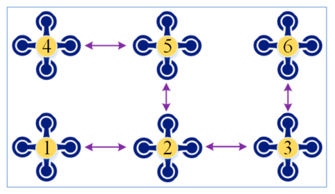
Consider a distributed UAV swarm consisting of six homogeneous UAVs. The interaction topology among the UAVs is shown in Figure 1. If UAV $i$ can receive state information from UAV $j$, then $w_{ij}=1$; otherwise, $w_{ij}=0$. We adopt dynamic model (2) for the swarm, where the system matrix and the input matrix are specified as

$$A=\left[\begin{array}{cc}0& 1\\ 0& 0\end{array}\right]\otimes I_3,B=\left[\begin{array}{c}0\\ 1\end{array}\right]\otimes I_3,$$

where $x_i\left(t\right)={[p_i^{\mathrm{T}}(t),v_i^{\mathrm{T}}\left(t\right)]}^{\mathrm{T}}\in {\mathbb{R}}^6\left(i=1,2,\cdots ,6\right)$.$p_i\left(t\right)={\left[p_i^X\left(t),p_i^Y\right(t),p_i^Z\left(t\right)\right]}^{\mathrm{T}}$ and $v_i\left(t\right)={\left[v_i^X\left(t),v_i^Y\right(t),v_i^Z\left(t\right)\right]}^{\mathrm{T}}$ represent the position and the velocity state variables along the X-, Y-, and Z-axes, respectively. The initial states of all UAVs are set as $x_1\left(0\right)={\left[\begin{array}{cccccc}-2& 4& 5& 3& -2& 5\end{array}\right]}^{\mathrm{T}}$, $x_2\left(0\right)={\left[\begin{array}{cccccc}3& 5& 3& 1& -3& 6\end{array}\right]}^{\mathrm{T}}$, $x_3\left(0\right)={\left[\begin{array}{cccccc}-2& 2& 2& -1& 6& 4\end{array}\right]}^{\mathrm{T}}$, $x_4\left(0\right)={\left[\begin{array}{cccccc}1& 0& 3& 4& 5& 8\end{array}\right]}^{\mathrm{T}}$, $x_5\left(0\right)={\left[\begin{array}{cccccc}-1& -5& 5& 2& -4& -4\end{array}\right]}^{\mathrm{T}}$, $x_6\left(0\right)=\left[\begin{array}{cc}2& 2\end{array}\right.$ ${\left.\begin{array}{cccc}1& -1& 3& 5\end{array}\right]}^{\mathrm{T}}$.

In the simulation scenario, the swarm is configured to maintain a regular hexagonal formation that rotates about the center at 1.5 rad/s, with each UAV stationed 5 m away from the center. Then, the formation vectors of the swarm system are chosen as

$$\begin{array}{ccc}{h}_i\left(t\right)=r[cos\left(1.5t+{\displaystyle \frac{i\pi }{3}}\right)& sin\left(1.5t+{\displaystyle \frac{i\pi }{3}}\right)& -cos\left(1.5t+{\displaystyle \frac{i\pi }{3}}\right)\\ -sin\left(1.5t+{\displaystyle \frac{i\pi }{3}}\right)& cos\left(1.5t+{\displaystyle \frac{i\pi }{3}}\right)& sin\left(1.5t+{\displaystyle \frac{i\pi }{3}}\right){]}^{\mathrm{T}}\end{array},$$

where $i=1,2,\cdots ,6$ and $r=5$. Then, let $\overline{B}B=I_3$ and $\tilde{B}B=0$ with

$$\overline{B}=\left[\begin{array}{cccccc}0& 0& 0& 1& 0& 0\\ 0& 0& 0& 0& 1& 0\\ 0& 0& 0& 0& 0& 1\end{array}\right],\tilde{B}=\left[\begin{array}{cccccc}1& 0& 0& 0& 0& 0\\ 0& 1& 0& 0& 0& 0\\ 0& 0& 1& 0& 0& 0\end{array}\right].$$

5.1. Original Formation Without the Dual-Channel Induced Countermeasure Signals

For the swarm, the gain matrix $K$ that renders the subsystem specified asymptotically stable can be obtained using the linear quadratic regulator method as follows:

$$K=\left[\begin{array}{cccccc}4.3906& 0& 0& 7.3322& 0& 0\\ 0& 4.3906& 0& 0& 7.3322& 0\\ 0& 0& 4.3906& 0& 0& 7.3322\end{array}\right].$$

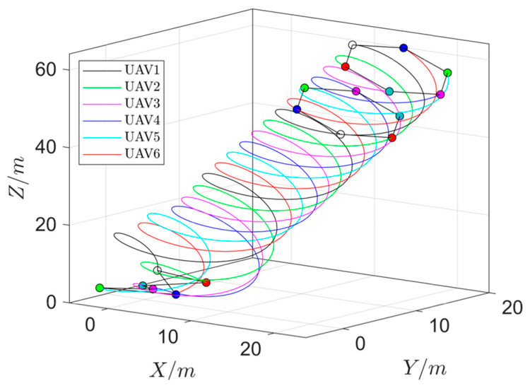
Figure 2 shows the flight trajectories of the distributed UAV swarm in three-dimensional space. We observe that, with the effects of the formation control protocol, the six UAVs within the swarm form a regular hexagon formation and rotate upward around the formation center, with the rotation radius around the circular center being 5 m.

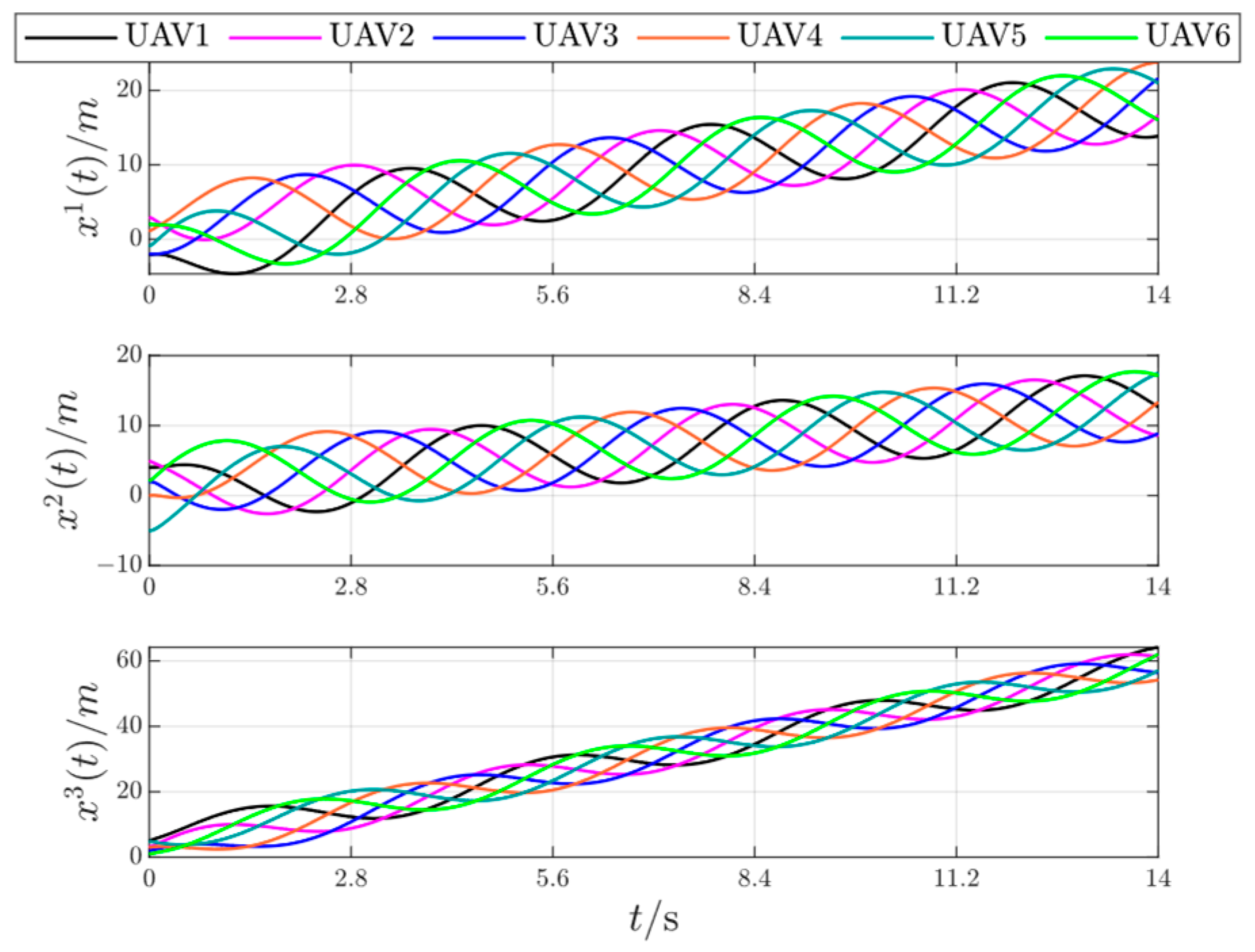
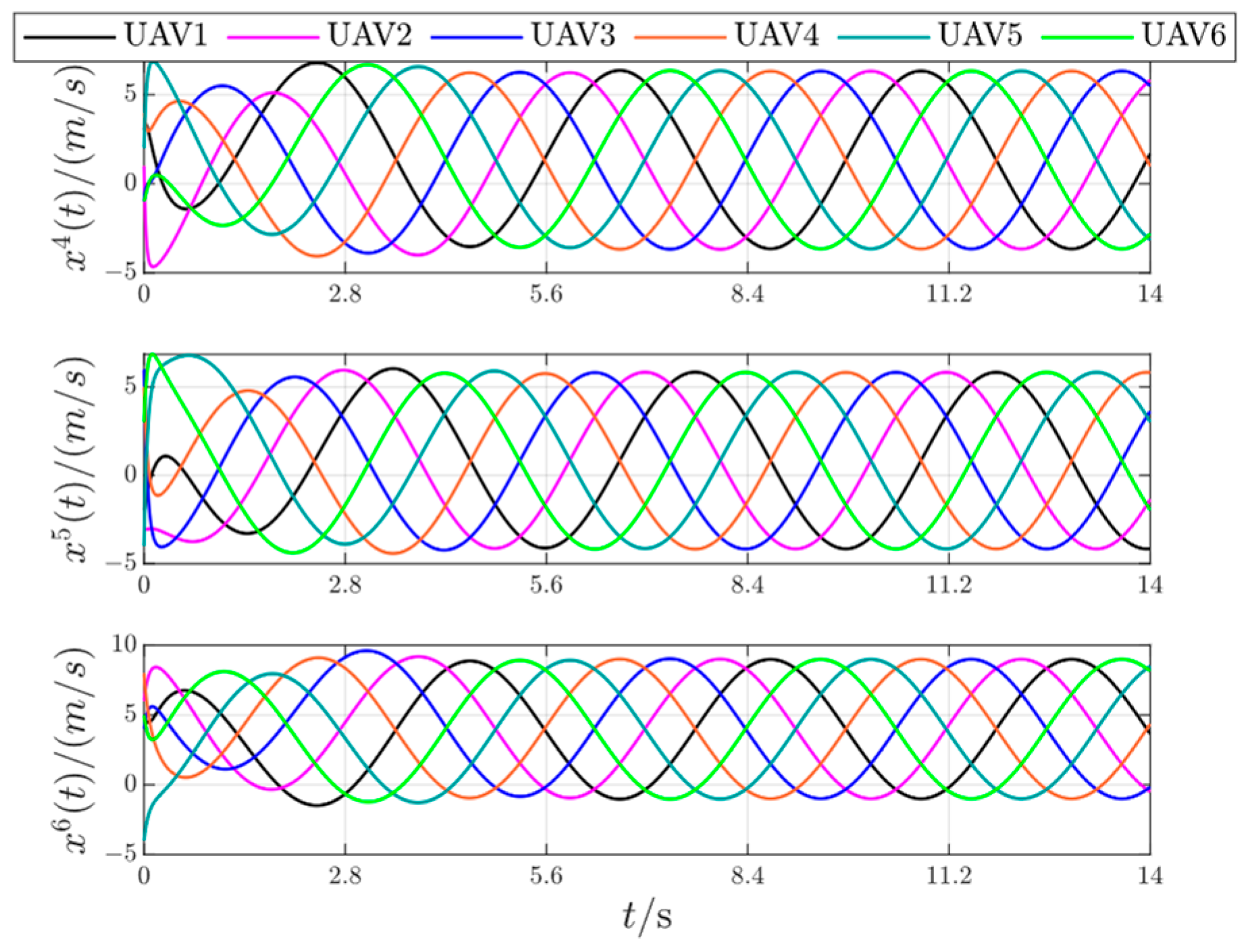
Figure 3 shows the variations in the position states of the six UAVs in the X-, Y-, and Z-axes, and Figure 4 shows the variations in the velocity states. By analyzing the curves in Figure 3 and Figure 4, it can be seen that, at the initial moment, the positions and velocities of the UAVs along the three axes are in a disordered state. After $t=2 s$, the UAVs form the expected formation and maintain the formation structure during the flight.

5.2. Effects of the DCICS for the Distributed UAV Swarm

Based on the above parameters for the swarm formation control, the effectiveness of the DCICS is verified through simulations in the following. Since the induced countermeasure strategy takes effect after the swarm has achieved the formation structure, the injection instant of the dual-channel induced countermeasure signals is set as $t_a=3 s$. Here, a special countermeasure case is considered where it is assumed that the dual-channel induced countermeasure signals are injected into all UAVs in the swarm, that is, the full-countermeasure scenario for the swarm. For simplicity, according to condition (i) of Corollary 1, it is assumed that all sensor-induced countermeasure signals injected into the swarm satisfy $x_i^a\left(t\right)=e^{At}{x}_i^a\left(0\right)$ and the initial countermeasure signals are $x_i^a\left(t_a\right)={\left[\begin{array}{cccccc}0& 4& 0& -2& 0& 5\end{array}\right]}^{\mathrm{T}}\left(i=1,2,\cdots ,6\right)$. Let the initial states of the countermeasure signal be set as $u_1^a\left(t_0\right)={\left[\begin{array}{ccc}10& 4& 1\end{array}\right]}^{\mathrm{T}}$, $u_2^a\left(t_0\right)={\left[\begin{array}{ccc}5& 0& 2\end{array}\right]}^{\mathrm{T}}$, $u_3^a\left(t_0\right)={\left[\begin{array}{ccc}2& -8& 4\end{array}\right]}^{\mathrm{T}}$, $u_4^a\left(t_0\right)={\left[\begin{array}{ccc}-5& -5& 6\end{array}\right]}^{\mathrm{T}}$, $u_5^a\left(t_0\right)=\left[\begin{array}{cc}-8& 5\end{array}\right.$ ${\left.-2\right]}^{\mathrm{T}}$, $u_6^a\left(t_0\right)={\left[\begin{array}{ccc}3& 9& 0\end{array}\right]}^{\mathrm{T}}$.

The relevant countermeasure parameters in Theorem 3 can be set as ${\alpha }_1={\alpha }_2=1$, $F=\mathrm{diag}\left\{0.5,0.5,0.5\right\}$, and the matrix $Y$ can be obtained as follows:

$$Y=\left[\begin{array}{cccccc}2.9031& 0.5994& 0& 0& 0& 0\\ 0.5994& 0.8094& 0& 0& 0& 0\\ 0& 0& 2.9031& 0.5994& 0& 0\\ 0& 0& 0.5994& 0.8094& 0& 0\\ 0& 0& 0& 0& 2.9031& 0.5994\\ 0& 0& 0& 0& 0.5994& 0.8094\end{array}\right].$$

According to Theorem 3, the generation matrix of the actuator-induced countermeasure signal can be obtained as follows:

$$M=\left[\begin{array}{ccc}-0.8094& 0& 0\\ 0& -0.8094& 0\\ 0& 0& -0.8094\end{array}\right].$$

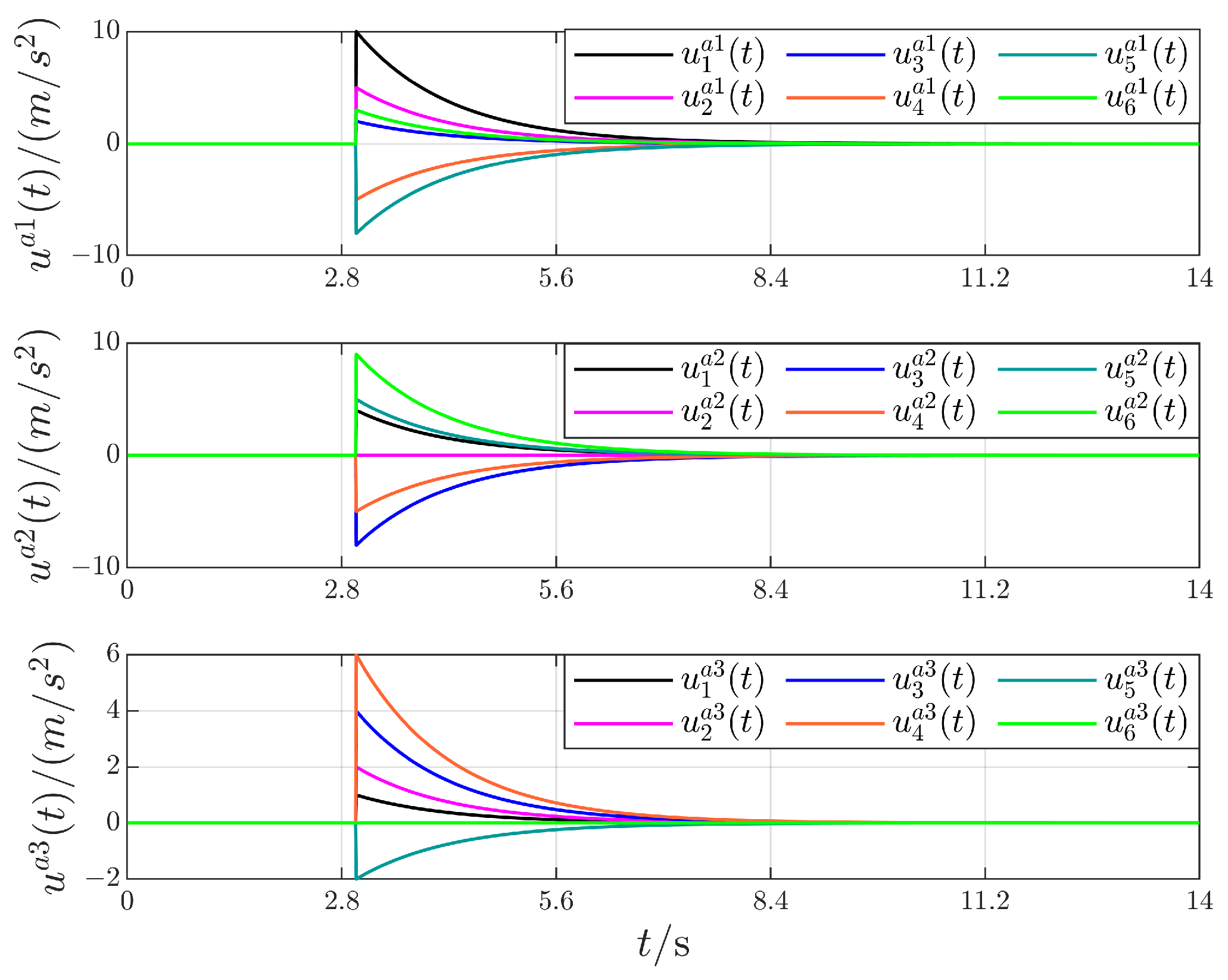
Figure 5 shows the variation curves of the actuator-induced countermeasure signal. It can be seen that under the action of the generation matrix $M$, the actuator-induced countermeasure signal on the three axes eventually achieves asymptotic stability, which conforms to the characteristics of the square integrable signals.

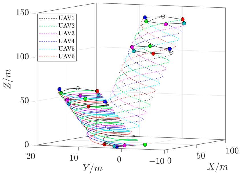
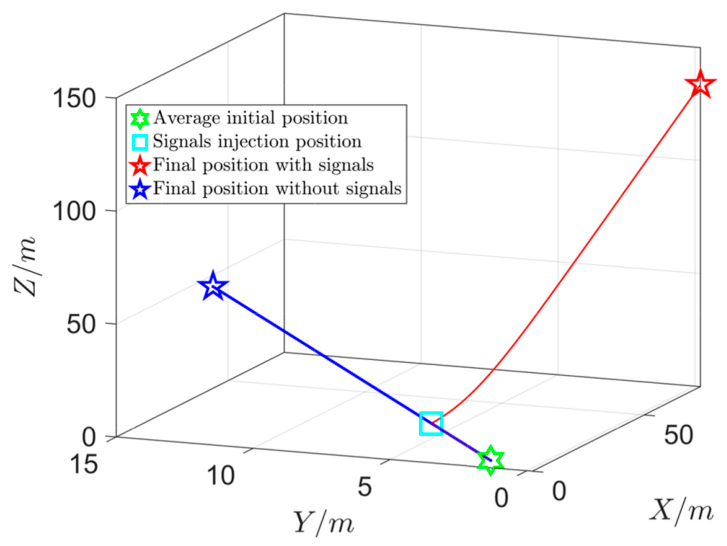
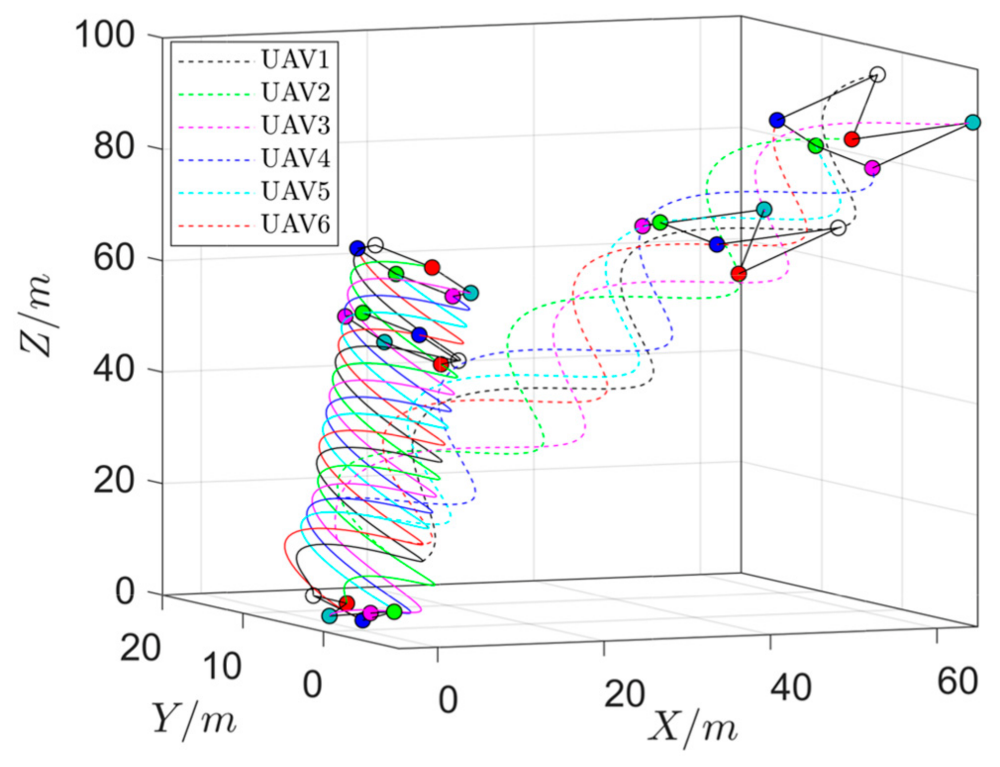
Figure 6 shows a comparison of the swarm flight trajectories before and after the induced countermeasure. The trajectory followed by the formation center is depicted in Figure 7, where the green hexagon indicates the initial formation center position of the swarm; the red and blue pentagrams represent the final formation center positions of the swarm with and without the dual-channel induced countermeasure signals, respectively; and the cyan square indicates the injection position of the DCICS.

From Figure 6 and Figure 7, we observe that the swarm significantly deviates from the original formation flight trajectory under the effects of the dual-channel induced countermeasure signals, and subsequently flies along the prescribed countermeasure flight trajectory. Meanwhile, the UAVs within the swarm maintain the original regular hexagonal formation and perform circular rotation flights with a radius of 5 m around the formation center. As shown in Figure 6, it can be noted that upon the injection of the dual-channel induced countermeasure signals, the formation of the swarm exhibits transient disorder. However, the swarm can recover and maintain the original formation structure quickly, thereby realising the expected countermeasure effect. In the absence of the countermeasure signals, the final positions of the six UAVs are (13.84, 12.64, 64.15) m, (16.64, 8.50, 61.35) m, (21.63, 8.85, 56.36) m, (23.82, 13.35, 54.17) m, (21.01, 17.49, 56.98) m, and (16.03, 17.14, 61.96) m, respectively. Under the action of the dual-channel induced countermeasure signals, the final positions are driven to (71.98, 0.69, 141.34) m, (74.77, −3.45, 138.54) m, (79.76, −3.09, 133.55) m, (81.94, 1.39, 131.37) m, (79.14, 5.54, 134.17) m, and (74.16, 5.18, 139.15) m. As shown in Figure 7, the formation center of the swarm is induced to shift from (18.83, 13.00, 59.16) m to (76.96, 1.04, 136.35) m, yielding a total displacement of 97.36 m. These results confirm a significant countermeasure effect.

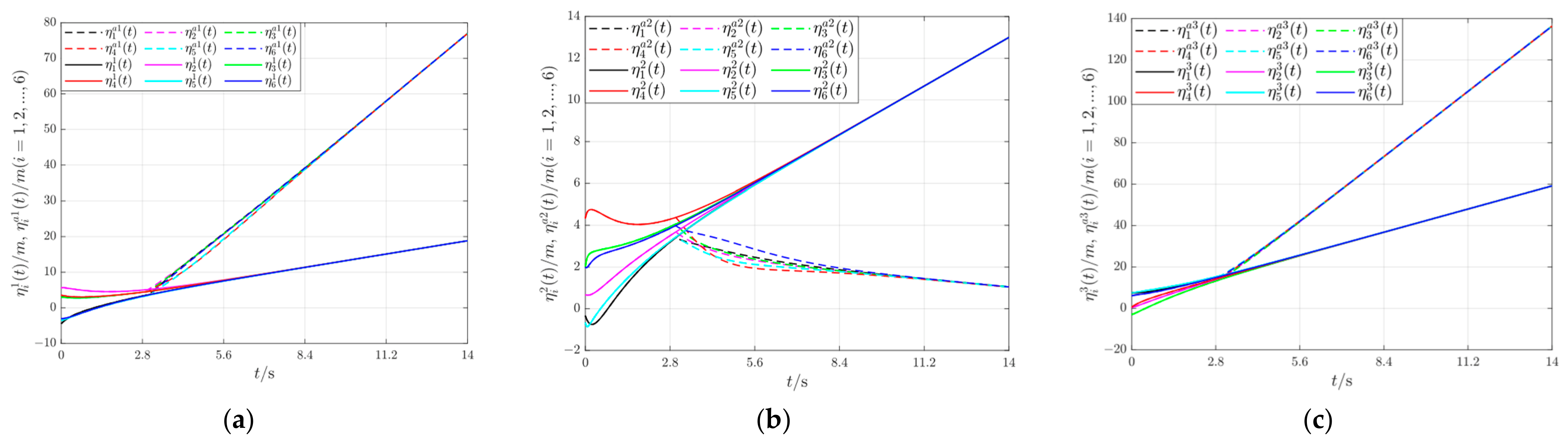
Let ${\eta }_i^k\left(t\right)=x_i^k\left(t\right)-h_i^k\left(t\right)\left(i,k=1,2,\cdots ,6\right)$ denote the difference between the position or velocity state of UAV $i$ in the absence of the countermeasure signals and the formation error. Likewise, let ${\eta }_i^{ak}\left(t\right)=x_i^{ak}\left(t\right)-h_i^k\left(t\right)\left(i,k=1,2,\cdots ,6\right)$ denote the formation error of the position or velocity of UAV $i$ when subjected to the proposed countermeasure strategy.

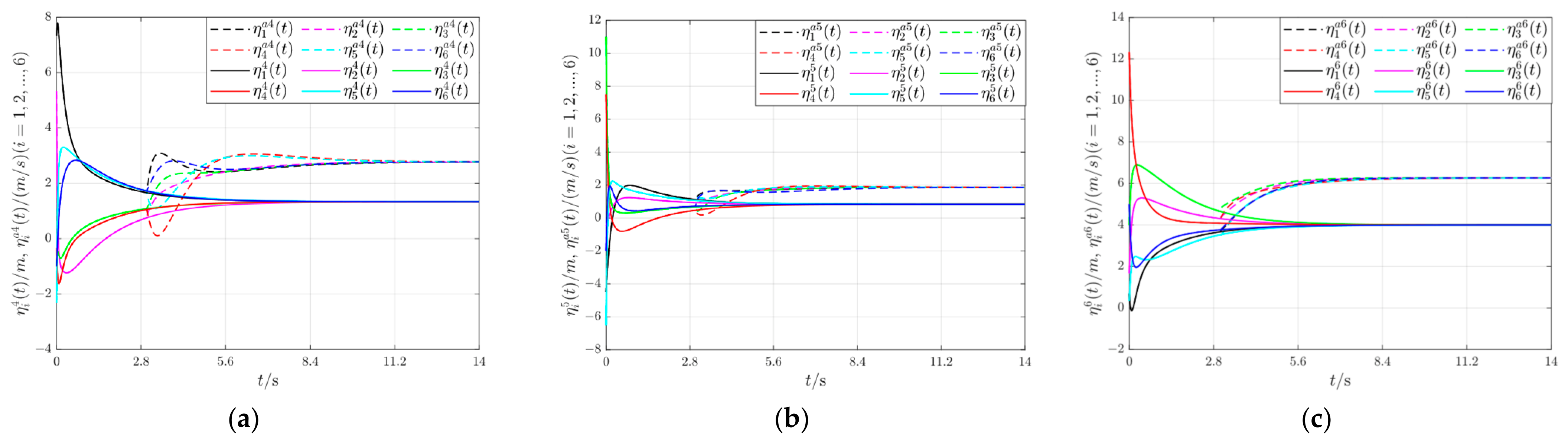
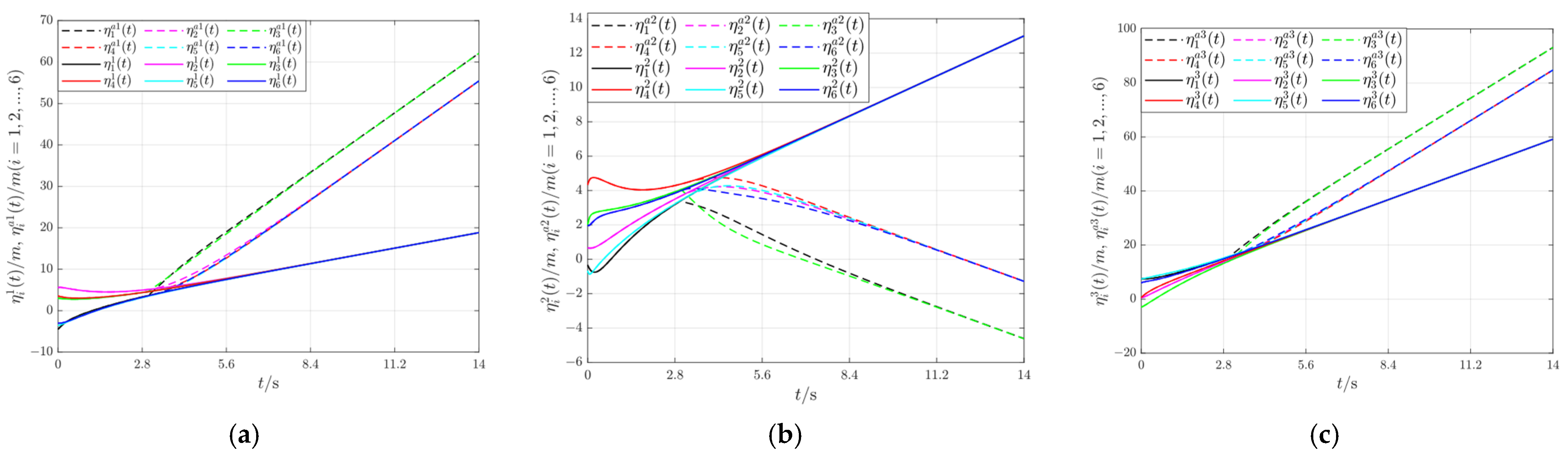
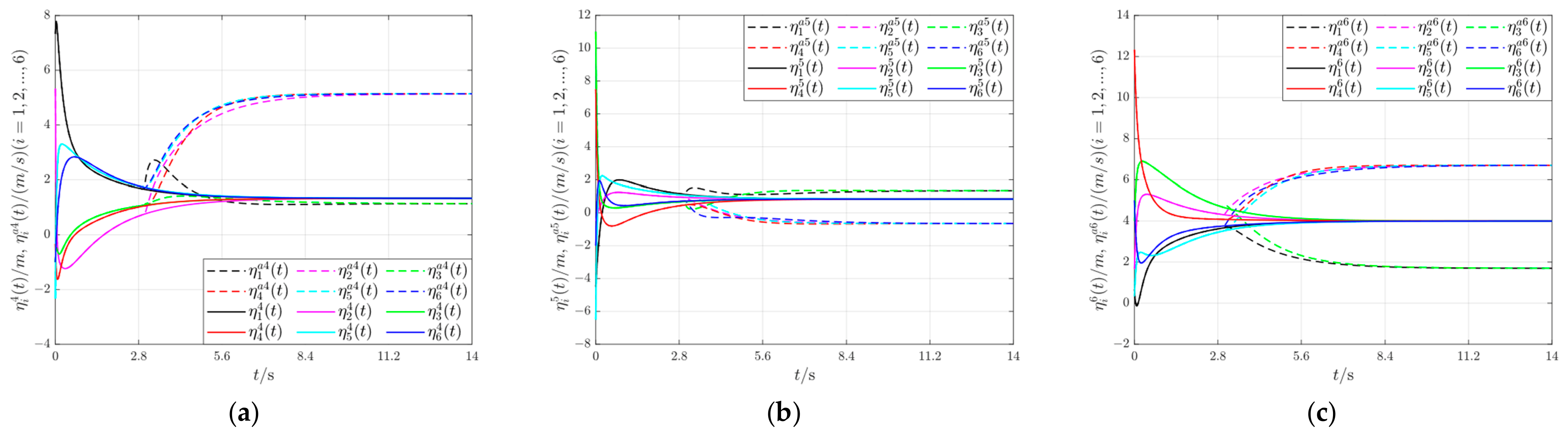
Figure 8 and Figure 9 show the formation errors of the swarm with and without the dual-channel induced countermeasure signals along the X-, Y-, and Z-axes. From the analysis of Figure 8 and Figure 9, it can be seen that in the absence of the dual-channel induced countermeasure signals, both the position and the velocity formation errors converge to consensus, indicating that the swarm achieves the expected formation successfully. Specifically, the position formation errors along the X-, Y-, and Z-axes reach 18.8 m, 12.97 m, and 58.88 m, respectively, while the velocity formation errors along the three axes converge to 1.33 m/s, 0.83 m/s, and 3.99 m/s, respectively. After the injection of the dual-channel induced countermeasure signals, the position and velocity formation errors exhibit a temporary disorder and gradually converge to consensus, but there is a deviation from the original formation error. The position formation errors ultimately settle at 76.62 m, 1.05 m, and 135.34 m along the X-, Y-, and Z-axes, respectively, corresponding to deviations of 57.82 m, −11.92 m, and 76.46 m. Likewise, the velocity formation errors along the three axes converge to 2.77 m/s, 1.86 m/s, and 6.26 m/s, respectively, with deviations of 1.44 m/s, 1.03 m/s, and 2.77 m/s. The results demonstrate that the swarm maintains the formation structure while the position states and the velocity states are altered, and the countermeasure flight trajectory is different from the original formation flight trajectory. Based on Figure 6, Figure 7, Figure 8 and Figure 9, it can be concluded that the induced countermeasure against the swarm can be realised by the DCICS.

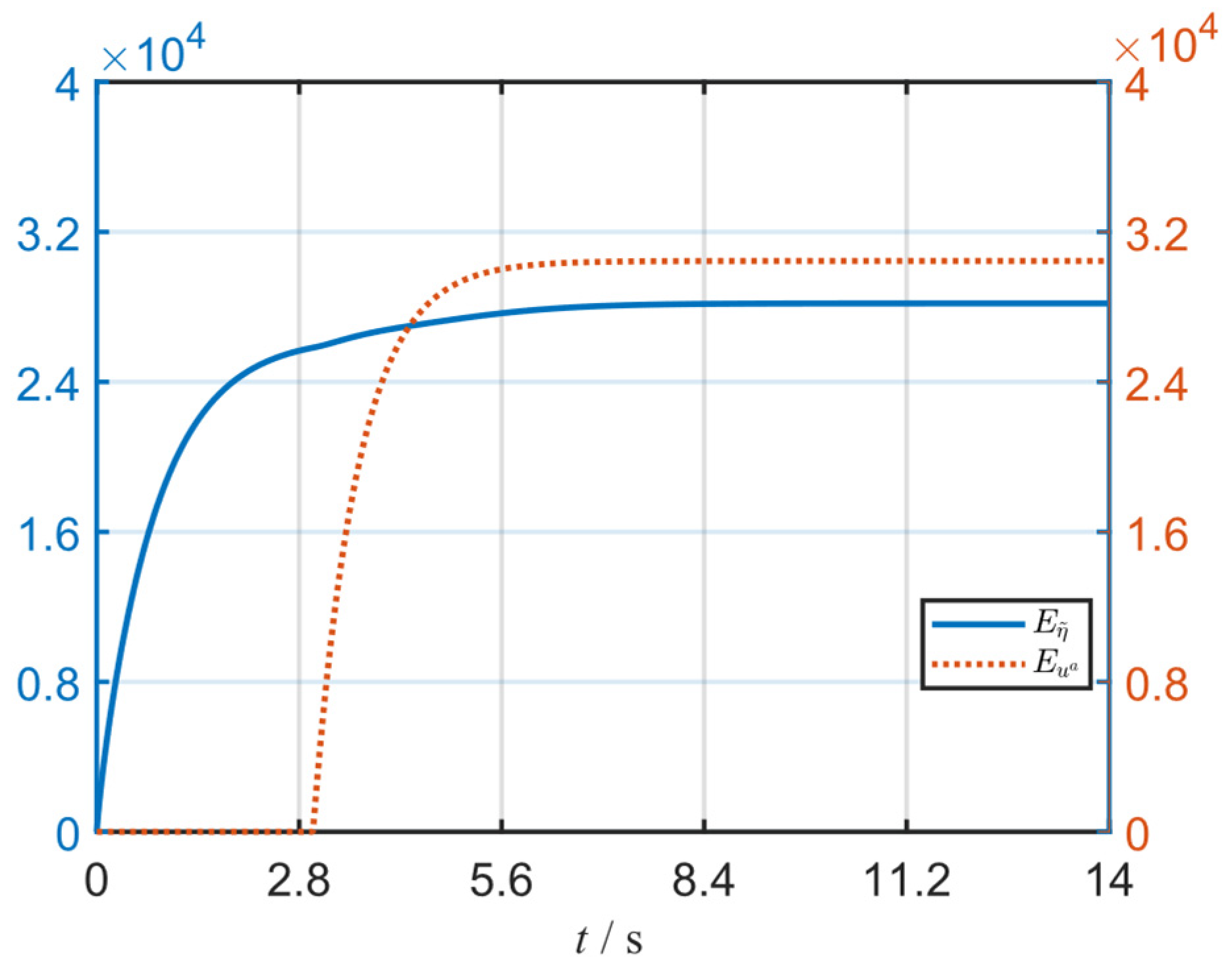
Let $E_{\tilde{\eta }}$ and $E_{u^a}$ denote the energies of the formation error and the actuator-induced countermeasure signal, respectively. A lower formation error energy implies a milder disturbance to the formation structure caused by the dual-channel induced countermeasure signals, whereas a higher actuator-induced countermeasure signal energy results in greater disruption to the formation structure. It should be noted that within the robust $H_{\infty }$ performance framework, the performance factors ${\alpha }_1$ and ${\alpha }_2$ determine the relative weighting between the formation error energy and the allowable energy of the actuator-induced countermeasure signal. A smaller relative weight ${\displaystyle {\alpha }_2/{\alpha }_1}$ leads to a more conservative design of the actuator-induced countermeasure signal, constraining the formation error energy to a lower level but simultaneously reducing the feasible set of the LMIs in the design criterion for the actuator-induced countermeasure signal. Conversely, a larger relative weight ${\displaystyle {\alpha }_2/{\alpha }_1}$ expands the feasible set of the LMIs at the cost of imposing a stronger impact on the formation structure. In the simulations, the selected parameter values are intended to guarantee LMI feasibility while preserving a significant induced effect and maintaining acceptable transient formation errors. These values are not globally optimal, but rather provide a feasible design point for illustrating the proposed robust $H_{\infty }$ performance framework.

Figure 10 shows the energy variation curve of $E_{\overline{\eta }}$ and $E_{u^a}$. It can be seen that the effect of the dual-channel induced countermeasure signals causes fluctuations in the formation error. After the injection of the countermeasure signals, the energy of the actuator-induced countermeasure signal surpasses that of the formation error at $t=4.26 \mathrm{s}$. After the swarm reaches a steady state, the formation error energy stabilizes at 28,187.9, while the actuator-induced countermeasure signal energy stabilizes at 30,452.2. The accumulated energy of the formation errors is less than the energy of the actuator-induced countermeasure signal, which is consistent with the theoretical result. Furthermore, the ratio of the formation error energy to the actuator-induced countermeasure signal energy is approximately $E_{\overline{\eta }}/E_{u^a}\approx 0.925$, which is below the theoretical upper bound ${\displaystyle {\alpha }_2/{\alpha }_1}=1$. This confirms that the robust $H_{\infty }$ performance constraint is satisfied.

To validate the scalability and robustness of the DCICS when partial UAVs receive the induced countermeasure signals, we consider a more general case, that is, the partial-countermeasure scenario for the swarm. Specifically, the dual-channel induced countermeasure signals are injected into only UAV 1 and UAV 3, while all other simulation parameters are kept identical to those in the full-countermeasure scenario for the swarm.

Figure 11 compares the flight trajectories of the swarm with and without the countermeasure signals under the partial-countermeasure scenario. As shown in Figure 11, the overall flight trajectory of the swarm exhibits a significant deviation after the countermeasure signals are applied. Specifically, the final positions of UAV 1 and UAV 3, which are directly injected with the countermeasure signals, shift from (13.84, 12.64, 64.15) m and (21.63, 8.85, 56.36) m to (57.13, −4.96, 98.13) m and (64.91, −8.76, 90.34) m, respectively, while the final positions of the remaining UAVs also change accordingly. These results confirm that the expected countermeasure effect has been achieved when the countermeasure signals are injected into partial UAVs, and demonstrate the robustness of the DCICS.

It should be noted that, according to Definition 1, with the dual-channel induced countermeasure signals, the swarm formation is formed by the sum of the true states of all UAVs and the sensor-induced countermeasure signals injected into each UAV, and the swarm moves collectively along the countermeasure flight trajectory. However, in the partial-countermeasure scenario, since the sensor-induced countermeasure signals are injected into only partial UAVs, the true states of the injected and uninjected UAVs cannot fully form the original formation structure. As is also evident from Figure 11, the flight trajectories of the injected UAVs deviate from the overall countermeasure flight trajectory of the swarm, and this deviation corresponds precisely to the sensor-induced countermeasure signals. Therefore, although the original formation structure cannot be perfectly realised, the flight trajectories of all UAVs remain controllable, and the DCICS can still achieve the expected countermeasure effect under the partial-countermeasure scenario.

Figure 12 and Figure 13 present the position and velocity formation errors along the X-, Y-, and Z-axes before and after the induced countermeasure. From Figure 12, it can be observed that in the absence of countermeasure signals, the position formation errors of the swarm converge to consensus, indicating that the swarm achieves the expected formation. After the countermeasure signals are injected, the position formation errors of the injected UAVs change first, followed by those of the remaining UAVs. Eventually, the position formation errors of UAV 1 and UAV 3 converge to one consensus value, while those of the other UAVs converge to another. At steady state, the deviations between these two groups are −6.56 m in the X-axis, 3.3 m in the Y-axis, and −8.01 m in the Z-axis. Figure 13 shows that, in the absence of the countermeasure signals, the velocity formation errors of all UAVs converge to consensus. After the injection of the countermeasure signals, the velocity formation errors of UAV 1 and UAV 3 converge to 1.14 m/s, 1.34 m/s, and 1.7 m/s along the X-, Y-, and Z-axes, respectively, while those of the remaining UAVs converge to 5.14 m/s, −0.65 m/s, and 6.69 m/s, respectively. The resulting deviations between the two groups are 4 m/s in the X-axis, −1.99 m/s in the Y-axis, and 4.99 m/s in the Z-axis, which exactly match the values of the sensor-induced countermeasure signal. These results confirm the consistency between the simulations and the theoretical analysis.

5.3. Simulations for Comparative Verification

This section presents comparative simulations to validate the proposed DCICS. First, a comparison with single-channel induced countermeasure strategies is conducted, where countermeasure signals are injected exclusively into either the SC channel or the CA channel. Subsequently, Monte Carlo simulations are conducted to verify the robustness of the proposed strategy under random perturbations.

5.3.1. Single-Channel Induced Countermeasure Simulations

In the single-channel induced countermeasure simulations, the countermeasure signals are injected exclusively into either the SC channel or the CA channel, while all other parameters remain identical to those employed in the full countermeasure scenario of the dual-channel induced countermeasure simulations.

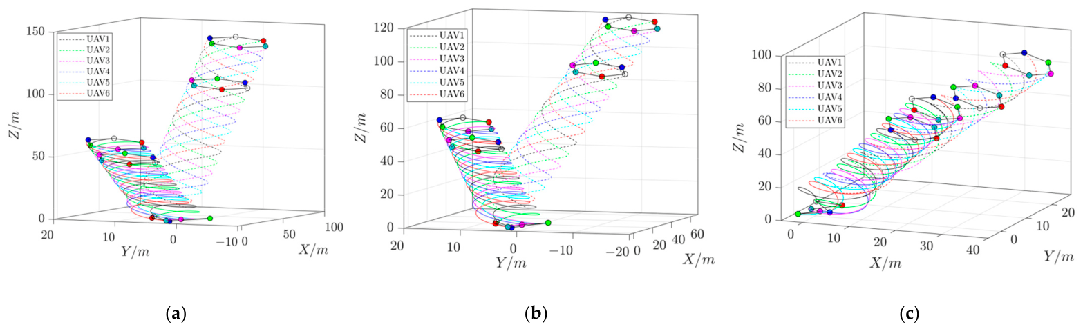
Figure 14 compares the trajectory deviations of the swarm under three different induced countermeasure strategies. Specifically, Figure 14a, Figure 14b, and Figure 14c present the warm trajectory comparisons for the dual-channel, the SC channel, and the CA induced countermeasure strategies, respectively. The comparative results indicate that all three strategies are capable of deviating the swarm flight trajectories. Under the DCICS, the overall trajectory of the swarm exhibits a significant deviation, demonstrating that coordinated injection through both the SC and CA channels produces a superposition effect that enhances countermeasure effectiveness. When the countermeasure signals are injected only into the SC channel, the trajectory deviation is constrained by the feedback gain and communication topology of the formation control protocol, since the sensor-induced countermeasure signals must propagate through the distributed interaction network of the swarm. In the actuator-induced countermeasure strategy, the countermeasure signals act directly on the control inputs of the UAVs. However, as the actuator-induced countermeasure signals are energy-bounded, the degree of trajectory deviation is limited, and the countermeasure flight trajectories offer restricted design flexibility.

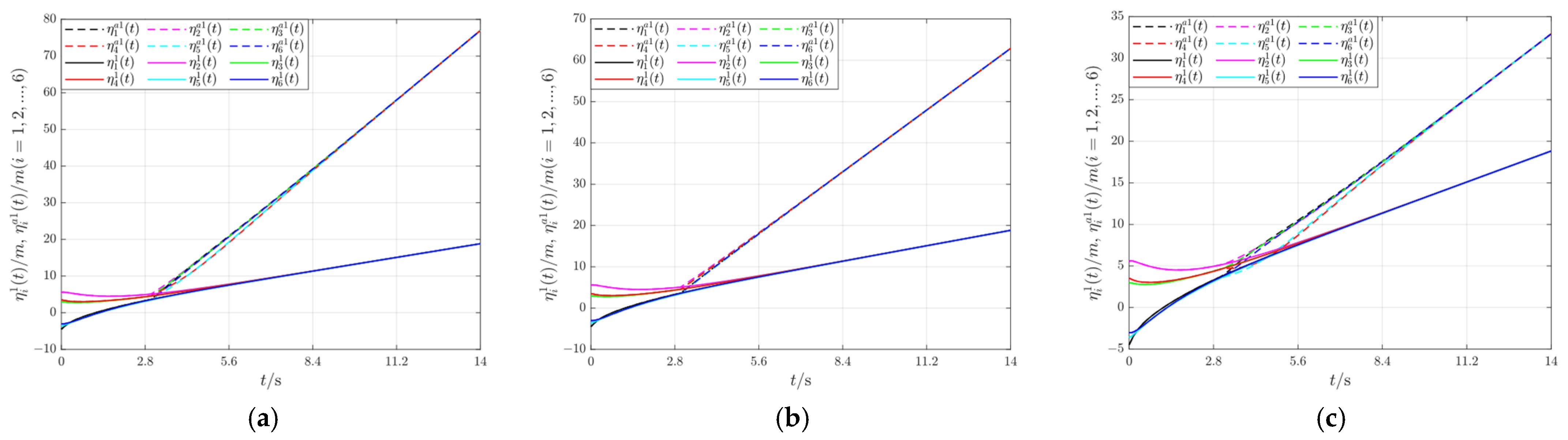
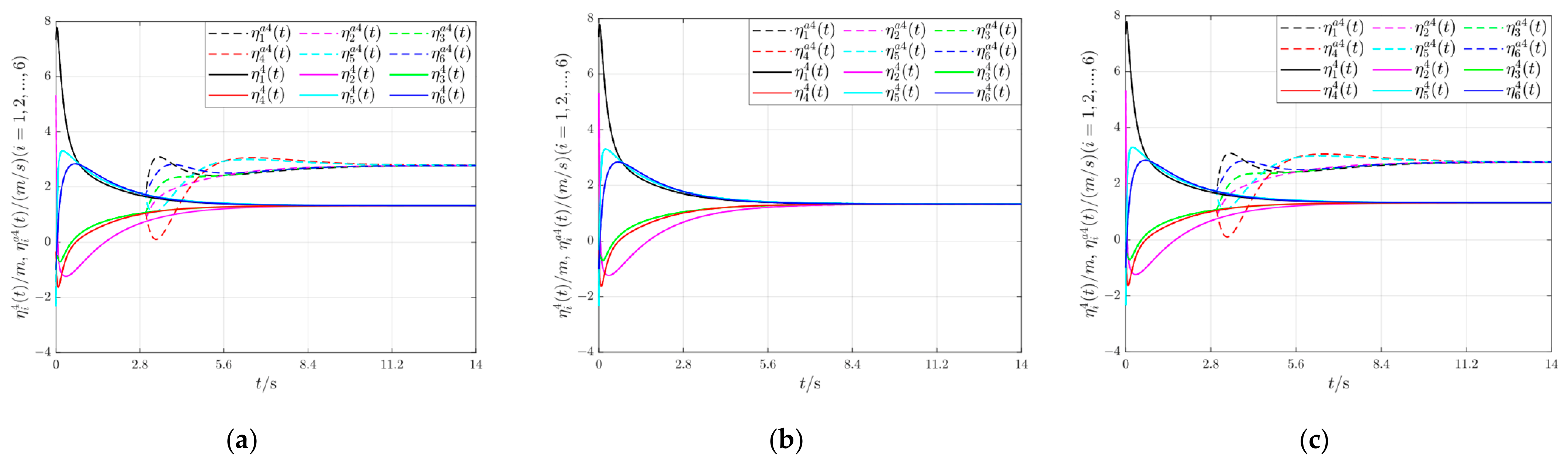
We compare the position and velocity of the swarm under different countermeasure strategies, taking the X-axis as a representative example. Figure 15 and Figure 16 present the position and velocity profiles along the X-axis under the three induced countermeasure strategies, respectively. From Figure 15, it can be observed that in the absence of the countermeasure signals, the swarm position along the X-axis ultimately reaches 18.8 m. Under the DCICS, the X-axis positions of the swarm converge after 8.33 s and finally reach 76.62 m along the X-axis, representing a deviation of 57.82 m from the nominal case. For the sensor-induced countermeasure strategy, the X-axis positions of the swarm converge after 5.14 s and ultimately reach 62.87 m along the X-axis, with a deviation of 44.07 m. For the actuator-induced countermeasure strategy, the X-axis positions of the swarm converge after 10.28 s and finally reach 14.12 m along the X-axis, deviating by 32.92 m. These results indicate that the sensor-induced countermeasure strategy causes relatively minor disruption to the swarm, whereas the actuator-induced countermeasure strategy inflicts greater damage and necessitates a longer recovery time.

From Figure 16, it can be observed that in the absence of the countermeasure signals, the swarm velocity along the X-axis stabilizes at 1.33 m/s, whereas under the DCICS, it ultimately converges to 2.77 m/s. Notably, under the sensor-induced countermeasure strategy, the actual velocities of the swarm remain unchanged from the nominal case. This is because the sensor-induced countermeasure signals are injected into the SC channel and influence the generation of control commands without directly altering the actual velocity states of the UAVs. In contrast, the actuator-induced countermeasure signals act directly on the control inputs and therefore modify the actual velocity responses. The X-axis velocity of the swarm under the actuator-induced countermeasure strategy converges to the same value as under the DCICS, which reflects the superimposed effect arising from the coordination of the sensor-induced and actuator-induced countermeasure signals.

It should be noted that, as illustrated in Figure 14, Figure 15 and Figure 16, both the sensor-induced and actuator-induced countermeasure strategies are capable of inducing swarm trajectory deviations. However, the DCICS exhibits superior formation cooperative performance, as evidenced by smoother and more consistent trajectories across individual UAVs. Under single-channel induced countermeasure strategies, the absence of one control channel renders the swarm trajectory response sluggish and incoherent. Therefore, the practical advantage of the DCICS does not lie in outperforming single-channel strategies on any single metric, but rather in providing a more balanced and flexible design framework that integrates the complementary strengths of both channels, thereby offering enhanced practicality and scalability for actual deployment.

5.3.2. Monte Carlo Simulations

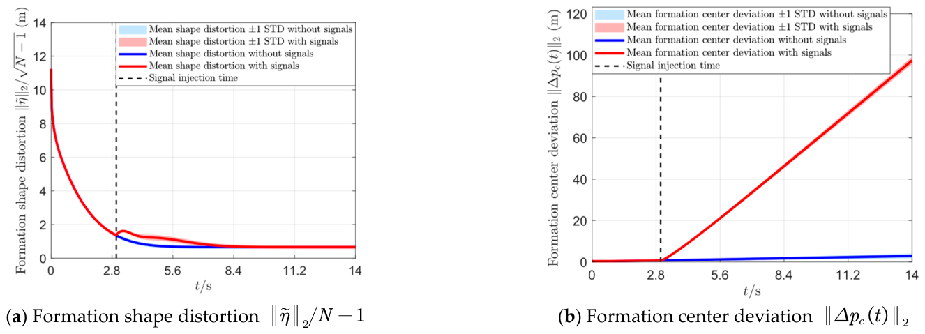
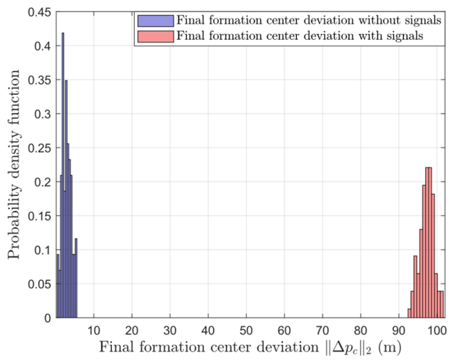
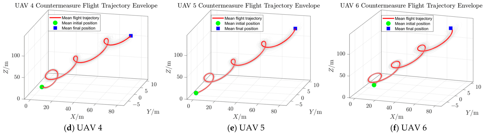
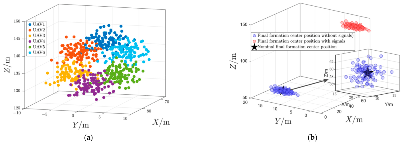
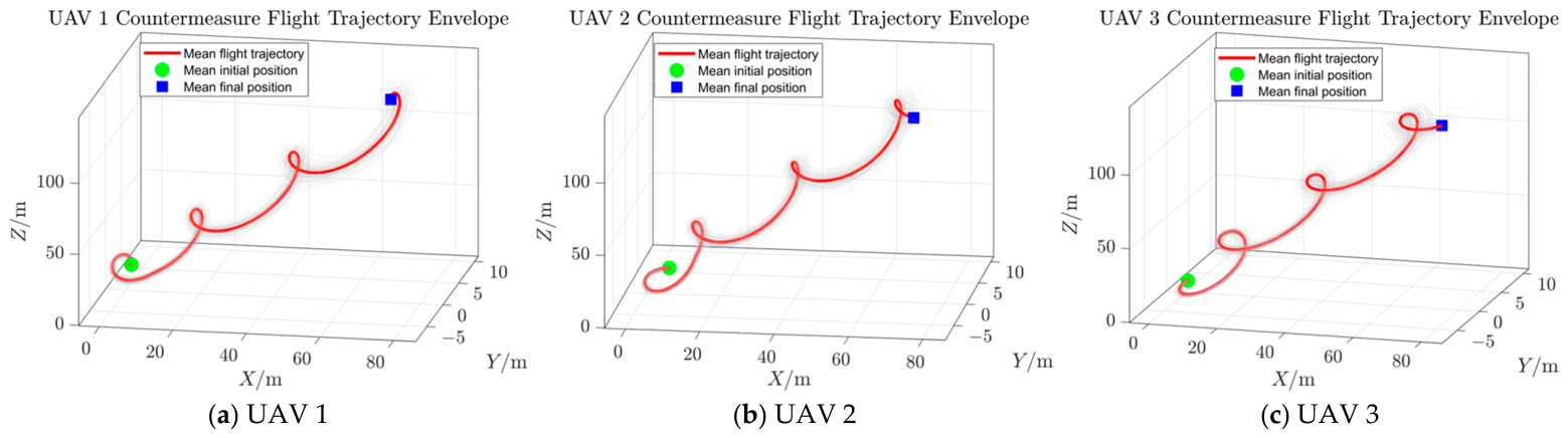
To evaluate the robustness of the proposed DCICS under non-ideal conditions, we conduct Monte Carlo comparative simulations by introducing random initial state perturbations, localization errors, measurement noise, and communication delays. Specifically, the standard deviations of random initial position perturbations, random initial velocity perturbations, and localization errors are set to 0.5 m, 0.3 m/s, and 0.2 m, respectively, while the communication delay is set to 3 s. All other simulation parameters remain consistent with those in the full-countermeasure scenario of the dual-channel induced countermeasure simulations. If the formation center deviation distance of the swarm after countermeasure exceeds 20 m, it is determined that the overall flight trajectory of the swarm has deviated significantly from the original formation flight trajectory, indicating a pronounced countermeasure effect.

Figure 17 presents the evolution of the formation shape distortion ${\displaystyle \Vert \tilde{\eta }{\Vert }_2/N-1}$ and formation center deviation $\Vert \Delta p_c\left(t\right){\Vert }_2$ over time in the Monte Carlo simulations. In Figure 17a, we observe that in the absence of the countermeasure signals, the mean formation shape distortion rapidly converges from an initial value of 11.25 m to 0.66 m, indicating that the swarm successfully forms and maintains the desired formation structure from an initially disordered state. After the countermeasure signal is injected, the mean formation shape distortion exhibits a transient increase with a peak value of 1.61 m, after which it gradually declines and stabilizes to the same level as that without countermeasure signals. This behavior indicates that, although the DCICS temporarily disrupts the formation structure, the swarm can recover the original formation structure within a certain period of time. The narrow shaded regions in both cases, tightly concentrated around the mean curves, further indicate that moderate stochastic disturbances do not compromise the formation maintenance performance.

In Figure 17b, we observe that without the countermeasure signals, the formation center deviation remains below 3 m throughout the simulations, with a peak value of 2.85 m, confirming that the formation center stays close to the nominal position despite random perturbations. In contrast, once the countermeasure signal is injected, the formation center deviation exhibits a significant and approximately linear growth, reaching 97.33 m at $t=14 \mathrm{s}$. The significant gap between the two curves quantitatively validates the effectiveness of the DCICS in driving the formation center away from its nominal position. Moreover, at $t=14 \mathrm{s}$, the mean $\pm 1$ standard deviation of the formation center deviation under the countermeasure signals falls within the interval [95.44, 99.04] m, further confirming consistent and robust induced eviction effects in the presence of stochastic uncertainties. Notably, the formation maintenance and the formation center deviation occur concurrently. The results reveal that the swarm undergoes significant positional eviction while maintaining the original formation structure, which is consistent with the theory.

Figure 18a presents the three-dimensional scatter distribution of the final positions of the swarm with the dual-channel induced countermeasure signal across all Monte Carlo simulations. Despite the presence of stochastic disturbances throughout the simulations, the position clouds of each UAV exhibit clear clustering behavior, and the relative spatial relationships among the six UAVs conform to the prescribed formation. The overlap between adjacent clusters is limited, and the overall spatial arrangement exhibits a coordinated and consistent formation structure rather than random dispersion. The visual results indicate that the UAVs maintain their original geometric constraints during the countermeasure process, thereby preserving the structural integrity of the formation at the individual level. Figure 18b compares the final formation center positions of the swarm with and without the countermeasure signals in three-dimensional space under stochastic disturbances. The red and blue circles represent the final formation center positions with and without the countermeasure signal, respectively, while the black pentagram denotes the nominal final formation center position of the swarm without the countermeasure signals in the absence of random perturbations. As shown in the figure, the final centroids in the absence of the countermeasure signal form a tight cluster around the nominal position, exhibiting a confined spatial spread as detailed in the magnified inset. In contrast, when the countermeasure signals are present, the final centroids significantly deviate from the nominal position. The two clusters are distinctly separated with negligible overlap, which confirms that the consistent and significant displacement of the formation center is induced by the countermeasure strategy under stochastic disturbances.

Figure 19 presents the probability density function of the final formation center deviation $\Vert \Delta p_c{\Vert }_2$ in the Monte Carlo simulations. We observe that in the absence of countermeasure signals, the distribution of the final formation center deviation is concentrated within [0, 5.13] m, with the peak occurring in the interval [1.69, 2.12] m at a probability density of 0.418. In contrast, after the injection of the countermeasure signals, the distribution shifts dramatically toward the interval [92.4, 101.64] m, peaking in the interval [97.02, 98.56] m with a probability density of 0.220. The two distributions exhibit a clear bimodal separation, indicating that the induced countermeasure of the swarm trajectory is statistically significant and highly reproducible across multiple trials. These results quantitatively demonstrate that the DCICS reliably achieves overall trajectory countermeasure of the swarm while maintaining the original formation structure.

Figure 20 illustrates the flight trajectory envelopes of the six UAVs during the induced countermeasure process. We observe that each UAV with the dual-channel countermeasure signals executes a smooth, spiraling ascent trajectory, continuously satisfying the formation constraints imposed by the neighboring UAVs. The thin gray curves are concentrated around the mean countermeasure flight trajectories with limited divergence, indicating that although stochastic disturbances exert minor variations on the swarm trajectories, they do not alter the ultimate countermeasure effect. This behavior demonstrates the robustness of the proposed DCICS against stochastic perturbations.

6. Conclusions

This paper proposes a DCICS with prescribed countermeasure flight trajectories for the formation control of the distributed UAV swarm from the defensive perspective, contributing to the establishment of a safe and resilient civilian low-altitude ecosystem. In this case, the entire swarm can be directionally evicted from the formation flight trajectory to the countermeasure flight trajectory while maintaining formation stability. We establish mathematical models of the sensor-induced countermeasure signal and the actuator-induced countermeasure signal based on practical signal injection means, and corresponding design criteria were provided. By projecting the swarm system into the macro formation element, we give the explicit closed-form expression of the countermeasure flight trajectory, which characterizes the effect of the dual-channel induced countermeasure signals on the flight trajectory of the formation center. Numerical simulation results demonstrate that, in the full-countermeasure scenario, the formation center ultimately deviates from the predetermined position by 97.36 m, while the formation error remains bounded and reconverges after 11.63 s. The ratio of the actuator-induced countermeasure signal energy to the formation error energy is 0.925, which lies within the robust $H_{\infty }$ performance bound α₂/α₁ = 1. In the partial-countermeasure scenario, the formation center ultimately deviates from the predetermined position by 50.27 m, and the expected induced countermeasure effect is still achieved. Comparative simulations against single-channel induced countermeasure strategies and Monte Carlo analysis further validate the performance of the proposed strategy. The proposed DCICS can be applied to safeguard civilian infrastructure, ensure low-altitude public safety, and manage civilian airspace. We will focus future research on the following two aspects. The first is the stealthy induced countermeasure problem for the distributed UAV swarm with advanced attack detection and defense mechanisms. The second is to extend the proof-of-concept to more realistic swarm models and validate the proposed algorithm through countermeasure experiments or hardware-in-the-loop simulations, thereby bridging the gap between theoretical research and practical deployment.

References

1. Du, Z.P.; Luo, C.B.; Min, G.Y.; Wu, J.; Luo, C.; Pu, J.; Li, S. A Survey on Autonomous and Intelligent Swarms of Uncrewed Aerial Vehicles (UAVs). IEEE Trans. Intell. Transp. Syst. 2025, 26, 14477–14500. [Google Scholar] [CrossRef] [Scilit]
2. Guo, Z.Y.; Cao, J.; Ren, X.P.; Zhou, Y.C.; Cheng, L.; Yin, P.J.; Li, H. LDST-UAVS: A Lightweight Data Secure Transmission Protocol for Unmanned Aerial Vehicle Swarms in Emergency Rescue Scenarios. IEEE Trans. Netw. Serv. Manag. 2026, 23, 2258–2279. [Google Scholar] [CrossRef] [Scilit]
3. Guebsi, R.; Mami, S.; Chokmani, K. Drones in Precision Agriculture: A Comprehensive Review of Applications, Technologies, and Challenges. Drones 2024, 8, 686. [Google Scholar] [CrossRef] [Scilit]
4. Zhang, J.; Campbell, J.F.; Sweeney, D.C., II; Hupman, A.C. Energy Consumption Models for Delivery Drones: A Comparison and Assessment. Transp. Res. Part D Transp. Environ. 2021, 90, 102668. [Google Scholar] [CrossRef] [Scilit]
5. Kierzkowski, A.; Dziewoński, B.; Kaliszuk, K.; Kucharski, M. Evaluation of Light Electric Flying-Wing Unmanned Aerial System Energy Consumption during Holding Maneuver. Energies 2025, 18, 1300. [Google Scholar] [CrossRef] [Scilit]
6. Karpiński, P.; Czyż, Z.; Skiba, K.; Parafiniuk, S. Performance Analysis of the Unmanned Aerial Vehicle Based on the Flight Test. In Proceedings of the 2024 11th International Workshop on Metrology for AeroSpace (MetroAeroSpace); IEEE: Lublin, Poland, 2024; pp. 394–398. [Google Scholar]
7. Vashisth, A.; Singh, B.; Batth, R.S. UAV Path Planning: Challenges, Strategies, and Future Directions. In Advances in Mechatronics and Mechanical Engineering; Khalid, S., Siddiqui, N.N., Eds.; IGI Global: Hershey, PA, USA, 2024; pp. 150–174. [Google Scholar]
8. Wei, X.M.; Li, X.H.; Sun, C.; Ma, J.F. Physical Attacks on a UAV System: Overview and Emerging Methods. IEEE Trans. Intell. Transp. Syst. 2025, 27, 2839–2857. [Google Scholar] [CrossRef] [Scilit]
9. Zhang, T.; Lu, R.T.; Yang, X.G.; Xie, X.L.; Fan, J.W.; Tang, B. UAV Hunter: A Net-Capturing UAV System with Improved Detection and Tracking Methods for Anti-UAV Defense. Drones 2024, 8, 573. [Google Scholar] [CrossRef] [Scilit]
10. Geng, X.S.; Guo, Y.; Tang, K.H.; Wu, W.Q.; Ren, Y.C.; Duan, G.D. A Covert Spoofing Algorithm for SINS/GNSS Tightly Integrated Navigation System. IEEE Trans. Autom. Sci. Eng. 2025, 22, 6134–6142. [Google Scholar] [CrossRef] [Scilit]
11. Sherman, M.; Shao, S.H.; Sun, X.; Zheng, J. Counter UAV Swarms: Challenges, Considerations, and Future Directions in UAV Warfare. IEEE Wirel. Commun. 2025, 32, 190–196. [Google Scholar] [CrossRef] [Scilit]
12. Xing, L.; Cui, C.; Wang, M.; Xu, C. From Detection to Countermeasure: A Review of Key Technologies in Counter-Unmanned Aerial Vehicle Systems. IET Cyber-Syst. Robot. 2026, 8, e70048. [Google Scholar] [CrossRef] [Scilit]
13. Xing, H.J.; Xu, Y.Z.; Chen, J.B.; Li, W.H.; Liu, Y.Q.; Xie, Y.; Ding, L. Multi-Objective Optimization with Priority-Based Execution for Mobile Manipulators: An HQP Approach Integrating Adaptive Motion Planning and Obstacle Avoidance. Rob. Auton. Syst. 2026, 201, 105457. [Google Scholar] [CrossRef] [Scilit]
14. Yu, C.; Liu, J.Q.; Xie, P.; Xie, W.J. A Comprehensive Review of UAV Formation Control from a Mission-Driven Perspective. Drones 2026, 10, 278. [Google Scholar] [CrossRef] [Scilit]
15. Morshedi, R.; Mojtaba Matinkhah, S. Cybersecurity Challenges and Solutions in Unmanned Aerial Vehicles (UAVs). J. Field Rob. 2026, 43, 314–329. [Google Scholar] [CrossRef] [Scilit]
16. Umrani, M.I.; Butler, B.; O’ Driscoll, A.; Davy, S. Toward Secure Complex UAV Cyber-Physical Systems: A Unified Threat Taxonomy and Cross-Layer Survey of Cybersecurity Challenges. Internet Things 2026, 37, 101902. [Google Scholar] [CrossRef] [Scilit]
17. Ceviz, O.; Sen, S.; Sadioglu, P. A Survey of Security in UAVs and FANETs: Issues, Threats, Analysis of Attacks, and Solutions. IEEE Commun. Surv. Tuts. 2025, 27, 3227–3265. [Google Scholar] [CrossRef] [Scilit]
18. Cao, H.; Han, L.; Li, D.Y.; Hu, Q.L. Fully Distributed Dynamic Event-Triggering Formation Control for Multi-Agent Systems under DoS Attacks: Theory and Experiment. Neurocomputing 2023, 552, 126546. [Google Scholar] [CrossRef] [Scilit]
19. Sun, Q.; Zhang, K.W.; Shi, Y. Resilient Model Predictive Control of Cyber–Physical Systems under DoS Attacks. IEEE Trans. Ind. Informat. 2020, 16, 4920–4927. [Google Scholar] [CrossRef] [Scilit]
20. Tan, C.; Di, J.Y.; Guo, G.; Li, Y.Z.; Wong, W.S. Exponential Mean-Square Stabilization Control for Cyber-Physical Systems under Random DoS Attacks and Transmission Delay. IEEE Trans. Autom. Control 2025, 70, 190–202. [Google Scholar] [CrossRef] [Scilit]
21. Cheng, P.; He, S.P.; Xiao, G.X.; Zhang, W.D. ESO-Based Control for 2-D Networked Control Systems with Markov-Type DoS Attacks. IEEE Trans. Netw. Sci. Eng. 2025, 12, 4452–4461. [Google Scholar] [CrossRef] [Scilit]
22. Ren, Z.M.; Liu, H.; Wen, G.H.; Lü, J.H. Event-Triggered Data-Driven Security Formation Control for Quadrotors under Denial-of-Service Attacks and Communication Faults. IEEE Trans. Cybern. 2025, 55, 5226–5236. [Google Scholar] [CrossRef] [Scilit] [PubMed]
23. Wu, J.C.; Tian, E.G.; Peng, C.; Cao, Z.R. Data-Importance-Aware Attack Strategy Design and Secure Control Countermeasure. IEEE Trans. Inf. Forensics Secur. 2025, 20, 944–954. [Google Scholar] [CrossRef] [Scilit]
24. Lian, Z.; Shi, P.; Chen, M. A Survey on Cyber-Attacks for Cyber-Physical Systems: Modeling, Defense, and Design. IEEE Internet Things J. 2025, 12, 1471–1483. [Google Scholar] [CrossRef] [Scilit]
25. Yin, T.T.; Gu, Z.; Park, J.H. Event-Based Intermittent Formation Control of Multi-UAV Systems under Deception Attacks. IEEE Trans. Neural Netw. Learn. Syst. 2024, 35, 8336–8347. [Google Scholar] [CrossRef] [Scilit] [PubMed]
26. Yuan, H.B.; Yang, W.; Ding, W.J.; Liu, Y.; Tang, Y. Optimal Deception Attacks on Remote State Estimation under Interval Constraints. IEEE Trans. Autom. Sci. Eng. 2025, 22, 16790–16800. [Google Scholar] [CrossRef] [Scilit]
27. Liu, P.M.; Guo, X.G.; Wang, J.L.; Coutinho, D.; Wu, Z.G. Preset-Time and Preset-Accuracy Human-in-the-Loop Cluster Consensus Control for MASs under Stochastic Actuation Attacks. IEEE Trans. Autom. Control 2024, 69, 1675–1688. [Google Scholar] [CrossRef] [Scilit]
28. Liu, X.F.; Xie, Y.F.; Li, F.B.; Gui, W.H. Consensus Tracking of Singular Multiagent Systems via Sliding-Mode Approach. IEEE Trans. Autom. Control 2023, 68, 5022–5028. [Google Scholar] [CrossRef] [Scilit]
29. Li, K.; Hua, C.C.; You, X.; Xu, Z.Y. Distributed Consensus of Feedforward Nonlinear Stochastic Multiagent Systems Subject to Actuator Attacks. IEEE Trans. Cybern. 2025, 55, 4842–4851. [Google Scholar] [CrossRef] [Scilit] [PubMed]
30. Jin, K.J.; Ye, D. Actuator and Sensor Attacks against Multisensor State Estimation with Round-Robin Protocol. IEEE Trans. Ind. Informat. 2025, 21, 3636–3644. [Google Scholar] [CrossRef] [Scilit]
31. He, J.Y.; Guo, X.; Chen, Z.L.; Kuang, Y.B. Secure Impulsive Synchronization Control of Multi-Agent Systems under Switching Deception Attacks on Dual Channel. Commun. Nonlinear Sci. Numer. Simul. 2025, 149, 108922. [Google Scholar] [CrossRef] [Scilit]
32. Guo, Y.; Wu, M.P.; Tang, K.H.; Tie, J.B.; Li, X. Covert Spoofing Algorithm of UAV Based on GPS/INS-Integrated Navigation. IEEE Trans. Veh. Technol. 2019, 68, 6557–6564. [Google Scholar] [CrossRef] [Scilit]
33. Mustafa, A.; Modares, H. Attack Analysis and Resilient Control Design for Discrete-Time Distributed Multi-Agent Systems. IEEE Robot. Autom. Lett. 2020, 5, 369–376. [Google Scholar] [CrossRef]
34. Yang, Y.; Xiao, Y.; Li, T.S. Attacks on Formation Control for Multiagent Systems. IEEE Trans. Cybern. 2022, 52, 12805–12817. [Google Scholar] [CrossRef] [Scilit] [PubMed]
35. Geng, X.S.; Tang, K.H.; Guo, Y.; Zhang, L.; Wu, W.Q.; Ma, T.F. A Distributed UAV Swarm Countermeasure Method Based on GNSS Spoofing. IEEE Internet Things J. 2025, 12, 33455–33467. [Google Scholar] [CrossRef] [Scilit]
36. Jin, J.; Gao, J.A.; Zhao, M.; Xi, J.X.; Cai, N. Directional Eviction for Multi-Quadrotor System with Dual Leaders by State Deception Strategy. Eur. J. Control 2026, 88, 101441. [Google Scholar] [CrossRef] [Scilit]
37. Li, J.L.; Wang, L.; Xi, J.X.; Wang, C.; Gao, J.A.; Zheng, Y.S. Induced Attack on Formation Control of Multiagent Systems with Prescribed Reference Trajectories. Int. J. Robust Nonlinear Control 2024, 34, 8374–8397. [Google Scholar] [CrossRef] [Scilit]
38. Pham, T.V.; Nguyen, Q.T.T. Induced Attack on Synchronization Trajectory against a Wide-Area Network with Hybrid Event-Triggered Communication. Syst. Control Lett. 2025, 196, 106001. [Google Scholar] [CrossRef] [Scilit]
39. Muniraj, D.; Farhood, M. Detection and Mitigation of Actuator Attacks on Small Unmanned Aircraft Systems. Control Eng. Pract. 2019, 83, 188–202. [Google Scholar] [CrossRef] [Scilit]
40. Li, J.L.; Wang, L.; Xi, J.X.; Xia, K.H.; Gao, J.A.; Zheng, Y.S. Induced Attack with Prescribed Consensus Trajectory against Multiagent Systems. ISA Trans. 2024, 146, 274–284. [Google Scholar] [CrossRef] [Scilit] [PubMed]
41. Bozveliev, B.; Sotirov, S.; Videv, T.; Simeonov, S. A New Approach to Assess the Risk of Cyber Intrusion Attacks over Drones Using Intuitionistic Fuzzy Estimations. In Digital Transformation, Cyber Security and Resilience of Modern Societies; Tagarev, T., Atanassov, K.T., Kharchenko, V., Kacprzyk, J., Eds.; Studies in Big Data; Springer International Publishing: Cham, Switzerland, 2021; Volume 84, pp. 333–342. [Google Scholar]
42. Yang, Y.K.; Ren, Z.J.; Li, J.R. Secure Sliding Mode Control under Multi-Channel Strategic Attacks: A Mode Mapping and Estimation Approach. Commun. Nonlinear Sci. Numer. Simul. 2026, 162, 110425. [Google Scholar] [CrossRef] [Scilit]
43. Kong, X.X.; Lu, Z.G.; Ding, S.X.; Zhang, J.Y.; Guo, X.Q.; Zhang, J.F. A Tri-Level Cybersecurity Risk Assessment Model of Cyber-Physical Power Systems under Uncertain Coordinated Attacks. Reliab. Eng. Syst. Saf. 2026, 270, 112189. [Google Scholar] [CrossRef] [Scilit]
44. Godsil, C.; Royle, G. Algebraic Graph Theory; Springer: New York, NY, USA, 2001. [Google Scholar]
45. Lu, J.Q.; Qin, K.Y.; Shi, M.J. Human-in-the-Loop Time-Varying Formation Tracking of Networked UAV Systems with Compound Actuator Faults. Drones 2026, 10, 81. [Google Scholar] [CrossRef] [Scilit]
46. Dong, X.W.; Xi, J.X.; Lu, G.; Zhong, Y.S. Formation Control for High-Order Linear Time-Invariant Multiagent Systems with Time Delays. IEEE Trans. Control Netw. Syst. 2014, 1, 232–240. [Google Scholar] [CrossRef] [Scilit]
47. Zhang, R.M.; Yao, X.Y.; Wang, L.M.; Park, J.H.; Ge, M.F. Distributed Fault-Tolerant Formation Game for Quadrotor UAVs with Hybrid Attacks. IEEE Trans. Aerosp. Electron. Syst. 2025, 61, 11338–11349. [Google Scholar] [CrossRef] [Scilit]
48. Modares, H.; Kiumarsi, B.; Lewis, F.L.; Ferrese, F.; Davoudi, A. Resilient and Robust Synchronization of Multiagent Systems under Attacks on Sensors and Actuators. IEEE Trans. Cybern. 2020, 50, 1240–1250. [Google Scholar] [CrossRef] [Scilit] [PubMed]
49. Zheng, Y.; Wu, X.Q.; Fan, Z.Y.; Chen, K.B.; Lü, J.H. An Improved Topology Identification Method of Complex Dynamical Networks. IEEE Trans. Cybern. 2025, 55, 2165–2173. [Google Scholar] [CrossRef] [Scilit] [PubMed]
50. Yu, J.X.; Qin, S.J. A Reduced-Dimensional System Identification Framework with Latent State-Space Models. IEEE Trans. Ind. Informat. 2025, 21, 7057–7065. [Google Scholar] [CrossRef] [Scilit]
51. Han, S.; Zhu, H.; Hua, L.F.; Shi, K.B.; Peng, Z.N.; Cheng, H.; Soh, Y.C. Adaptive Hierarchical Event-Triggered H∞ Output Tracking of IT2 Fuzzy Heterogeneous Multiagent Systems under Multiple-Channel DoS Attacks. IEEE Trans. Cybern. 2026, 56, 3187–3199. [Google Scholar] [CrossRef] [Scilit] [PubMed]
Figure 1. The interaction topology among the UAVs. The numbers 1–6 denote the indices of the UAVs.
Drones 10 00631 g001
Figure 2. The three-dimensional formation flight trajectory of the swarm. The six differently colored circles and solid curves denote the three-dimensional positions and the flight trajectories of the six UAVs, respectively.
Drones 10 00631 g002
Figure 3. The three-dimensional position states of the UAVs. The solid curves in six different colors denote the variations in the three-dimensional position states of the six UAVs. x k t k = 1 , 2 , 3 denote the position states along the X-, Y-, and Z-axes, respectively.
Drones 10 00631 g003
Figure 4. The three-dimensional velocity states of the UAVs. The solid curves in six different colors denote the variations in the three-dimensional velocity states of the six UAVs. x k t k = 4 , 5 , 6 denote the velocity states along the X-, Y-, and Z-axes, respectively.
Drones 10 00631 g004
Figure 5. The actuator-induced countermeasure signal. The solid curves in six different colors denote the time evolution of the actuator-induced countermeasure signals injected into the six UAVs. u a k k = 1 , 2 , 3 denote the actuator-induced countermeasure signals along the X-, Y-, and Z-axes, respectively. u i a k k = 1 , 2 , 3 ,   i = 1 , 2 , ⋯ , 6 denote the actuator-induced countermeasure signals injected into UAV along the X-, Y-, and Z-axes, respectively.
Drones 10 00631 g005
Figure 6. The formation flight trajectory of the swarm. The dashed and solid curves indicate the countermeasure flight trajectories and the nominal formation flight trajectories of the swarm with and without the dual-channel induced countermeasure signals, and the six UAVs are distinguished by different colors.
Drones 10 00631 g006
Figure 7. The state trajectory of the formation center of the swarm. The red and blue curves indicate the state trajectories of the formation center of the swarm with and without the dual-channel induced countermeasure signals, respectively.
Drones 10 00631 g007
Figure 8. The position formation error of the swarm. The dashed and solid curves represent the position formation errors of the swarm with and without the dual-channel induced countermeasure signals, respectively, and the six UAVs are distinguished by different colors. η i 1 t , η i 2 t and η i 3 t denote the position formation errors of UAV i along the X-, Y-, and Z-axes, respectively. (a) Trajectories of η i 1 t and η i a 1 t i = 1 , 2 , ⋯ , 6 , (b) trajectories of η i 2 t and η i a 2 t i = 1 , 2 , ⋯ , 6 , and (c) trajectories of η i 3 t and η i a 3 t i = 1 , 2 , ⋯ , 6 .
Drones 10 00631 g008
Figure 9. The velocity formation error of the swarm. The dashed and solid curves represent the velocity formation errors of the swarm with and without the dual-channel induced countermeasure signals, respectively, and the six UAVs are distinguished by different colors. η i 4 t , η i 5 t and η i 6 t denote the velocity formation errors of UAV i along the X-, Y-, and Z-axes, respectively. (a) Trajectories of η i 4 t and η i a 4 t i = 1 , 2 , ⋯ , 6 , (b) trajectories of η i 5 t and η i a 5 t i = 1 , 2 , ⋯ , 6 , and (c) trajectories of η i 6 t and η i a 6 t i = 1 , 2 , ⋯ , 6 .
Drones 10 00631 g009
Figure 10. Energy curves of the formation errors and the actuator-induced countermeasure signal. The blue solid curve and the orange dashed curve represent the formation error energy and the actuator-induced countermeasure signal energy, respectively.
Drones 10 00631 g010
Figure 11. The formation flight trajectory of the swarm in the partial-countermeasure scenario. The dashed and solid curves indicate the countermeasure flight trajectories and the nominal formation flight trajectories of the swarm with and without the dual-channel induced countermeasure signals, and the six UAVs are distinguished by different colors.
Drones 10 00631 g011
Figure 12. The position formation error of the swarm in the partial-countermeasure scenario. The dashed and solid curves represent the position formation errors of the swarm with and without the dual-channel induced countermeasure signals, respectively, and the six UAVs are distinguished by different colors. η i 1 t , η i 2 t and η i 3 t denote the position formation errors of UAV i along the X-, Y-, and Z-axes, respectively. (a) Trajectories of η i 1 t and η i a 1 t i = 1 , 2 , ⋯ , 6 , (b) trajectories of η i 2 t and η i a 2 t i = 1 , 2 , ⋯ , 6 , and (c) trajectories of η i 3 t and η i a 3 t i = 1 , 2 , ⋯ , 6 .
Drones 10 00631 g012
Figure 13. The velocity formation error of the swarm in the partial-countermeasure scenario. The dashed and solid curves represent the velocity formation errors of the swarm with and without the dual-channel induced countermeasure signals, respectively, and the six UAVs are distinguished by different colors. η i 4 t , η i 6 t and η i 6 t denote the velocity formation errors of UAV i along the X-, Y-, and Z-axes, respectively. (a) Trajectories of η i 4 t and η i a 4 t i = 1 , 2 , ⋯ , 6 , (b) trajectories of η i 5 t and η i a 5 t i = 1 , 2 , ⋯ , 6 , and (c) trajectories of η i 6 t and η i a 6 t i = 1 , 2 , ⋯ , 6 .
Drones 10 00631 g013
Figure 14. The formation flight trajectory of the swarm under three induced countermeasure strategies. The dashed and solid curves indicate the countermeasure flight trajectories and the nominal formation flight trajectories of the swarm with and without the induced countermeasure signals, and the six UAVs are distinguished by different colors. (a) The DCICS; (b) the sensor-induced countermeasure strategy; (c) the actuator-induced countermeasure strategy.
Drones 10 00631 g014
Figure 15. The position formation errors of the swarm along the X-axis under the three induced countermeasure strategies. The dashed and solid curves represent the position formation errors of the swarm with and without the induced countermeasure signals, respectively, and the six UAVs are distinguished by different colors. η i 1 t i = 1 , 2 , ⋯ , 6 denote the position formation errors of UAV i along the X-axis. (a) The DCICS; (b) the sensor-induced countermeasure strategy; (c) the actuator-induced countermeasure strategy.
Drones 10 00631 g015
Figure 16. The velocity formation errors of the swarm along the X-axis under the three induced countermeasure strategies. The dashed and solid curves represent the velocity formation errors of the swarm with and without the induced countermeasure signals, respectively, and the six UAVs are distinguished by different colors. η i 4 t i = 1 , 2 , ⋯ , 6 denote the velocity formation errors of UAV i along the X-axis. (a) The DCICS; (b) the sensor-induced countermeasure strategy; (c) the actuator-induced countermeasure strategy.
Drones 10 00631 g016
Figure 17. Time evolution of swarm performance metrics in the Monte Carlo simulations. The red and blue curves represent the mean values with and without the dual-channel induced countermeasure signals, respectively; the shaded regions denote the corresponding mean ± 1 standard deviation. The dashed line indicates the signal injection time.
Drones 10 00631 g017
Figure 18. Spatial distribution of the UAV swarm in the Monte Carlo simulations: (a) the six UAVs are distinguished by different colors; (b) the red and blue circles represent the final formation center positions with and without countermeasure signals, respectively; the black pentagram denotes the nominal formation center position. (a) Three-dimensional scatter distribution of the final positions of the six UAVs; (b) Final formation center positions with and without the dual-channel induced countermeasure signals.
Drones 10 00631 g018
Figure 19. Probability density functions of the final formation center deviations ‖ Δ p c ‖ 2 . The red and blue bars represent the final formation center deviation with and without dual-channel induced countermeasure signals, respectively.
Drones 10 00631 g019
Figure 20. Mean countermeasure flight trajectory envelopes for the swarm with stochastic disturbances. The green circles and blue squares denote the mean initial and final positions, respectively; the thick red and the thin gray curves denote the mean countermeasure flight trajectory and the trial-wise trajectories from all Monte Carlo simulations, respectively.
Drones 10 00631 g020aDrones 10 00631 g020b
Disclaimer/Publisher’s Note: The statements, opinions and data contained in all publications are solely those of the individual author(s) and contributor(s) and not of MDPI and/or the editor(s). MDPI and/or the editor(s) disclaim responsibility for any injury to people or property resulting from any ideas, methods, instructions or products referred to in the content.