Article

Design and Wind Tunnel Test of Control Laws for High Angle of Attack Flight of Low-Aspect-Ratio Flying-Wing UAVs Based on NDI

1
School of Aeronautics and Astronautics, Zhejiang University, Hangzhou 310027, China
2
Low Speed High Reynolds Number Key Laboratory, AVIC Aerodynamics Research Institute, Harbin 150001, China
3
Department of Aerospace Engineering, Harbin Institute of Technology, Harbin 150001, China
*
Author to whom correspondence should be addressed.
Drones 2026, 10(8), 601; https://doi.org/10.3390/drones10080601
Submission received: 11 June 2026 / Revised: 24 July 2026 / Accepted: 29 July 2026 / Published: 5 August 2026

Highlights

What are the main findings?
  • A trajectory-command-based three-loop nonlinear dynamic inversion architecture was developed for low-aspect-ratio flying-wing control at high angle of attack. The method is intended for autonomous high-angle-of-attack control of flying-wing drone platforms.
  • A nonlinear disturbance observer was integrated to estimate and compensate for lumped disturbances in the control loop.
What are the implications of the main findings?
  • Comparative simulations indicate improved tracking accuracy and robustness for large-attitude recovery and envelope-protection tasks.
  • Wind tunnel free-flight tests support the engineering feasibility of the NDI-DO control architecture. The results support safer attitude-stability envelope expansion for unmanned flying-wing platforms used in civilian remote sensing, environmental monitoring, infrastructure inspection, disaster assessment, and other long-endurance public-service missions.

Abstract

Low-aspect-ratio flying-wing unmanned aerial vehicles (UAVs) are attractive drone platforms for civilian remote sensing, environmental monitoring, infrastructure inspection, disaster assessment, and persistent public-service monitoring because their integrated tailless layout offers high aerodynamic efficiency and payload volume. A trajectory-command-based three-loop nonlinear dynamic inversion (NDI) control architecture enhanced by a nonlinear disturbance observer (NDO) is designed to address the critical challenges of rapid time variation, strong nonlinearity, strong coupling, and restricted yaw authority in low-aspect-ratio flying-wing UAVs. The core innovation lies in the development of a trajectory-command-to-attitude kinematic mapping mechanism, integrated with the NDO for active torque compensation of lumped uncertainties and time-varying external disturbances. Leveraging a mathematical model of a low-aspect-ratio flying-wing UAV standard model, a three-loop NDI controller comprising angular rate, attitude, and trajectory command loops was designed based on the time-scale separation principle. The NDO was further designed to estimate lumped disturbances and provide feedforward compensation, thereby establishing an NDI-DO system that mitigates the high sensitivity of conventional NDI to modeling inaccuracies. Simulation and robustness tests involving typical high-angle-of-attack maneuvers (e.g., Cobra and Split-S maneuvers) demonstrated that the NDI-DO system achieved a reduction in angular-rate tracking error by over 77.2% compared to the baseline NDI. Furthermore, the permissible range of aerodynamic parameter perturbations was improved by 23%, significantly enhancing tracking fidelity and disturbance rejection. In a 3-DOF wind tunnel free-flight test, the NDI-DO system achieved a substantial expansion of the controllable angle-of-attack (attitude-stability) envelope from 72.9° to 99.19°, substantiating the high reliability and engineering utility of the control framework in post-stall nonlinear regimes. These results indicate that the proposed NDI-DO framework can support safer envelope expansion, autonomous upset recovery, and robust flight control for civilian flying-wing drones operating under uncertain aerodynamic and environmental conditions.

1. Introduction

The flying-wing layout is a tailless aircraft configuration in which the fuselage and wings are integrated. It offers inherent advantages such as high aerodynamic efficiency (large lift-to-drag ratio) and strong load-carrying capacity (low proportion of empty weight), making it one of the most promising candidate configurations for UAVs and advanced aircraft [1,2,3,4,5,6,7,8,9,10]. In unmanned aerial vehicle (UAV) applications, the same layout is especially attractive for long-endurance civilian missions, including remote sensing, environmental monitoring, infrastructure inspection, disaster assessment, emergency mapping, and persistent public-service observation.
Although the flying-wing layout is a highly integrated configuration that provides many benefits in terms of aerodynamic and structural performance, it also introduces significant challenges in flight control. In 1993, the United States conducted research on the maneuvering characteristics of a highly maneuverable flying-wing aircraft with a 65° sweptback angle, known as the innovative control effectors (ICE) project, and Bowlus et al. summarized the associated difficulties [11]. The main issues identified are as follows: first, yaw control torque is insufficient, and generating the required forces and moments for balancing and maneuvering the UAV remains a key challenge; second, this type of UAV exhibits multi-axis instability, which must be compensated by the flight control system; third, the multiple control surfaces of the tailless layout influence motion along the same axis, making it necessary to study how to allocate commands to these surfaces in a manner that optimizes performance, minimizes rudder bias, and avoids rate saturation; and finally, the control surfaces themselves are often highly nonlinear and coupled, which constitutes a critical problem in the flight control of low-aspect-ratio airfoil layouts. For unmanned platforms, these issues are more critical because envelope protection, disturbance rejection, and recovery from large attitude excursions must be handled by onboard flight-control algorithms without direct pilot compensation.
Aiming at the rapidly time-varying, strongly nonlinear, and highly coupled characteristics of low-aspect-ratio flying wings, scholars, both domestically and internationally, have primarily adopted modern or intelligent control theory methods to investigate the key issues in flight control [12]. Anhtuan D. Ngo et al. designed internal and external loop control laws based on the longitudinal and lateral or navigational coupled linear state-space model of ICE aircraft, employing dynamic inversion and μ-synthesis methods for the outer loop control laws [13]. Corey Schumacher developed an adaptive PI dynamic inversion controller that combines dynamic inversion and neural network methods to improve maneuvering response tracking performance [14]. Joseph S. Brinker and Anthony J. Calise incorporated an X-36 implicit reference model to track the dynamic inversion control law. They introduced an explicit reference model and an adaptive neural network, which effectively suppressed nose-deviation tendencies and enhanced maneuvering quality [15,16]. Furthermore, the inherent defects of traditional mechanical control surfaces during flight control pose a serious challenge to flying-wing aircraft [17,18,19]. Wang Lixin et al. researched the design and allocation of novel maneuvering surfaces, maneuvering stability analysis, and flight quality assessment for aircraft with large- and low-aspect-ratio flying-wing configurations [20,21,22,23,24,25,26]. Current research by domestic and international scholars mainly focuses on the allocation of new maneuvering surfaces, multi-axis instability, and fault reconstruction in flying-wing UAVs. However, the dynamic characteristics of flying-wing configurations under nonlinear variations in the angle of attack have not been sufficiently studied, which makes it challenging to ensure ideal closed-loop maneuvering stability across a controllable range of attack angles. Recent studies on nonlinear aeroelastic vibration suppression and wind-tunnel validation of flying-wing configurations provide additional insight into these nonlinear dynamic characteristics [27]. This gap is particularly important for flying-wing drones, which may encounter gusts, rapid attitude changes, sensor noise, and actuator limits during autonomous mission execution.
A review of domestic and international research on flight control technology for wing layouts shows that the nonlinear dynamic inversion (NDI) control method represents a sound compromise between controller complexity and performance. This is attributed to its clear physical concepts, channel decoupling, and absence of complex gain adjustments. The resulting control structure can independently perform numerous control tasks and serve as the foundation for the design of more advanced control laws such as adaptive and robust approaches. Consequently, it holds practical and universal significance in the flight control law design for flying-wing configurations [11,28,29].
To address the problem of applying the NDI method to control flying-wing configurations, many scholars worldwide have conducted relevant studies. Theoretically, if an accurate dynamic model within the flight envelope can be obtained, the nonlinear characteristics of the system can be completely offset. However, for a flying-wing UAV, uncertainties and disturbances inevitably exist owing to the approximations of engine power characteristics, neglect of inter-rudder interactions, omission of airframe elasticity, simplifications in the actuator and sensor models, and controller response delays [30]. To address the weak suppression of modeling errors by NDI controllers [31,32], researchers initially proposed designing outer loop controllers using techniques such as μ-synthesis and neural network adaptation, as demonstrated in the ICE project [28,29] and the X-36 project [15,16]. Although these methods can enhance the disturbance rejection capability of NDI controllers, they fail to achieve a satisfactory control performance when the modeling errors are large [33]. Furthermore, to obtain an adequate disturbance rejection, this approach often requires large feedback gains [34], which may cause the closed-loop system to oscillate or even diverge [35].
To overcome these issues, Wenhua Chen of Loughborough University, UK, proposed an NDI method based on a nonlinear disturbance observer (NDO) and conducted rigorous analyses of observer stability and observer-based closed-loop stability [36,37]. Recent work has also extended disturbance-observer-based robust sliding-mode control to small tailless VTOL UAV platforms, further demonstrating the practical value of enhanced disturbance estimation for improving hovering and attitude robustness under wind disturbances [38]. Sieberling and Chu et al. [39] proposed the Incremental Nonlinear Dynamic Inversion (INDI) method, and Acquatella et al. later proposed the variant Incremental Backstepping (IBKS) method [40]. These methods have been successfully applied to different UAVs in designing nonlinear and time-varying control laws [41,42]. Another limitation of the NDI method is its requirement for invertible system input matrices, which may become nearly singular in certain states, resulting in excessively large control inputs from the solver [43]. Because physical control surfaces and actuators are constrained by deflection ranges and rate limits, rudder saturation is likely to occur, leading to a degraded control performance or even instability [44]. Therefore, aerospace engineering practices and academia typically adopt an anti-windup (AW) control strategy, which integrates an anti-saturation mechanism into the baseline control law [45]. This strategy effectively mitigates controller saturation when it occurs and restores the baseline controller’s nominal performance once saturation disappears.
Therefore, this study establishes a six-degree-of-freedom mathematical model of a standard model with a low-aspect-ratio flying-wing layout, and designs a three-loop control system for this nonlinear model based directly on NDI. Accordingly, an NDO was developed to address a series of centralized disturbances, thereby constructing a control system based on a disturbance observer and nonlinear dynamic inversion (NDI-DO). Subsequently, comparative flight simulations are conducted to preliminarily verify the effectiveness and robustness of the two control laws. Finally, wind tunnel flight tests are performed using the two designed control laws to further validate the effectiveness and robustness of the proposed flight control system. The study is framed as a civilian safety-oriented flight-control investigation, with the primary aim of improving autonomous envelope protection, disturbance rejection, and recoverability for drones used in non-weaponized public-benefit applications.
In summary, the main original contributions of this study are threefold: (1) a trajectory-command-to-attitude kinematic mapping mechanism is developed for the three-loop NDI architecture, converting outer-loop trajectory commands directly into inner-loop attitude and control-surface commands for low-aspect-ratio flying-wing UAVs; (2) a nonlinear disturbance observer is integrated into the NDI framework to provide active feedforward compensation for lumped model uncertainties and external disturbances, substantially extending the tolerable aerodynamic-perturbation margin relative to the baseline NDI; and (3) the resulting NDI-DO architecture is validated not only in simulation but also through a 3-DOF wind tunnel free-flight test, extending the controllable angle-of-attack envelope from 72.9° to 99.19° and thereby providing direct engineering evidence of its post-stall robustness.

2. Mathematical Model of a Low-Aspect-Ratio Flying-Wing UAV Standard Model

2.1. Six-Degree-of-Freedom Motion Model of a Flying-Wing UAV Standard Model

This study investigated a domestic standard model with a low-aspect-ratio flying-wing layout, as shown in Figure 1. Table 1 lists the basic configuration parameters. In this paper, the standard model is used as a representative scaled flying-wing UAV platform for studying drone-oriented nonlinear flight-control behavior.
An internationally accepted European-American standard coordinate system was adopted in this study. Several typical reference frames are primarily used in modeling and analysis: the earth-fixed frame F E , body frame F B , stability frame F S , wind frame F W , and flight path axis frame F k .
According to Newton’s Second Law, the translational and rotational motions of aircraft can be described using the force and moment equations, respectively. By defining the position vector P E ( x E , y E , z E ) , velocity vector V ( u , v , w ) , attitude angle vector Φ ( ϕ , θ , ψ ) , and angular velocity vector ω ( p , q , r ) , the component forms of the force and moment equations are derived as follows.
First, the component form of the force equation in the body frame is derived as follows:
F = F x , F y , F z T = d d t m V E + ω × m V = m u ˙ v ˙ w ˙ + m i j k p q r u v w = m u ˙ + q w r v v ˙ + r u p w w ˙ + p v q u
The net external force F acting on the UAV consists of three components: the thrust vector E , gravity vector W , and aerodynamic force vector R . Assuming that the thrust vector F T generated by the engine is aligned with the O B X B axis of the body frame, δ τ y and δ τ z represent the deflection angles of the thrust axis in the horizontal and vertical directions, respectively. Neglecting thrust losses due to vector deflection, thrust E , gravity W , and aerodynamic force R can be expressed in component form along the corresponding axes in the body frame. Substituting these values into Equation (1) yields the translational dynamics equation for the UAV expressed as follows:
u ˙ v ˙ w ˙ = r v q w g sin θ + 1 m X ¯ + F T cos δ τ y cos δ τ z p w r u + g sin ϕ cos θ + 1 m Y ¯ + F T sin δ τ y q u p v + g cos ϕ cos θ + 1 m Z ¯ F T cos δ τ y sin δ τ z
where the gravitational acceleration g is taken as 9.81 m/s2; and X ¯ , Y ¯ , and Z ¯ are the components of the aerodynamic force acting on the UAV along the three axes of the body frame.
Next, the component form of the moment equation (Equation (4)) is derived. Similar to the force equation, note that during high-angle-of-attack maneuvers, the pitch angle θ may approach or even exceed 90°, which can introduce singularities in the kinematic equations. To avoid this, the quaternion method was adopted to represent the kinematics of the rotational motion about the center of mass:
q ˙ = 1 2 0 p q r p 0 r q q r 0 p r q p 0 q
p ˙ q ˙ r ˙ = I 1 0 r q r 0 p q p 0 I p q r + L ¯ + L T M ¯ + M T N ¯ + N T
where q = [ q 0 , q 1 , q 2 , q 3 ] T is the attitude quaternion; I is the inertia tensor of the UAV standard model; L ¯ , M ¯ , and N ¯ are the aerodynamic moments; and L T , M T , and N T are the moment components generated by the engine thrust.
Combining Equations (2)–(4), the full six-degree-of-freedom equations of motion in quaternion form are obtained. Based on the velocity vector V ( u , v , w ) in the body frame, the angle of attack ( α ) and sideslip angle ( β ) were determined.
Finally, the dynamics of the three-degree-of-freedom free-flight model used in the subsequent wind tunnel tests are presented. The model considers the constraints in the linear displacement owing to the three-degree-of-freedom support system, offset at the attachment location, and frictional effects:
u ˙ v ˙ w ˙ = r v q w p w r u   q u p v
p ˙ q ˙ r ˙ = p ˙ q ˙ r ˙ 6 D O F + l c g + l f I x m c g + m f I y n c g + n f I z
V ˙ 0 , γ ˙ 0 , χ 0 , ϕ ˙ = p
where l f , m f , n f T is the center-of-mass-induced offset moment, l f , m f , n f T is the frictional moment from the support system, and p ˙ , q ˙ , r ˙ 6 D O F T is the angular velocity rate expression for the three axes within the six-degree-of-freedom equations of motion. In Equation (6), the subscript s (e.g., appearing in the offset-moment and support-frictional-moment terms) denotes “support,” identifying the moment contribution introduced by the three-degree-of-freedom mechanical support system; this time-domain subscript is unrelated to, and should not be confused with, the frequency-domain Laplace operator s introduced in Section 3.1.1 (see Equation (14)).

2.2. Aerodynamic Model

In the aerodynamic model of the UAV standard model used in this study, the value ranges of the angle of attack, sideslip angle, and Mach number are 5 ° α 90 ° , 40 ° β 40 ° , and 0.2 M a 2.0, respectively. Additionally, it was assumed that the leading-edge flap deflection angle of the UAV was fixed at 30°, and the insert panel deflection angle was fixed at 0°. The aerodynamic coefficients of a standard fundamental aircraft comprise three components: static fundamental aerodynamic coefficients, control surface incremental aerodynamic coefficients, and dynamic derivative aerodynamic coefficients. In this paper, the standard model is used as a representative scaled flying-wing UAV platform for studying drone-oriented nonlinear flight-control behavior. The calculation methods for each component are as follows:
(1) The static fundamental aerodynamic coefficients represent the coefficients of the airframe with all control surfaces undeflected and with zero angular rates. Denoted as C x 0 , C y 0 , and C z 0 for the static aerodynamic force coefficients, and C l 0 , C m 0 , and C n 0 for the static aerodynamic moment coefficients in the body frame, these six coefficients were directly interpolated as functions of the angle of attack and sideslip angle.
(2) The control surface incremental aerodynamic coefficients are additional aerodynamic coefficients generated by the deflection of the inner and outer elevons and wingtip rudders based on the static aerodynamic coefficients. In the body frame, the control surface incremental force coefficients for the roll, pitch, and yaw axes are denoted as C x δ , C y δ , and C z δ , respectively; the control surface incremental moment coefficients are denoted as C l δ , C m δ , and C n δ , respectively. The calculation methods are as follows:
C i δ = C i δ j
where i = x , y , z , l , m , n , j = F Z , F Y , A Z , A Y , T Z , T Y , δ F Z and δ F Y denote the left and right inner aileron deflection angles respectively, δ A Z and δ A Y denote the left and right aileron deflection angles, respectively, δ T Z and δ T Y denote the left and right aileron deflection angles, respectively, and C i δ j denote the control derivatives for each control surface.
(3) The dynamic derivative aerodynamic coefficients are the additional aerodynamic coefficients induced by the roll angular velocity ( p ), pitch angular velocity ( q ), and yaw angular velocity ( r ) based on the static aerodynamic coefficients. In the body frame, the dynamic derivative aerodynamic force coefficients for the roll, pitch, and yaw axes are denoted as C x d y n , C y d y n , and C z d y n , respectively, and the dynamic derivative aerodynamic moment coefficients are denoted as C l d y n , C m d y n , and C n d y n , respectively. The calculation methods are as follows:
C i d y n = C i p p ^ + C i q q ^ + C i r r ^
where C i j ( i = x , y , z , l , m , n ; j = p , q , r ) represent the three-axis damping/cross force and moment coefficients, which can be obtained directly by interpolating with respect to α and β ; and p ^ , q ^ , and r ^ are the non-dimensionalized results of p , q , and r , respectively.
p ^ = p b 2 V , q ^ = q c V , r ^ = r b 2 V
The total aerodynamic coefficients of the complete UAV in the body frame are obtained by summing the three aforementioned components, as follows:
C i = C i 0 + C i δ + C i d y n
where C x , C y , and C z are the total aerodynamic force coefficients of the roll, pitch, and yaw axes of the complete UAV, respectively; C l and C n are the total aerodynamic moment coefficients of the roll and yaw axes, respectively. Furthermore, because the actual center of gravity is located 10% of the mean aerodynamic chord ahead of the reference point in the aerodynamic dataset, the pitch moment coefficient is corrected as follows:
C m = C m * + 0.1 C z
The resulting coefficient C m is obtained from Equation (12) and represents the actual pitch moment coefficient of the UAV standard model in a body frame.
With known aerodynamic coefficients, the corresponding forces and moments in the body frame are calculated as follows:
X ¯ Y ¯ Z ¯ T = q S C x C y C z T L M N T = q S b C l c C m b C n T
where q ¯ = ρ V 2 / 2 is the dynamic pressure, and S denotes the wing reference area. Note that this overbar symbol q ¯ denotes dynamic pressure specifically to distinguish it from the unmarked pitch-rate symbol q used throughout Section 2 and Section 3 (e.g., in the angular velocity vector of Equation (2) and the moment equation of Equation (4)).

3. Control Law Design Based on NDI and NDO

3.1. Control Law Design Based on NDI

NDI control typically comprises two components: a nonlinear compensation component that offsets the nonlinear characteristics of the original system and a linear controller designed to achieve the desired system response. In practical flight control law design, state-feedback NDI is more common. This approach typically separates the system state variables by time scale and performs a partial inversion on the state variables at different scales to achieve effective control of the nonlinear system.
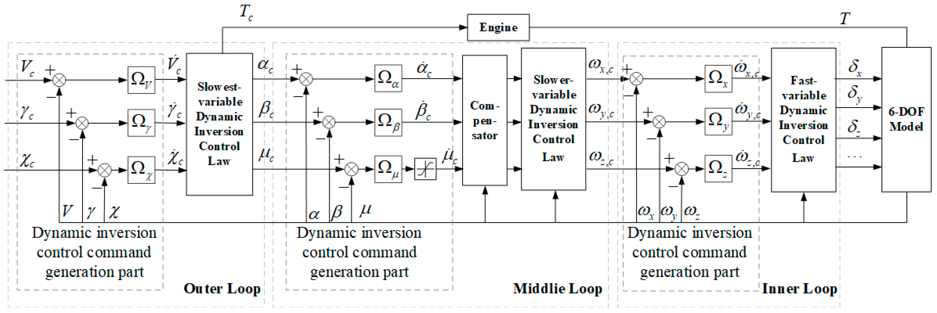
The NDI control law, based on the trajectory command, was designed using the inner, middle, and outer loops. Each layer corresponded to a state variable with different response speeds. The inner loop primarily regulates the three-axis angular rate ω x , ω y , ω z . The control module consists of a fast-variable dynamic inversion command generation module and a corresponding dynamic inversion law. The middle loop controls the relatively slow flight variable, α , β , μ . Its control module includes a slower-variable dynamic inversion command generation module, a nonlinear error compensator, and a dynamic inversion law for the slower variables. The outer loop regulates the slowest-changing system variable, V , γ , χ . It combines command inputs and state feedback to generate the slowest-variable control commands using the dynamic inversion method, ensuring that the vehicle response tracks the commands with the expected dynamic characteristics. The corresponding controller structure is shown in Figure 2. The following describes the structure of the trajectory command-based nonlinear dynamic inversion flight control law in the following order: the inner loop first, then the outer loop, and the dynamic inversion control command generation part first, followed by the dynamic inversion control law. This layered structure is suitable for flying-wing UAV autopilots because trajectory commands can be converted into attitude and actuator commands without requiring onboard pilot intervention. The bandwidths of the inner and middle loops (10.0 rad/s and 2.0 rad/s, respectively; see Table 2) correspond to a time-scale separation ratio of approximately 5:1, ensuring that the fast inner-loop rate dynamics are effectively decoupled from the slower middle- and outer-loop responses; the overall controller structure and its NDO-augmented counterpart are illustrated in Figure 2 and Figure 5, respectively.

3.1.1. Inner Loop Flight Control Law

For the fast-variable control command generation, the inner loop control input command was ω x , c , ω y , c , ω z , c . To obtain the fast-variable control command ( ω ˙ x , c , ω ˙ y , c , ω ˙ z , c ) and ensure that the aircraft response ( ω x , ω y , ω z ) can effectively track the control command, the response characteristics can be designed as first-order dynamic characteristics in the Laplace domain, where s denotes the Laplace operator, expressed as follows:
ω i = Ω i s + Ω i ω i , c
where Ω i ( i = x , y , z ) are the tracking response bandwidths for the three-axis attitude angular rates. Accordingly, the required fast-variable dynamic inversion control instructions ( ω ˙ x , c , ω ˙ y , c , ω ˙ z , c ) to achieve the predetermined tracking characteristics can be derived.
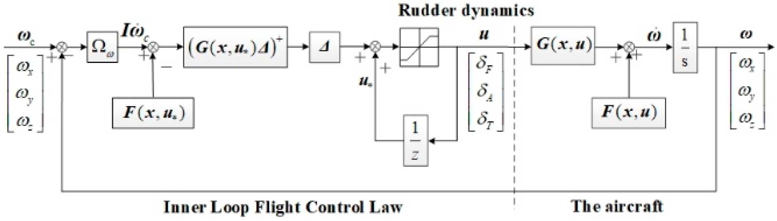
For the fast-variable dynamic inversion control law, the deflections of the inner and outer ailerons ( δ F , δ A ) and wingtip rudders ( δ T ) were derived using the dynamic inversion method.
According to the aircraft’s rotational dynamics equations, the combined external moment required to achieve command ω ˙ c is M r :
M r = I ω ˙ c + ω × I ω
The desired combined external moment M r consists of three components: the stabilizing moment, damping moment, and maneuvering moment generated by the control surfaces. By reasonably controlling the control surface deflections to produce this desired combined external moment, ω ˙ = ω ˙ c can be achieved, ensuring the aircraft motion effectively tracks the input command.
As the UAV standard model lacks thrust vectoring, the combined external moment M r required to achieve the control command ω ˙ c consists primarily of the aerodynamic moment M a . This moment is a function of the current flight state x ( x = [ ω x , ω y , ω z , α , β , μ , V , γ , χ ] T ) and the control inputs u ( u = [ δ a , δ e , δ r ] T ). The aerodynamic moment M a is linearly expanded with respect to the control input u under the current x and previous time input u * :
M r x , u = M a x , u * + M a u x , u * u u *
If we denote:
G x , u * = M a u x , u * F x , u * = M a x , u * ω × I ω
Substituting Equations (16) and (17) into the rotation equation yields:
I ω ˙ = M r x , u ω × I ω = F x , u * G x , u * u * + G x , u * u
To solve the equation for u , it is necessary to ensure that the required ω ˙ c has a solution. In this case, the matrix G always has a pseudoinverse G + that satisfies G G + = I . The control surface deflection solution equation required to meet the given angular acceleration vector change is derived as follows:
u = G + x , u * I ω ˙ c F x , u * + u *
Clearly, substituting Equation (19) into the rotational dynamics equation yields ω ˙ = ω ˙ c , indicating that the input calculated using Equation (19) can drive the system according to a predetermined command.
However, in actual flight, there are physical limitations to the control of surface deflections. When one control surface approaches saturation, whereas others still have available margins, this control method alone may not maximize the control potential of all the control surfaces.
Therefore, the diagonal matrix Δ = d i a g [ δ F , max , δ A , max , δ T , max ] is defined as a weighting matrix where the diagonal elements are the maximum deflection angles of each control surface. By defining u ^ = Δ 1 u and G Δ = G Δ , u ^ represents the ratio of the control surface deflection to the maximum deflection. Accordingly, the control law with weighting matrix Δ can be solved as follows:
u = Δ G x , u * Δ + I ω ˙ c F x , u * + u *
Therefore, after introducing the weighting matrix, the system tends to allocate larger deflections to the control surfaces with higher control effectiveness and larger maximum deflection angles. For control surfaces with smaller allowable maximum deflections, the control inputs are appropriately reduced, and the allocated deflections are smaller than those directly calculated using Equation (19). This improves the utilization efficiency of the control surfaces with low control effectiveness and reduces the occurrence of control surface saturation.
By combining the inner loop control command generation and dynamic inversion control law, and considering the control surface deflection saturation, the inner loop control structure shown in Figure 3 is constructed.

3.1.2. Middle Loop Flight Control Law

The design of the middle loop control law is divided into three steps. First, it is necessary to ensure high-accuracy tracking of the outer loop airflow angle commands ( α c , β c , μ c ) and to generate the corresponding rate-of-change commands ( α ˙ c , β ˙ c , μ ˙ c ) for these angles. Second, a dynamic inversion control law algorithm was designed to convert the airflow rate command into an attitude target command ( ω x , c , ω y , c , ω z , c ). Finally, a mid-loop compensator was designed according to the system performance requirements.
For the middle loop control command generation, similar to the inner loop, to ensure that α , β , μ can track the middle loop input command ( α c , β c , μ c ) well, define x = [ α , β , μ ] T , and design the response characteristics as first-order dynamic characteristics in the Laplace domain (again using s to denote the Laplace operator, as defined in Section 3.1.1) as follows:
x = 2 s + 2 x c
Therefore, the dynamic inversion control command ( α ˙ c , β ˙ c , μ ˙ c ) required to enable the system to achieve the expected response performance can be obtained. In flight trajectory control, the sideslip angle command is typically set to zero.
For the slower variable component of the dynamic inversion control law, the change rate of the aircraft airflow angles ( α ˙ c , β ˙ c , μ ˙ c ) can be determined using the translational dynamics equation. Using dynamic inversion control theory, the translational dynamics equation is expressed as follows:
α ˙ β ˙ μ ˙ = f + g ω x ω y ω z
where f = f α , f β , f μ T , related to the aircraft’s attitude and velocity, and g is a nonlinear matrix related to the airflow angles.
Taking the attitude angular rate command ( ω x , c , ω y , c , ω z , c ) as follows:
ω x , c ω y , c ω z , c = g 1 α ˙ c β ˙ c μ ˙ c f
Substituting this into Equation (22) yields [ α ˙ , β ˙ , μ ˙ ] T = [ α ˙ c , β ˙ c , μ ˙ c ] T , indicating that this angular rate command enables the UAV to follow a given slower variable control command.
If the inner loop dynamics are considered instantaneous, that is, the inner loop is assumed to ensure [ ω x , ω y , ω z ] T = [ ω x , c , ω y , c , ω z , c ] T , then the inversion of the mid-loop’s slower variable dynamics theoretically ensures that the UAV responds as follows:
α , β , μ T = 1 s α ˙ c , β ˙ c , μ ˙ c T
This implies that the middle loop dynamic inversion component, inner loop, and airframe form a closed-loop system that is equivalent to an integrator.
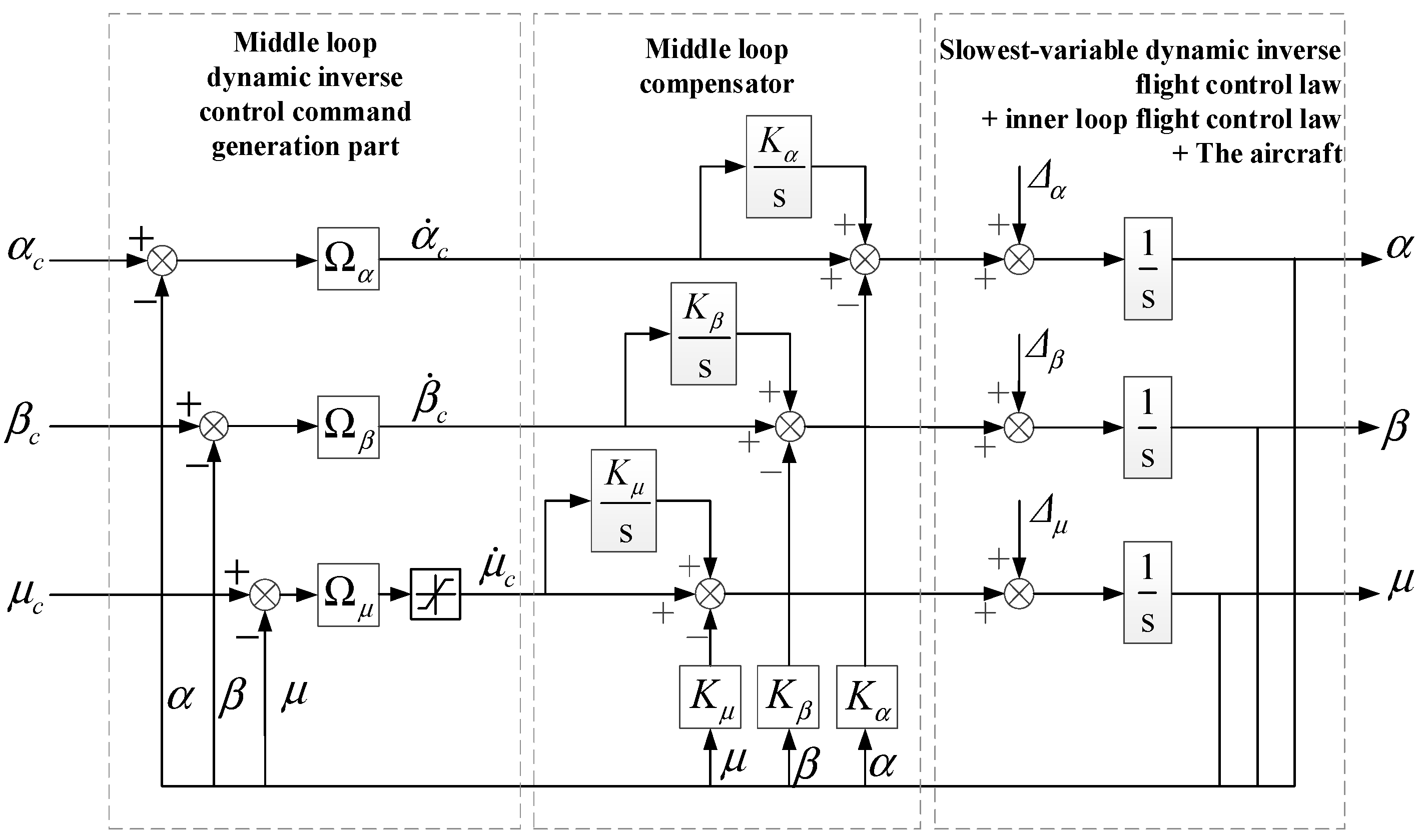
However, in an actual flight control system, the control accuracy can be affected by nonlinear cancellation errors from modeling simplifications and uncertainties as well as by external disturbance forces and moments. Therefore, an integral compensator is added to the middle loop. By defining x = [ α ˙ , β ˙ , μ ˙ ] T , the control signal generated by the integral channel is K ( x ˙ c x ˙ ) / s . Because differential quantities ( [ α ˙ , β ˙ , μ ˙ ] T ) are difficult to measure accurately, the above expression can be rewritten as follows:
x ˙ ε = K s x ˙ c x ˙ = K s x ˙ c K x
The compensator is designed based on the rewritten transfer function. In addition, an excessively large roll angular rate around the velocity vector requires a sufficient yaw rate to suppress sideslip, which leads to an excessive load on the rudder. Therefore, an upper limit constraint must be imposed on μ ˙ c (the command of roll angular rate around the velocity vector). Considering the perturbations and nonlinear cancellation errors, a complete compensatory control structure for the middle loop was constructed, as shown in Figure 4.
In the middle loop control law, Ω α , Ω β , Ω μ is the dynamic bandwidth for the airflow angle tracking response and K α , K β , K μ is the compensator gain. Using the angle of attack ( α ) channel as an example to illustrate the role of the middle loop compensator, the transfer function of the α channel without a compensator is expressed as follows:
α = 2 s + 2 α c + Δ α s + 2
It can be observed that the steady-state value of α is α c + Δ α / 2 (where Δ α is the nonlinear pairwise cancellation error of the α channel). After adding the compensator, the transfer function is as follows:
α = 2 s + 2 α c + s Δ α s 2 + 2 + K α s + 2 K α
At this point, the steady-state value of α is α c . Theoretically, the middle loop compensator, as shown in Figure 4, can eliminate disturbances and pairwise cancellation errors inherent in the nonlinear dynamic inversion method.

3.1.3. Outer Loop Flight Control Law

The design concept for the outer loop dynamic inversion control command generation is similar to that of the inner and middle loops. The control input command is V c , γ c , χ c . To achieve accurate tracking of this input command, defining s = V γ χ T , the dynamic response is designed as a first-order system:
s = 2 s + 2 s c
The slowest-variable dynamic inversion control command V ˙ c , γ ˙ c , χ ˙ c , required to achieve the intended tracking characteristics, can be derived from Equation (28).
Owing to the slow response of the trajectory-related variables, the effects of angular motion and angular rate changes can be neglected in the analysis. By setting the sideslip angle, side force, and forces from the rudder and thrust vectors to zero, the computation for the velocity bank angle command ( μ c ) and the expression for the angle of attack command ( α c ) can be derived as follows:
μ c = arctan V χ ˙ c cos γ V γ ˙ c + g cos γ
m V χ ˙ c cos α cos γ L cos α c sin μ c m V ˙ c D m g sin γ sin α c sin μ c = 0
The angle of attack command can be obtained using Newton’s iterative method. The computed angle of attack command and velocity bank command are then input into the control law loop.
The angle-of-attack solve in Equation (30) is a scalar root-finding problem, and Newton’s method was chosen for its well-known quadratic local convergence; because the underlying aerodynamic-moment/lift relationship is smooth and monotonic over the operating angle-of-attack range, the iteration converges to engineering tolerance within a small, bounded number of steps rather than exhibiting unbounded iteration counts. Each iteration requires only a single evaluation of the residual function and its derivative, i.e., one interpolated lookup of the relevant aerodynamic coefficients plus a small number of arithmetic operations, on the order of a few hundred floating-point operations in total. Given that the flight control computer’s DSP core (a DSP674x-class processor at 456 MHz (Texas Instruments Incorporated, Dallas, TX, USA)) sustains approximately 2746 million floating-point operations per second, a single Newton iteration executes in well under 1 microsecond, and even under a conservative bound of 15 iterations (several times the number actually required for convergence), the total solving time remains on the order of tens of microseconds. This is negligible relative to the 10 ms control-cycle budget set by the 100 Hz update rate at which the airflow-angle sensing chain feeds the flight control computer, leaving ample timing margin for the remaining control-law computations, data acquisition, and command-allocation tasks executed by the FCC within the same cycle.
Beyond the angle-of-attack solver considered above, real-time feasibility must also be established for the complete NDI-DO control law, including the angular-rate, attitude, and trajectory-command loops together with the NDO estimator and control allocation, on representative small-UAV flight-control hardware. All of these tasks are computationally light relative to the Newton solver: they consist of closed-form matrix/vector algebra (state transformations, gain multiplications, and the online model inversion), a bounded number of interpolated aerodynamic-coefficient lookups, and simple first-order observer update equations, none of which involve iterative solving. A conservative estimate places the total operation count for one full control cycle, across all three loops, the NDO, and the control-allocation logic, at no more than a few thousand floating-point operations, which the same FCC core described above executes in a few microseconds, leaving the great majority of the 10 ms control-cycle budget unused by the control-law computation itself. Regarding memory, the control-law code, gain matrices, and interpolated aerodynamic-coefficient lookup tables occupy a negligible fraction of the FCC’s 256 MB of onboard RAM. Regarding sampling rate, the wind tunnel test reported in Section 5.2 was itself executed in real time on this flight control computer at the 100 Hz control cycle described above; the fact that the full closed-loop NDI-DO system, including the Newton-method angle-of-attack solve, ran continuously throughout the reported test at this rate without exceeding its allotted control-cycle budget is itself empirical evidence of real-time feasibility on this class of flight-control hardware, complementing the analytical bound given above.
The thrust command ( T c ) is calculated as follows:
T c = 1 cos α c m V ˙ c + D α c + m g cos γ
Note that the thrust command must satisfy the thrust limitations. The computed thrust command can be input into the engine model to obtain an actual thrust value that complies with these limitations, which is subsequently passed as an input to the aircraft dynamics model.

3.2. Dynamic Inversion Control Law Design Based on NDO

For a flying wing layout of the UAV standard model, it is inevitable that the system will be affected by various disturbances during free-flight in a wind tunnel. Relying solely on the dynamic inversion control law often fails to ensure that a closed-loop system remains linear and time-invariant. Therefore, internal and external disturbances such as system parameter deviations, turbulence, and wind disturbances are uniformly treated as unmatched, centralized disturbances and introduced into the inner loop. This modifies the inner loop closed-loop system equation in Equation (32):
I x ˙ 1 = F ( x 1 , u * ) + G ( x 1 , u * ) ( u u * ) + d 1
where x ˙ 1 = [ ω x , ω y , ω z ] T , u = [ δ a , δ e , δ r ] T , and d 1 represent the centralized disturbance torque containing various model parameter uncertainties and external disturbances.
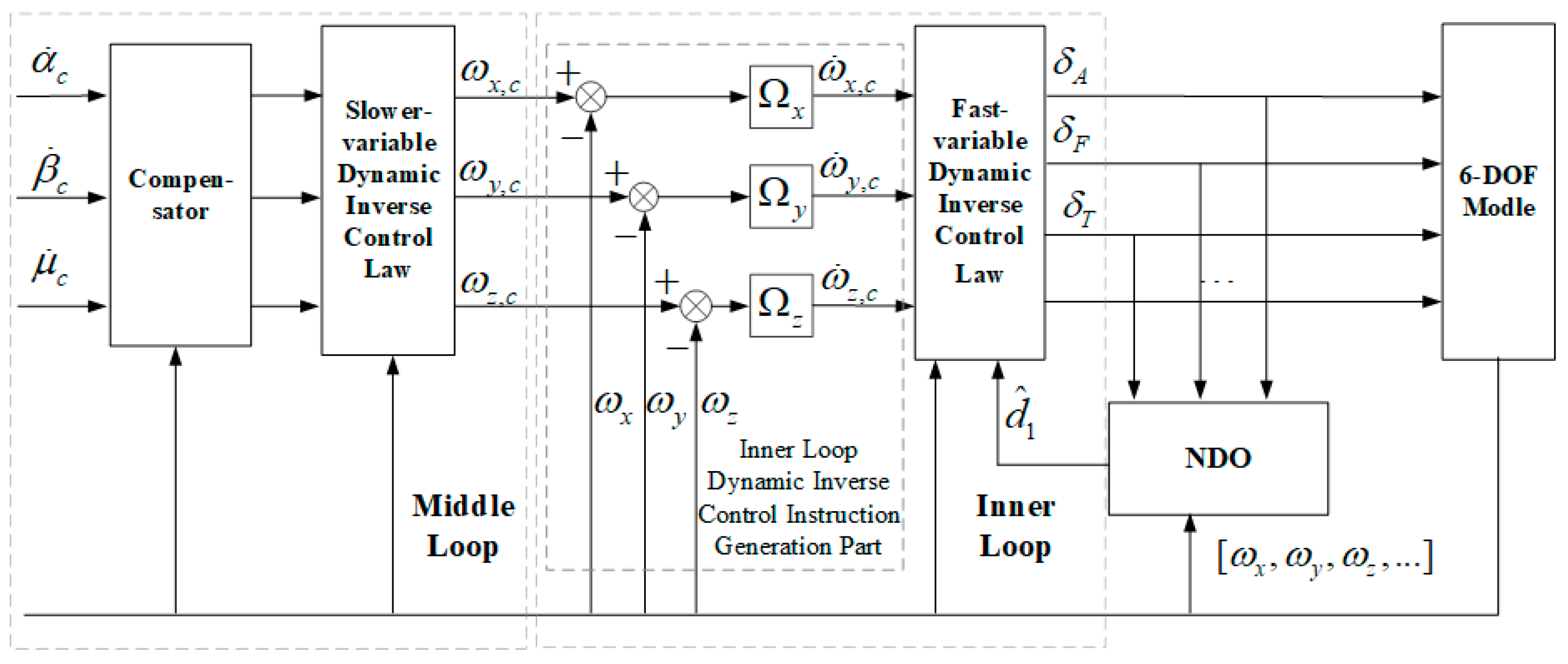
Based on the dynamic inversion control law framework established in Section 2.1, an NDO is added to estimate these centralized disturbances, resulting in an NDI-DO controller, as shown in Figure 5.
Figure 5. NDI controller based on an NDO (NDI-DO).
Drones 10 00601 g005
The core of this control strategy is twofold. First, the disturbance observer performs a real-time estimation of the system’s aggregate disturbance to obtain an estimated value of the centralized disturbance ( d ^ 1 ), which is then introduced into the dynamic inversion control inner loop to perform feed-forward compensation. This composite control architecture can effectively suppress the adverse impact of disturbances on the system output, thereby significantly improving the disturbance rejection and robustness of the control system.
According to literature [46,47], the NDO is designed as follows:
z ˙ d 1 = l ( x 1 ) [ λ ( x 1 ) + z d 1 + F ( x 1 , u * ) + G ( x 1 , u * ) u ] d ^ 1 = z d 1 + λ ( x 1 )
where d ^ 1 is the estimated value of d 1 and z d 1 is the internal variable of the disturbance observer. λ ( x 1 ) is a nonlinear function that must satisfy its design conditions that l ( x 1 ) = λ ( x 1 ) / x 1 .
After obtaining the estimated value of the centralized disturbance from Equation (33) and substituting it into the inner loop dynamic inversion controller in Equation (20), we obtain:
u = Δ G x * , u * Δ + I ω ˙ c F x , u * + d ^ 1 + u *
From the Equations (32)–(34), we can derive the following:
e ˙ d 1 = l ( x 1 ) e d 1 + d ˙ 1
where e d 1 = d 1 d ^ 1 is the disturbance estimation error.
The disturbance estimation error should be asymptotically stabilized to zero by choosing suitable λ ( x 1 ) and l ( x 1 ) to ensure error convergence [46].
Building upon literature [33,48], λ ( x 1 ) can be designed as follows to estimate and compensate for disturbance torque:
λ ( x 1 ) = L I x 1 = l p 0 0 0 l q 0 0 0 l r I x x I x y I x z I x y I y y I y z I x z I y z I z z ω x ω y ω z
where l p , l q , l r are all positive constants, and I is the moment of inertia matrix of the UAV standard model.
The solution of the estimation error dynamics equation is expressed as follows:
e d 1 = e ( t t 0 ) L e d 10 + t 0 t e ( t τ ) L d ˙ 1 ( τ ) d τ
where e d 1 , 0 = e d 1 ( t 0 ) is the initial estimation error.
According to the literature [49], | | e ( t t 0 ) L | | κ 1 e κ 2 ( t t 0 ) holds true. From Equation (37), it further follows that:
| | e d 1 | | | | e t t 0 L | |   | | e d 1 , 0 | | + t 0 t | | e t τ L | | sup t 0 τ t | | d ˙ 1 τ | | d τ κ 1 e κ 2 t t 0 | | e d 1 , 0 | | + t 0 t κ 1 e κ 2 t t 0 d τ sup t t 0 | | d ˙ 1 t | | κ 1 e κ 2 t t 0 | | e d 1 , 0 | | + κ l κ 2 sup t t 0 | | d ˙ 1 t | |
The upper bound of the disturbance observer’s estimation error can be expressed as follows:
lim t + sup | | e d 1 | | κ 1 κ 2 sup | | t t 0 d ˙ 1 t | |
where κ 1 and κ 2 are positive constants determined by the Hurwitz matrix -L.
It follows that, in the zero-input case, the response of the system decays exponentially toward zero. When κ 1 / κ 2 is sufficiently small, the error is also confined to an arbitrarily small neighborhood. To achieve this, the gain matrix elements in Equation (36) must be large to ensure that the observer response is faster than the rate of the disturbance change rate. However, a larger gain value, while improving the disturbance rejection, was found in the actual simulations to extend the system response time for tracking the control command.
Considering control surface saturation, the system equation should be rewritten as follows:
I x ˙ 1 = F ( x 1 , u * ) + G ( x 1 , u * ) [ s a t ( u ) s a t ( u * ) ] + d 1
s a t ( u ) = s a t δ a ( u δ a ) s a t δ e ( u δ e ) s a t δ r ( u δ r ) T
where the saturation characteristics ( s a t j ) are defined by a “dead zone” function.
When the control surface is saturated, the controller in Equation (34) enters a saturated state, which can severely degrade the closed-loop system performance and even trigger instability. Therefore, an anti-windup correction is applied to the disturbance observer equation to improve the system stability and control effectiveness under saturation conditions:
z ˙ d 1 = l ( x 1 ) [ λ ( x 1 ) + z d 1 + F ( x 1 , u * ) + G ( x 1 , u * ) u ] + K s a t [ u s a t ( u ) ] d ^ 1 = z d 1 + λ ( x 1 )
where K s a t denotes the anti-windup gain matrix. To eliminate the effect of actuator saturation, the K s a t can be designed as follows:
K s a t = l ( x 1 ) G ( x 1 , u * )
The anti-windup corrected disturbance observer then becomes:
z ˙ d 1 = l ( x 1 ) [ λ ( x 1 ) + z d 1 + F ( x 1 , u * ) + G ( x 1 , u * ) s a t ( u ) ] d ^ 1 = z d 1 + λ ( x 1 )

4. Comparative Flight Simulation

The calibrated parameters of the controller and observer using the aforementioned dynamic model and control law are listed in Table 2. Preliminary verification of the large-maneuver control performance of the designed NDI and NDI-DO control laws was conducted. A comparative simulation of the Cobra and Split-S maneuvers was performed by constructing a Simulink-based simulation system. Subsequently, the comparative robustness of the two control laws was validated using the Cobra maneuver as an example. The simulation scenarios were selected to evaluate whether the control law can support autonomous recovery and aggressive maneuvering of flying-wing drones without pilot intervention.
To facilitate the performance comparison, simulations were conducted under a wind speed of 30 m/s, with identical control commands for α c , μ c , and β c (where β c was maintained at zero). The control surface deflections are denoted as δ e for the inner elevator aileron, δ a for the outboard aileron, and δ r for the wingtip rudder.

4.1. Comparative Simulation of High Angle of Attack Maneuver Control

4.1.1. Cobra Maneuver

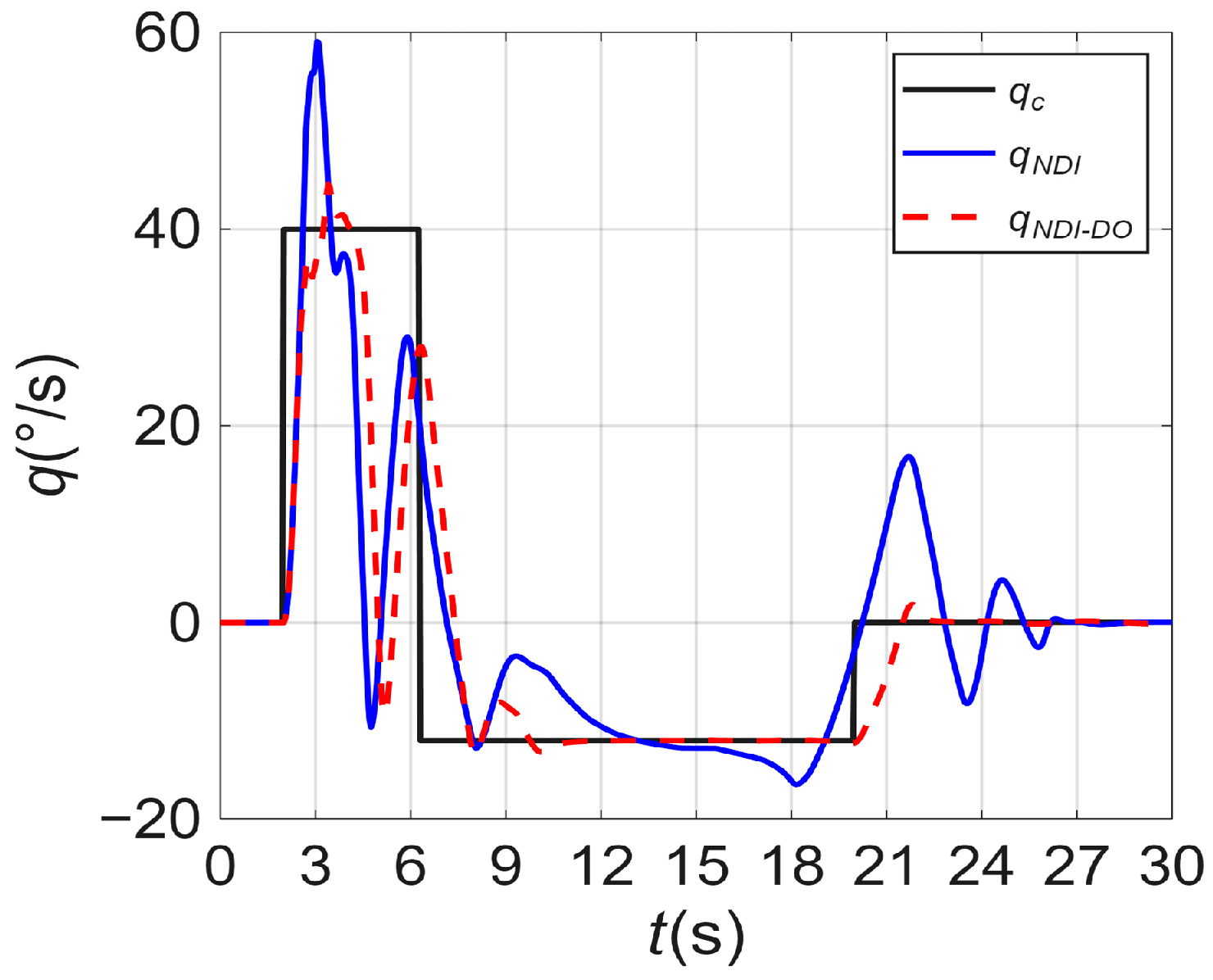
The Cobra maneuver is a typical post-stall maneuver. Because the UAV standard model is commanded through the flight-control computer rather than by direct pilot stick input, its pitch-up or pitch-down motion is realized by tracking the pitch angular velocity command. The closed-loop simulation command tracking curves for the Cobra maneuver under the two control laws and reference conditions of H =   3000 m and V =   200 m/s are shown in Figure 6. The simulation results indicate that both the NDI and NDI-DO control laws effectively track the control commands to complete the Cobra maneuver task and achieve coordinated control surface allocation. The command tracking performance of the NDI-DO control law was superior to that of the baseline NDI, reducing the pitch-rate tracking RMSE by approximately 77.2% while achieving significantly suppressed oscillations and response overshoot. For a UAV, this maneuver represents an envelope-expansion and recovery task performed entirely through automatic command tracking.
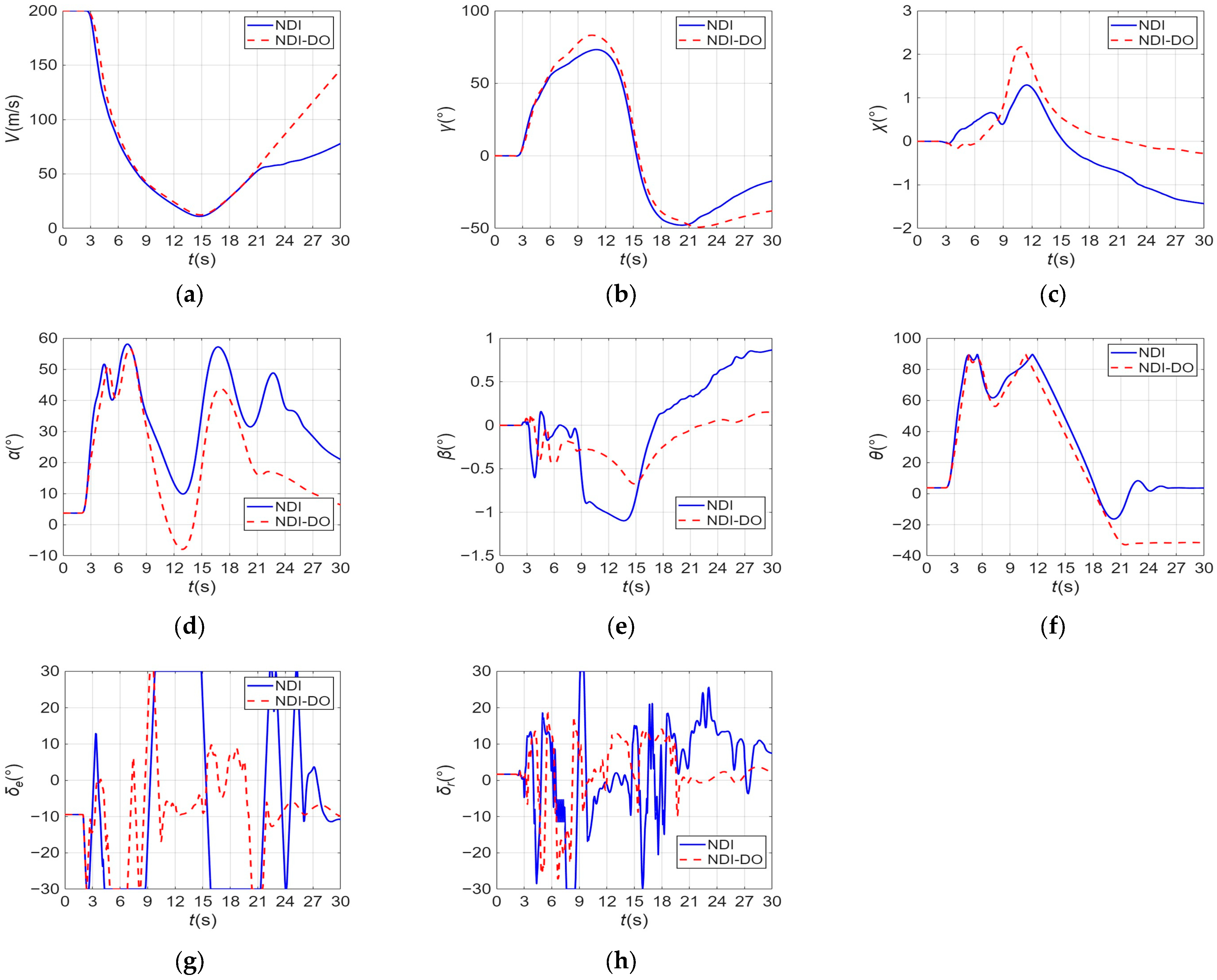
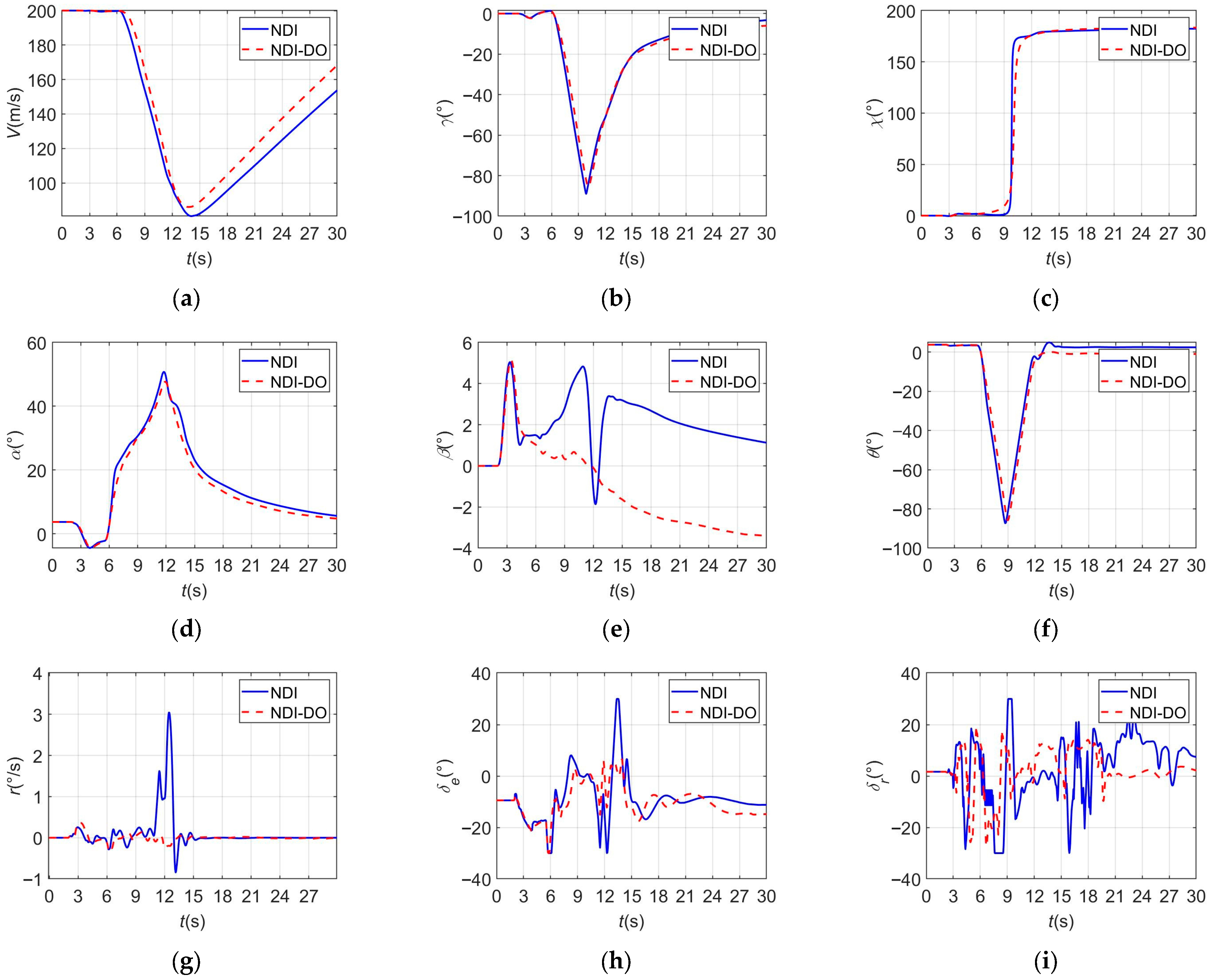
Throughout the Cobra maneuver, the comparative curves of the flight parameters and control surface deflection angles under the two control laws are shown in Figure 7.
Two seconds after the simulation initiation, the pitch angular velocity command q c increased from 0 to 40 ° / s, representing an autopilot-commanded rapid pitch-up input. The inboard elevator aileron deflects upward, generating a pitch-up moment. At this point, strong channel coupling and response overshoot occurred under NDI control, with the UAV model’s maximum pitch angular velocity reaching 59 ° / s. Under NDI-DO control, the maximum pitch rate was approximately 44 ° / s, with significantly less overshoot. Notably, under NDI-DO control, the elevator is not consistently saturated during the pull-up phase, resulting in a more significant longitudinal stability augmentation effect.
At 6 s, the pitch angular velocity command q c decreases from 40 ° / s to −11.6 ° / s, representing an autopilot-commanded pitch-down input, and the angle of attack exhibits an initial downward trend. At 13 s, the horizontal velocity components of the UAV model under both control laws approached 0 m/s and the resulting velocity direction was oriented approximately vertically downward. Therefore, although the q c command is negative, the angle of attack undergoes a secondary increase and does not decrease until 17 s.
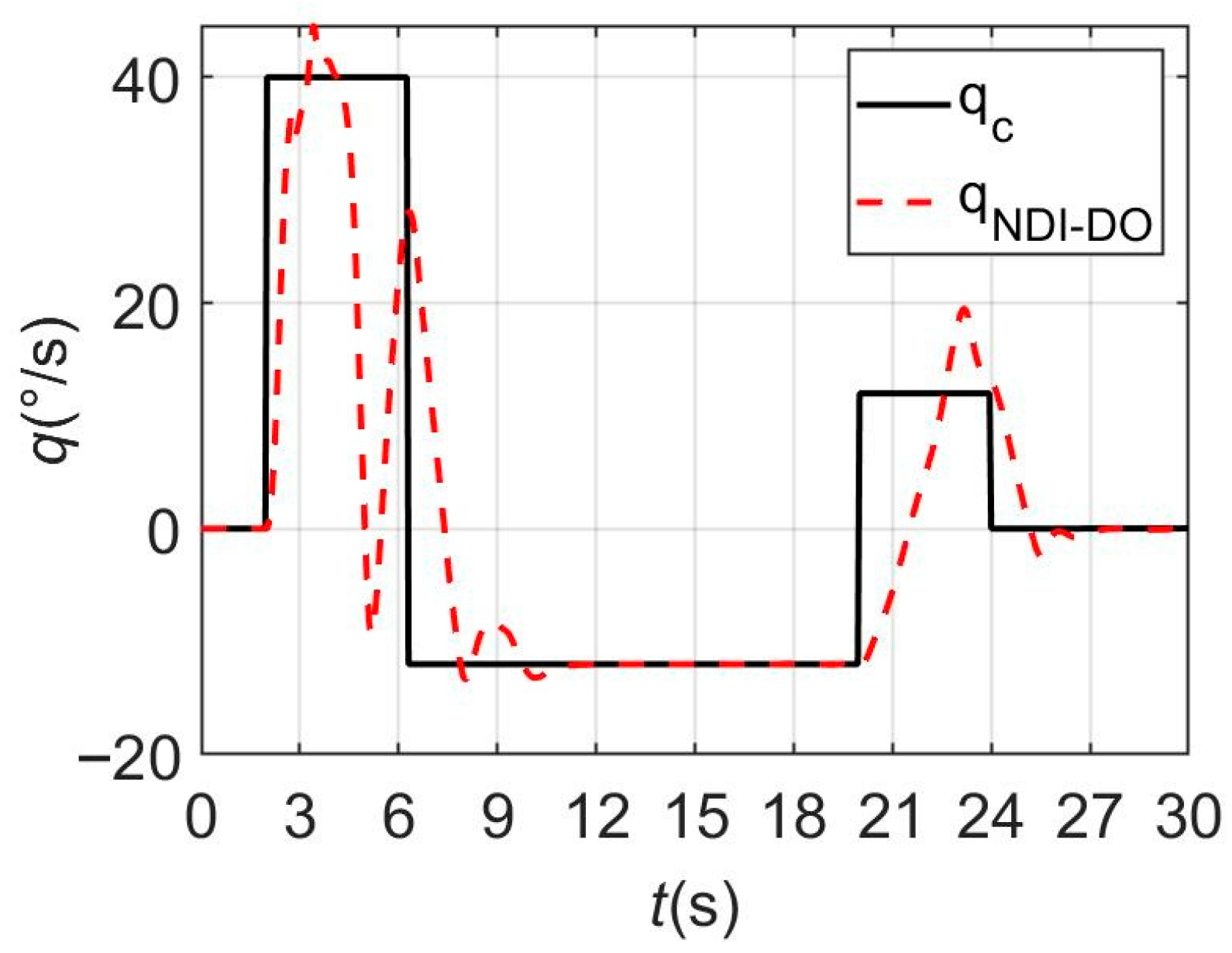
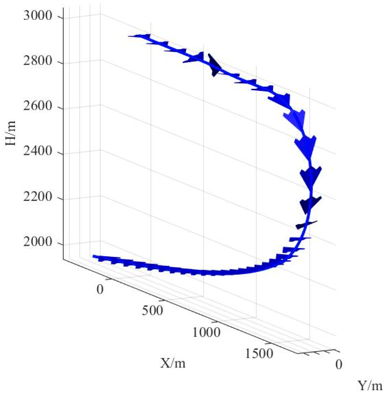
At 20 s, the pitch angular velocity command q c increases from −11.6 ° / s to 0 ° / s, corresponding to an automatic attitude-correction command for the UAV model. Under the NDI control law, the pitch angular velocity response exhibited a large-amplitude positive oscillation, which coincidentally returned the pitch angle to approximately 0°. However, under the NDI-DO control law, the pitch angular velocity response exhibits minimal overshoot and oscillation, and the pitch angle stabilizes at approximately −30°. To rectify this deviation, a pitch angular velocity command was applied that increased to 11.6 ° / s and lasted for 4s. Following this correction, the pitch angle returned to approximately 0 ° , and the pitch angular velocity stabilized at 0 ° / s, thereby completing the Cobra maneuver and restoring the aircraft to a stable state (Figure 8). The corrected trajectory of the Cobra maneuver under the NDI-DO control law is shown in Figure 9.

4.1.2. Split-S Maneuver

In conventional piloted flight, the Split-S maneuver is a standardized large-attitude reversal and descent maneuver that can be used to stress-test flight-control recovery capability. In this study, it is used as a demanding command-tracking and recovery task to evaluate whether the flying-wing UAV can perform rapid roll reversal, dive entry, and recovery through onboard control laws. Under the reference trim conditions of H = 3000 m and V = 200 m/s, the command tracking curves of the Split-S maneuver for the UAV standard model under the two control laws are shown in Figure 10 and Figure 11.
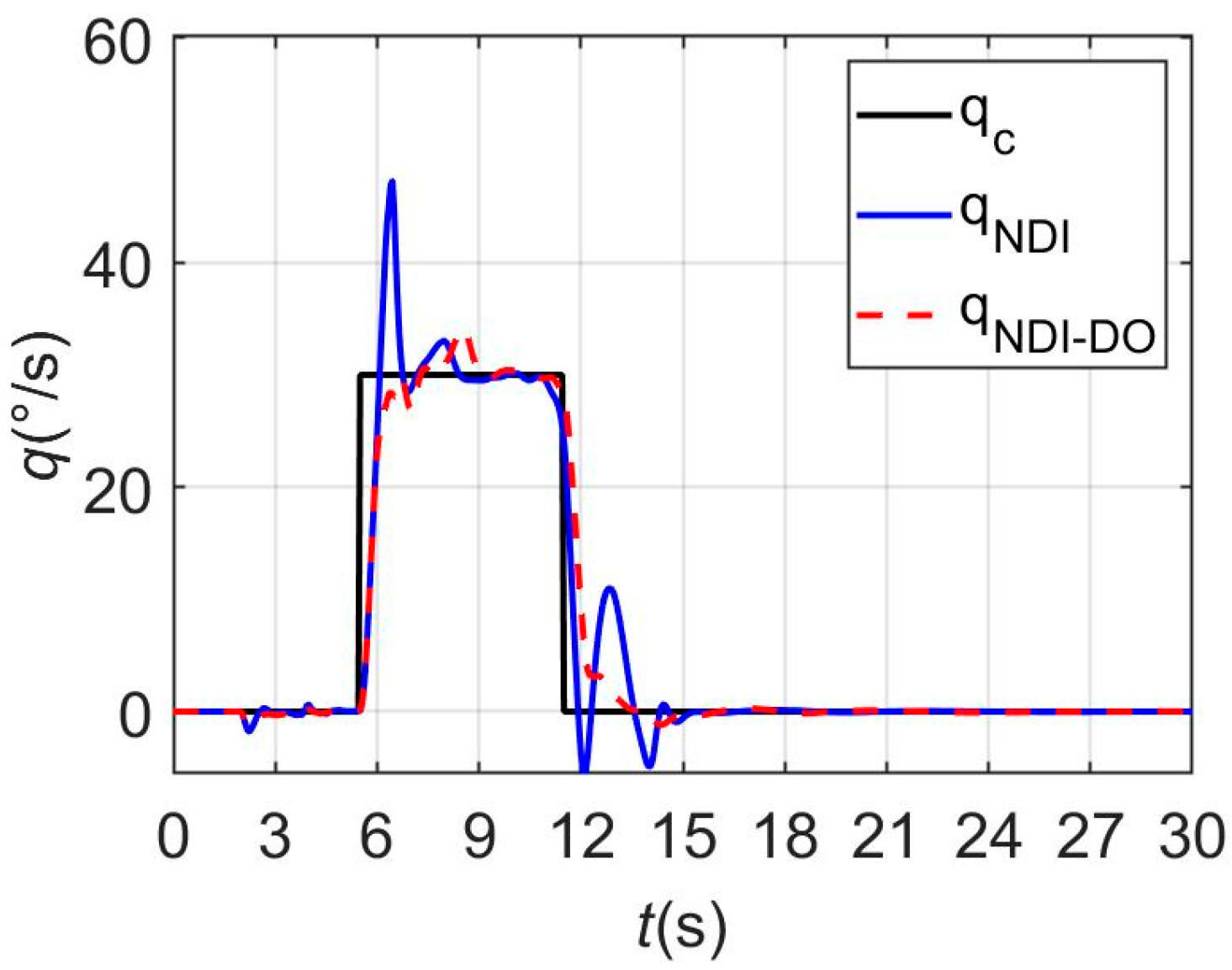
In general, the baseline NDI control exhibits pronounced overshoot and oscillations during angular-rate tracking. In contrast, the NDI-DO scheme provides enhanced tracking fidelity, yielding an RMSE reduction of over 83% for both roll and pitch rate channels. The response curves of the flight parameters and control surface deflection angles for the Split-S maneuver under both control laws are shown in Figure 12.
As shown in Figure 10, 2 s after the start of the simulation, the roll angular velocity command p c increased from 0 to 100°/s. This command drives the UAV model to roll rapidly to the right and enter an inverted flight state at 4 s. Subsequently, at 5.5 s, the pitch angular velocity command q c increases from 0 to 30°/s, driving the UAV model to recover toward normal flight with the smallest feasible turn radius. To increase the angle of attack, the inner elevons of the UAV model must deflect rapidly upward to generate adequate pitch-up moments. It is important to emphasize that during the dive phase, engine thrust must be synchronously reduced to idle to minimize the flight speed increment and mitigate the risk of ground impact due to excessive altitude loss.
The closed-loop simulation trajectory of the Split-S maneuver under the NDI-DO control law is shown in Figure 13, which confirms that the UAV standard model successfully executes the standardized reversal-and-recovery maneuver.

4.2. Robustness Verification

The comparative analysis of high-angle-of-attack maneuvers validates that the integration of NDO provides precise online compensation for mismatched disturbances. The NDI-DO controller restricts the peak angular-rate overshoot to within 10% of the command value and achieves a tracking RMSE reduction of over 77.2%, establishing it as a highly robust control solution for high angle of attack flight regimes. Such robustness is important for civilian drone operations, such as emergency mapping, environmental monitoring, and infrastructure inspection, in which abrupt attitude changes and atmospheric disturbances must be rejected autonomously to maintain safe flight. For example, in the Cobra maneuver (Figure 6), the peak pitch-rate overshoot relative to the 40°/s command was approximately 47.5% under the baseline NDI (peak 59°/s) versus approximately 10% under NDI-DO (peak 44°/s), offering a standardized quantitative measure of the transient-response improvement.
However, as an aircraft enters a flight regime with excessively large angles of attack, the effect of unsteady aerodynamic forces increases. In such cases, the control performance of the nonlinear dynamic inversion may be insufficient to meet the maneuvering requirements, and the aircraft’s motion is prone to divergence. Therefore, the absolute values of the UAV standard model’s three-axis aerodynamic moments are increased by Δ (Δ > 0), and the Cobra maneuver simulation is re-conducted. The robustness of the NDI and NDI-DO control laws was analyzed by comparing the simulation curves before and after aerodynamic moment adjustment.
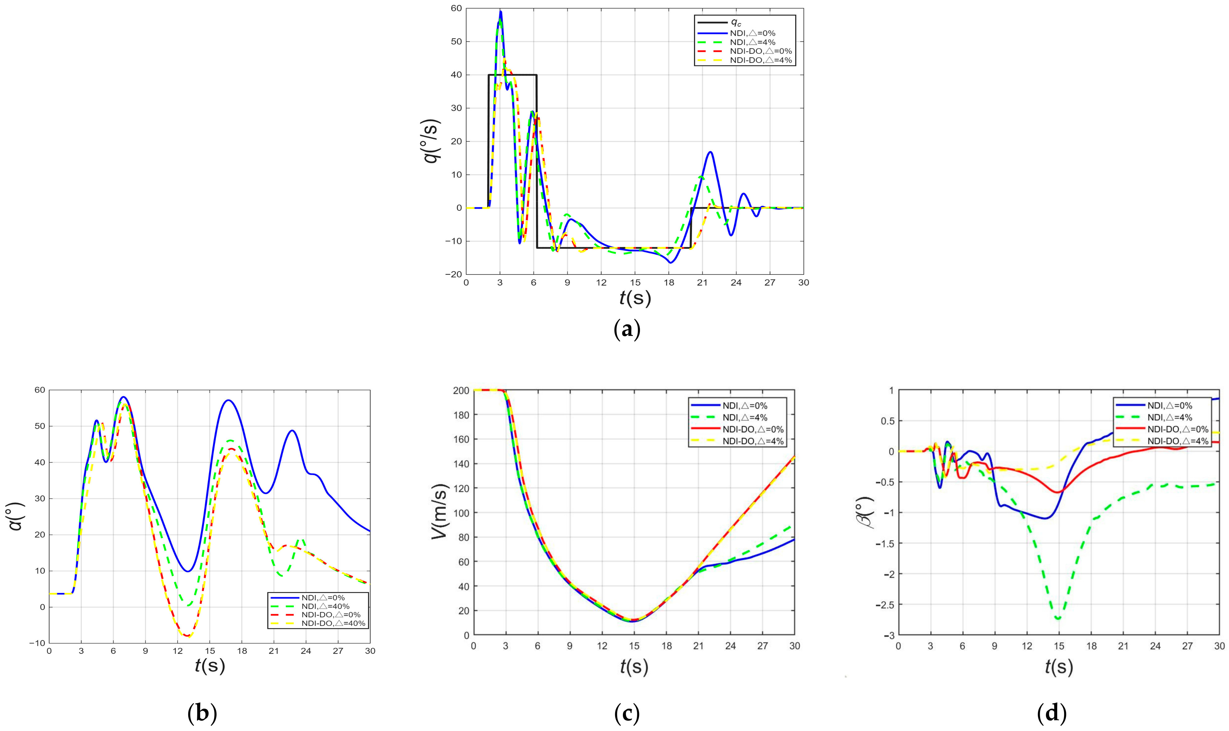
For ease of performance comparison, the Cobra maneuver simulation used a pre-corrected pitch angular velocity command. At the reference trim conditions of H = 3000 m and V = 200 m/s, the simulation results for the Cobra maneuver under both control laws, before and after a 4% increase in the aerodynamic moments, are shown in Figure 14.
It can be concluded that following a 4% increase in the absolute values of the aerodynamic moments, both designed control laws ensure that the aircraft maintains good command tracking characteristics, confirming that the nonlinear dynamic inversion control law exhibits a certain level of robustness. However, under the NDI control law, the dynamic response during the Cobra maneuver differs to a certain extent from that observed prior to the aerodynamic moment perturbation. In contrast, under the NDI-DO control law, the dynamic response exhibits a minimal deviation from the pre-perturbation behavior.
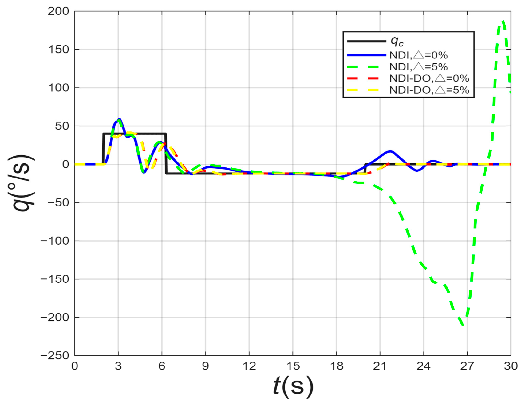
When the absolute values of the UAV model’s inherent aerodynamic moments increased by 5%, as shown in Figure 15, the NDI flight control system was no longer able to track the Cobra maneuver commands. Therefore, the designed NDI control law tolerated a maximum aerodynamic model error of 4% for a standard aircraft model during a Cobra maneuver. For the NDI-DO control law, the lumped disturbance estimated by the disturbance observer includes disturbances induced by aerodynamic parameter deviations; consequently, its command tracking performance remains favorable, and its actual robustness aligns with theoretical expectations. This margin is particularly relevant for UAV deployment because aerodynamic databases for novel flying-wing drones often contain unavoidable interpolation and scaling uncertainties.
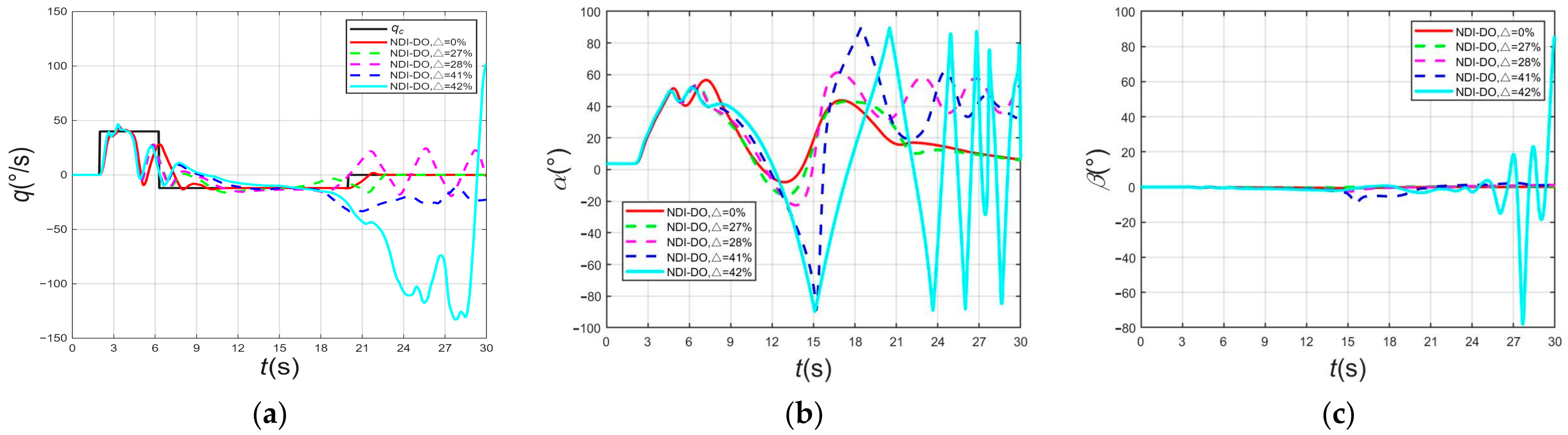
To further investigate the maximum aerodynamic model error tolerable by the NDI-DO control law, the absolute values of the aircraft’s inherent aerodynamic moments were increased by 27%, 28%, 41%, and 42%. The closed-loop simulation results for the Cobra maneuver under the NDI-DO control law are shown in Figure 16.
It can be observed that following a 27% increase in the absolute values of the aircraft’s inherent aerodynamic moments, the NDI-DO control law still ensures that the aircraft maintains good command tracking characteristics with minimal variation in the dynamic response relative to the pre-perturbation state. When the absolute values of the aerodynamic moments are increased by 27–41%, significant oscillations emerge in both the pitch angular velocity command tracking and aerodynamic angle responses; however, the aircraft still does not experience a complete loss of control. The NDI-DO control law fails to track the Cobra maneuver command only when the absolute values of the inherent aerodynamic moments are increased by 42%, and all aerodynamic parameter responses diverge entirely. Therefore, the NDI control law tolerates a maximum aerodynamic model error of 4% for the aircraft during the Cobra maneuver, whereas the NDI-DO control law, which incorporates the disturbance observer, substantially enhances the robustness of the NDI control system. Specifically, it improves the permissible range of aerodynamic parameter perturbations by 23%, and even when the aerodynamic model error reaches 27–41%, the aircraft’s motion does not diverge entirely.
In practical terms, the 41% aerodynamic-moment-perturbation margin tolerated by the NDI-DO control law is expected to cover several realistic sources of aerodynamic-model uncertainty encountered in flying-wing UAV operations, including interpolation and scaling errors in wind-tunnel-derived aerodynamic databases, manufacturing and assembly tolerances relative to the nominal geometry, apparent changes in aerodynamic moments caused by gusts and atmospheric turbulence, and shifts in the center-of-gravity or aerodynamic loading due to interchangeable sensor payloads used in remote sensing, environmental monitoring, or infrastructure-inspection missions. This margin therefore provides a practical safety buffer for the civilian, long-endurance missions targeted by this study, in which onboard controllers must tolerate a degree of aerodynamic-model mismatch without pilot intervention.

5. Wind Tunnel Test Verification of the Control Law for the Flying-Wing UAV Model

This study employs a three-degrees-of-freedom (3-DOF) wind tunnel virtual flight test system to experimentally investigate the high angle of attack control performance of the NDI and NDI-DO control laws in a wind tunnel. Owing to the constraints of the actual wind tunnel conditions, it is difficult to perform the aforementioned high angle of attack maneuver verification. Therefore, a 3-DOF support device was used to mount the unpowered model in the wind tunnel test section, restricting its linear displacement while releasing the degrees of freedom for angular motion (i.e., pitch, roll, and yaw). A wind tunnel test was designed to verify the attitude control performance of the proposed control laws for a UAV standard model during the process in which the angle of attack command increased from 0° to 120° and then returned to 0°, followed by a comparative analysis of the test results and simulation data. The experiment was therefore used as a ground-based validation step before possible free-flight tests of an unmanned flying-wing drone.

5.1. Pre-Test Simulation Validation

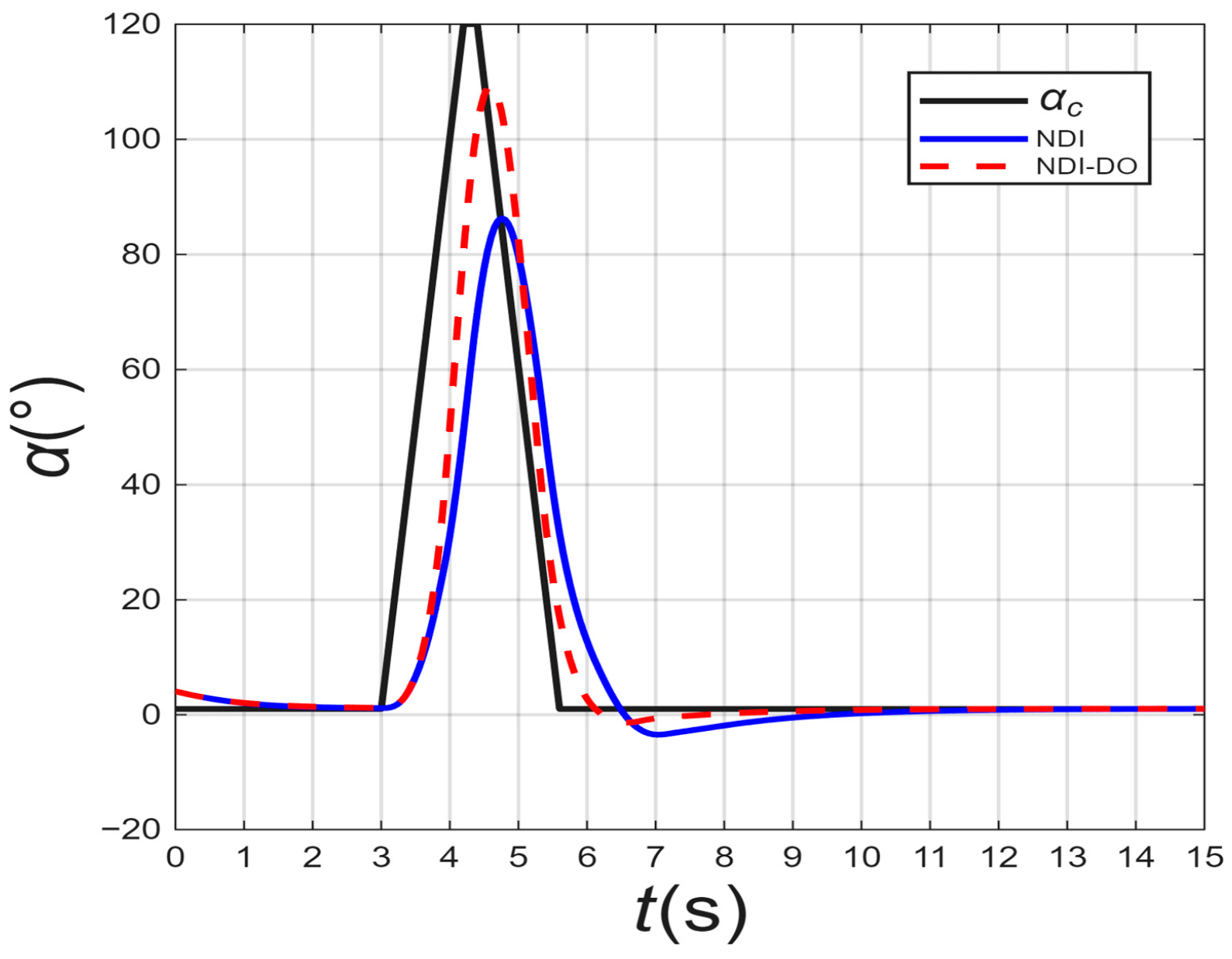
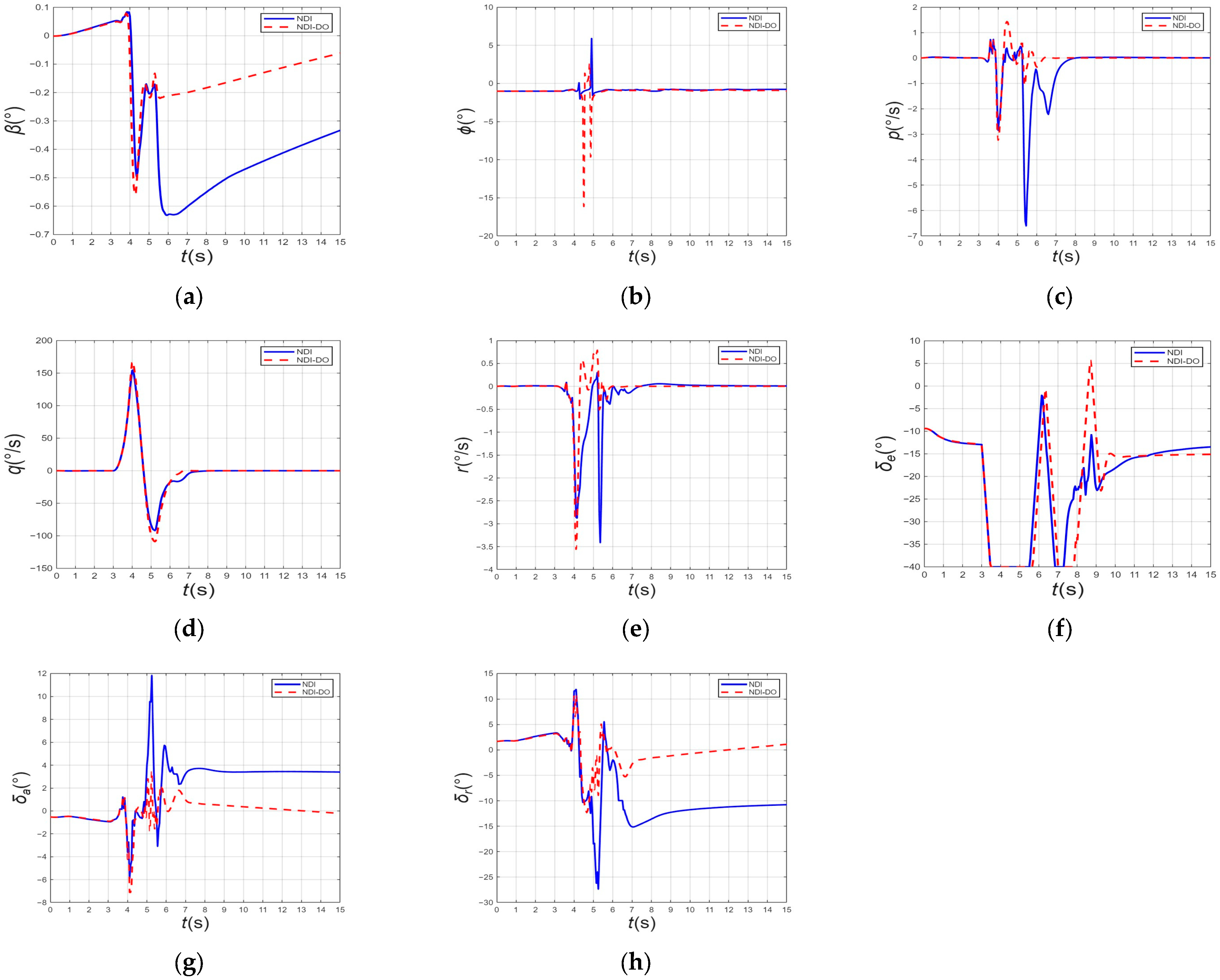
A closed-loop pre-test simulation was conducted using the 3-DOF wind tunnel free-flight dynamic model and the simulation system developed by Simulink. The angle of attack command tracking curves of the UAV standard model under the NDI and NDI-DO control laws are shown in Figure 17, and the corresponding flight parameters and control surface deflection commands during the process are shown in Figure 18.
From the angle of attack command tracking curves shown in Figure 17, it can be observed that both control laws can control the attitude of the aircraft to achieve large variations in the angle of attack and return to a stable state. However, command tracking exhibited a certain time lag. When the maximum angle of attack command was 120°, the maximum angle of attack under the NDI control law reached only 86.26°, whereas it reached 109.28° under the NDI-DO control law. The simulation results demonstrate that, compared with the NDI control law, the NDI-DO control law achieves a larger maximum angle of attack (approaching 110°) during large angle of attack variations, exhibiting a smaller response overshoot, fewer oscillations, and a shorter adjustment time when returning to stability, thus demonstrating superior high-angle-of-attack flight control performance.

5.2. 3-Dof Wind Tunnel Free-Flight Test of the Flying-Wing UAV Model

5.2.1. Test Equipment and Setup

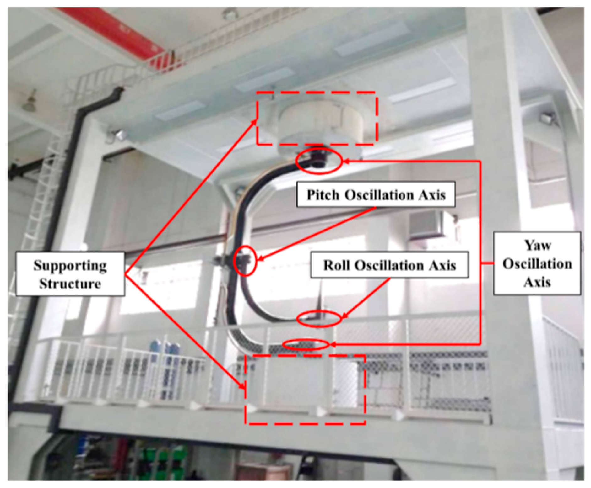
As a link between conventional wind tunnel test and atmospheric flight test, the virtual flight test in a wind tunnel model is an important means for the exploration and demonstration of new aviation concepts and technologies [50]. In the absence of an engine thrust simulation, a 3-DOF support device was used to mount the low-aspect-ratio flying-wing UAV standard model in the wind tunnel test section. This setup restricted the linear displacement of the model while releasing the degrees of freedom for angular motions (roll, pitch, and yaw channels), as shown in Figure 19. Recent advances in wind tunnel gust-generation and free-flight testing rigs for untethered bodies further reflect this growing experimental methodology [51]. This setup provides a repeatable way to evaluate drone control-law behavior under real aerodynamic loads while avoiding the risk and cost of early full-scale flight tests.
The control surface actuators and sensors were installed inside the UAV model. These sensors include vane sensors for measuring the angle of attack ( α ) and sideslip angle ( β ), an Inertial Measurement Unit (IMU) for measuring the attitude rates ( p , q , r ), and an Attitude and Heading Reference System (AHRS) for measuring the attitude angles ( ϕ , θ , ψ ). The flight control computer was placed outside the wind tunnel test section and connected to the onboard avionics via cables. It performs real-time tasks including control law calculations, data acquisition, and command allocation. The sensor and flight-control-computer configuration is consistent with the avionics chain required by autonomous UAV flight-control systems.
The 3-DOF support device constrains linear displacement about the model’s center of rotation while leaving the roll, pitch, and yaw degrees of freedom free, so the reported results characterize attitude-loop control performance under a fixed-position aerodynamic loading condition; they do not capture flight-path-coupled effects such as thrust-induced pitching moment, dynamic-pressure variation with flight-path angle, or gust-induced translational accelerations that would arise in free flight. Extending the present results to full 6-DOF outdoor flight is therefore expected to introduce additional attitude-translational coupling absent from the 3-DOF rig; a dedicated captive-trajectory or outdoor free-flight test, together with the multi-input hardware validation roadmap discussed in Section 6, is identified as a necessary further step before operational deployment. Regarding measurement uncertainty, the angle-of-attack and sideslip vane sensors used in this test have a manufacturer-specified accuracy of 0.3° within ±30°, 0.8° within ±60°, and 2° beyond ±60°; because the high-angle-of-attack excursions reported in this study fall in the beyond-±60° range, the corresponding angle-of-attack measurements carry an estimated uncertainty of approximately ±2°, while the AHRS-based attitude-angle measurements used for the pitch, roll, and yaw response curves carry a specified accuracy of ≤0.5° for pitch and roll and ≤1° for yaw.
During the test, the UAV standard model rotated freely around the spherical hinge center of the support device under the combined effects of wind tunnel airflow, gravity, control-law-based stability augmentation, and flight-operator command input (with linear displacement along the three axes fully constrained). This configuration forms an operator-in-the-loop control law verification and evaluation platform. The flight control law was deployed to the FCC via the main control computer, and the flight operator generated manual intervention commands or standard excitation commands using a control stick to achieve the desired attitude motion of the UAV model. Thus, it can be concluded that the wind tunnel, UAV model, model support, flight control system, and flight operator collectively constitute the verification system, which supports the verification and evaluation of the attitude control law for a UAV standard model. Although operator inputs were used to command the test sequence, the stabilized response was generated by the onboard control law, making the setup relevant to supervised testing of autonomous drone controllers.

5.2.2. Test Results and Analysis

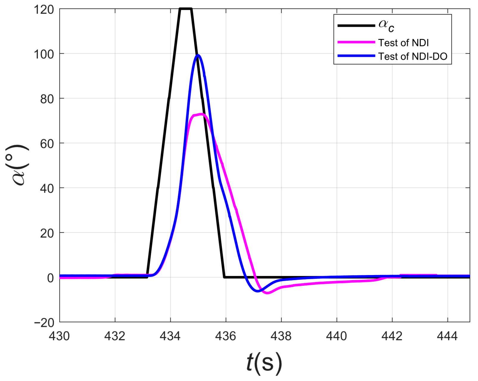
Following the wind tunnel test, only the inner elevon command ( δ e ) was manipulated, with the outer elevon ( δ a ) and wingtip rudder ( δ r ) held at zero deflection. Using the same angle-of-attack command as in the pre-test simulation, high-angle-of-attack flight tests for the NDI and NDI-DO control laws were conducted under 3-DOF free-flight conditions; the comparative tracking curves are shown in Figure 20. This choice reflects a hardware limitation of the present rig rather than a control-allocation restriction: at the time of testing, the actuator and real-time feedback chains for the outer elevon and wingtip rudder had not been integrated to the same reliability standard as the inner elevon channel. Restricting the test to a single input also served a deliberate isolation purpose: low-aspect-ratio flying-wing aircraft have inherently limited yaw authority [7,11], and control-surface effectiveness is known to degrade further at high angle of attack [7], so closing the loop on all three surfaces simultaneously during the extreme excursion studied here (up to 99.19°) could have introduced a lateral-directional divergence unrelated to the pitch-axis NDI-DO law under evaluation. The results reported here therefore validate NDI-DO for single-input, longitudinal angle-of-attack tracking; extending the actuation chain to validate the full multi-input allocation scheme is discussed as future work in Section 6.
This multi-input limitation applies to the wind tunnel hardware validation specifically, not to the control-allocation algorithm: in the 6-DOF simulations of Section 4.1, the wingtip rudder is treated as an active control effector computed online by the NDI-DO allocation law (Figure 7h and Figure 12i), and the architecture already mitigates the platform’s yaw-authority deficiency by design, through the coordinated-turn logic described in Conclusion (1). Hardware validation of the multi-input scheme is therefore a valuable engineering step but is not required to validate the algorithmic contribution reported in this study.
As shown in Figure 20, the maximum angle of attack achieved under the NDI control law during the wind tunnel test was only 72.9°, whereas it reached 99.19° under the NDI-DO control law. The NDI-DO control law exhibited a stronger high-angle-of-attack command tracking performance and required a shorter adjustment time to return to a value near 0° compared with the NDI control law, which is consistent with the previously obtained simulation results. This result substantiates the superiority of the NDI-DO architecture in handling intense nonlinearities within the post-stall regime, expanding the controlled flight boundary to a super-high angle of attack of 99.19° and representing a substantial breakthrough in the high angle of attack maneuverability of flying-wing aircraft. The following analysis focuses on the attitude response performance of the aircraft under the NDI-DO control law. Because the 3-DOF wind tunnel rig constrains linear translation and does not simulate engine thrust, this result is more accurately characterized as an expansion of the controllable angle-of-attack attitude-stability envelope under a fixed-pivot condition, rather than a full flight-envelope expansion involving unconstrained translational flight dynamics; the latter, which for post-stall maneuvers such as the Cobra depends heavily on excess thrust to overcome post-stall drag, is instead supported by the 6-DOF simulation results in Section 4.1, which explicitly include thrust modeling.
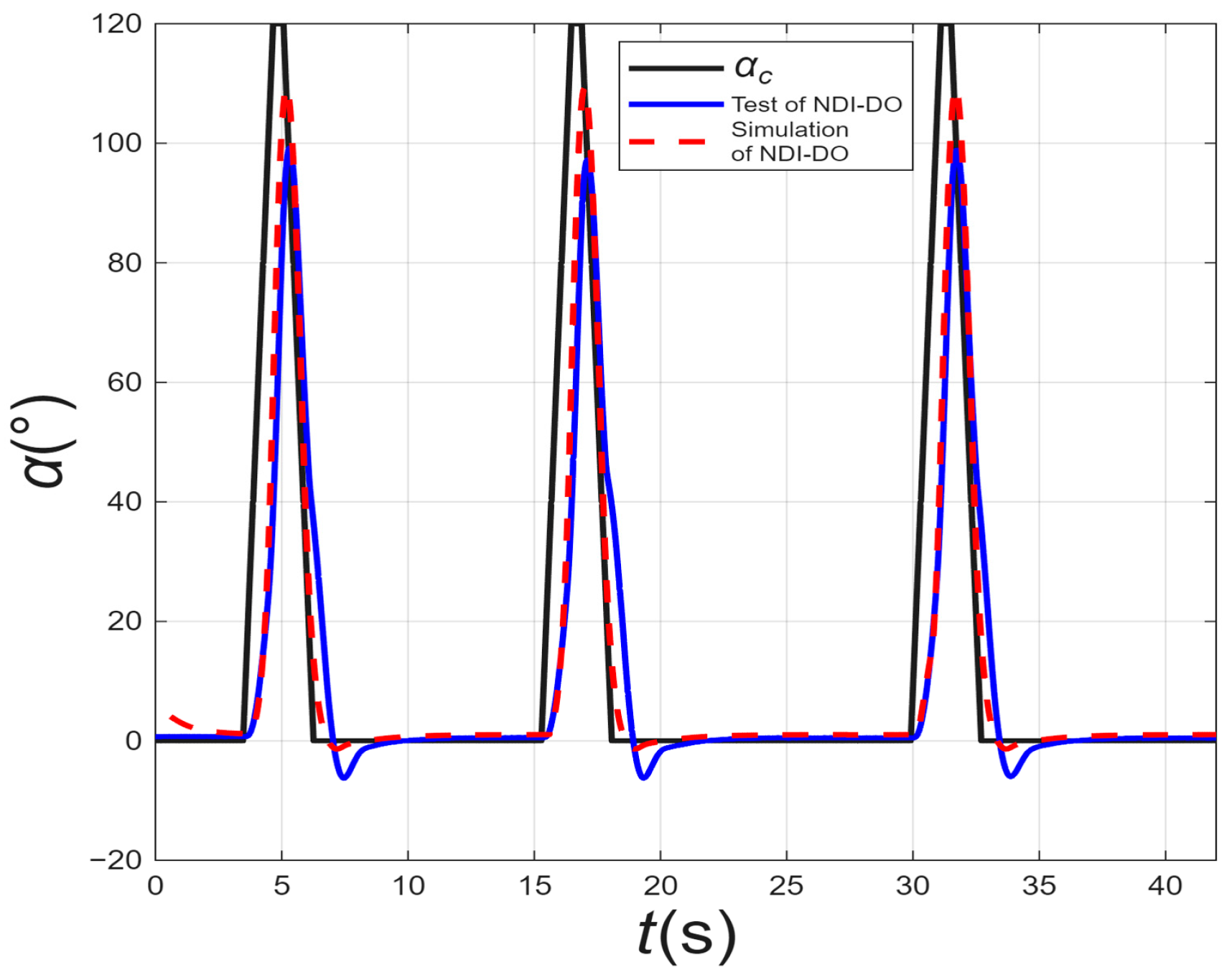
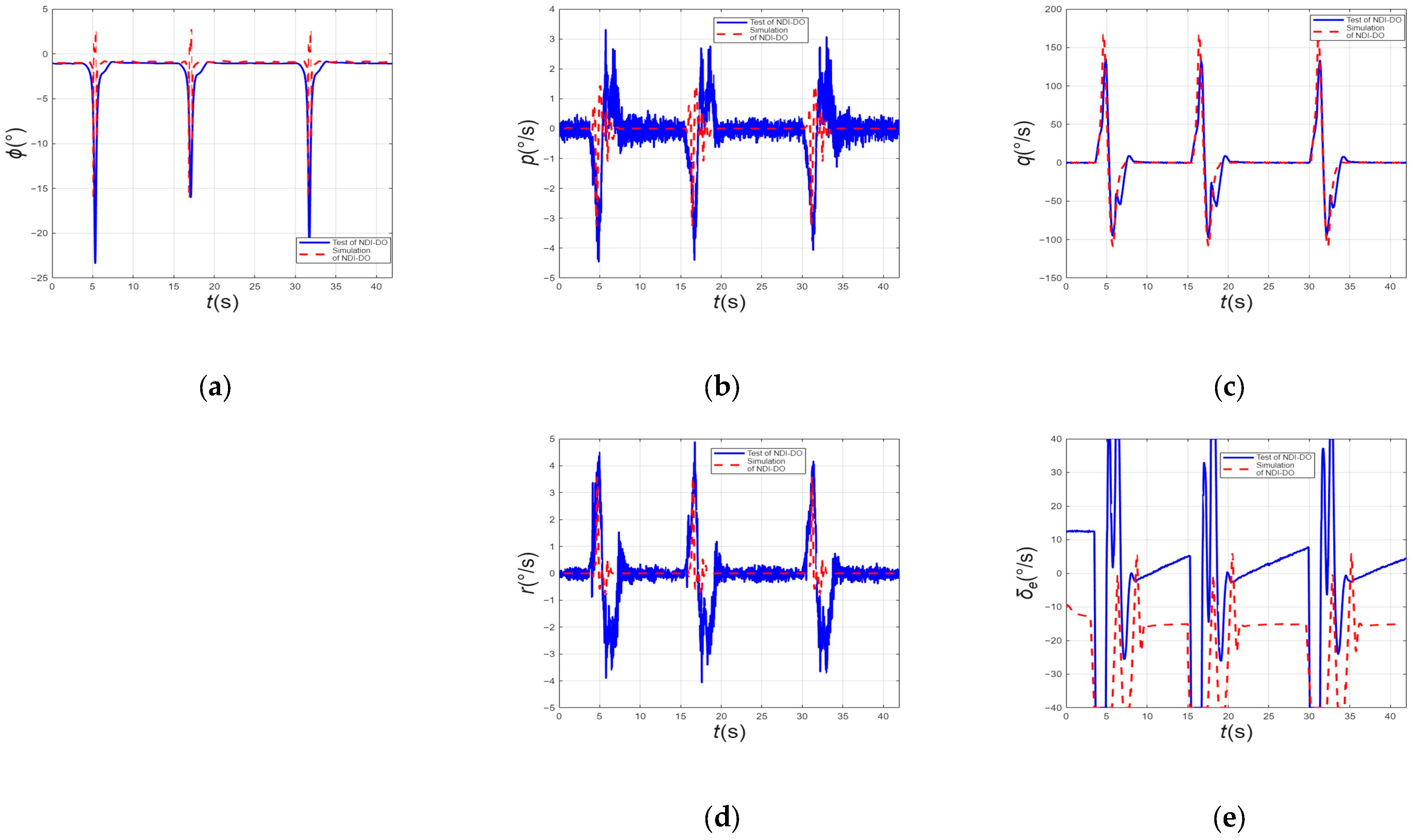
Figure 21 and Figure 22 show the comparative angle of attack command tracking curves, as well as the corresponding flight parameter and inner elevon command curves obtained from the simulation and wind tunnel test under the NDI-DO control law, respectively. To facilitate a comparison with the simulation results, the simulation curves of the angle of attack and flight parameters for the NDI-DO control law are shown in Figure 21 and Figure 22. The time axis of the test data was shifted such that its first-phase command aligned with the simulation data (that is, covering the time interval from 0 s to 42 s). This time shift consisted of a single constant offset applied uniformly to the entire test time series to align the start of the first command phase with the simulation, without any stretching or independent re-alignment of individual response segments; a constant offset by construction preserves the relative timing between the commanded input and the measured response, so the shift does not mask transport delays, phase lags, or actuator latencies in the hardware loop. Indeed, any such delay present in the raw test data is preserved unchanged after the shift and is explicitly reported in this study, where the test response exhibits a longer time lag than the corresponding simulation response (see the following paragraph).
Overall, the test results demonstrated that under the NDI-DO control law, the aircraft exhibited good attitude response performance during the test. Compared to the simulation results, the angle of attack command tracking exhibited good consistency. However, owing to unavoidable disturbances in the test environment, including sensor deviations, measurement noise, aerodynamic interference from the model support, and airflow fluctuations, the control performance of the NDI-DO controller in the flight test was slightly degraded compared to the simulation results. As shown in Figure 18, the peak angle of the attack response in the test was slightly lower than that in the simulation, the time lag was longer, and the overshoot when returning to a stable state was larger. These non-idealities are representative of conditions that a practical drone controller must tolerate during autonomous operation.
In summary, both the simulation and wind tunnel free-flight test results indicate that the NDI-DO control law has superior high-angle-of-attack flight control performance compared to the NDI control law. It can effectively achieve attitude stability augmentation for a low-aspect-ratio BWB standard model during high-angle-of-attack flights in wind tunnel tests. When facing various disturbances under wind tunnel test conditions, the high angle of attack flight control performance of the NDI-DO control law is slightly degraded compared with the simulation results but remains excellent. Therefore, the method provides a feasible ground-test route for evaluating high-angle-of-attack control laws before applying them to flying-wing UAVs.

6. Discussion

The six-degree-of-freedom model developed in Section 2 treats the UAV as a rigid body with fixed inertia and ideal first-order control-surface actuators; aeroelastic coupling and dynamic-stall hysteresis are not modeled, standard simplifications at this vehicle scale. To assess how mass and inertia variations, such as those from payload installation or fuel burn, affect controller robustness, a dedicated simulation sweep scaled the vehicle mass and all three principal moments of inertia ( I x x , I y y , I z z ) by a factor ( 1 + δ ) , with δ ranging from 0% to 80% in 10% increments. Both the NDI and NDI-DO controllers were evaluated at each perturbation level. Neither controller diverged over the entire tested range, and the peak angle-of-attack performance was essentially unaffected by the mass and inertia changes for both controllers. The principal distinction emerges in the post-maneuver settling phase (t = 9~15 s). Table 3 lists the settling-phase root-mean-square error (RMSE) of the angle of attack relative to its value at the end of the simulation window, for both controllers at every tested perturbation level. The NDI-DO controller maintains this settling-phase RMSE within 0.15~1.19° across the entire range, growing only modestly and monotonically with the perturbation, whereas the baseline NDI controller exceeds this upper bound at δ = 10% (1.96°) and at every level from δ = 40% (1.85°) to δ = 80%, rising steadily to a peak of 4.45° at the maximum tested perturbation ( δ = 80%). These results confirm that the disturbance observer effectively compensates inertia-dependent moment errors, keeping the settling-phase response bounded under realistic payload-installation scenarios.
Although a direct quantitative comparison against Active Disturbance Rejection Control (ADRC) and Sliding Mode Control (SMC) was outside the scope of the simulation and wind tunnel campaigns reported here, their expected relative performance can be reasoned about qualitatively from their structural differences with the proposed NDI-DO architecture. ADRC relies on an extended state observer (ESO) to estimate a “total disturbance” from input–output data alone, without an explicit aerodynamic model; this makes it robust to unmodeled dynamics but generally more conservative in bandwidth, since the ESO must be tuned cautiously to avoid amplifying sensor noise, and its disturbance estimate carries no structural information about the underlying aerodynamic nonlinearity. The NDO used here instead leverages the analytically inverted aerodynamic model already required by the NDI law, so its disturbance estimate corrects a known nonlinear model rather than an unstructured input, consistent with the large tolerable aerodynamic-perturbation margin (up to 41%) reported in Section 4.2. SMC achieves robustness through a discontinuous switching term that drives the system state onto a sliding surface, providing strong theoretical robustness guarantees but at the cost of control-signal chattering, which is particularly undesirable for the elevon and wingtip-rudder actuators used here, where high-frequency switching could accelerate actuator wear or excite unmodeled structural modes. NDI-DO instead produces continuous control commands by construction, avoiding this chattering trade-off, at the cost of retaining some dependence on the accuracy of the baseline aerodynamic model.
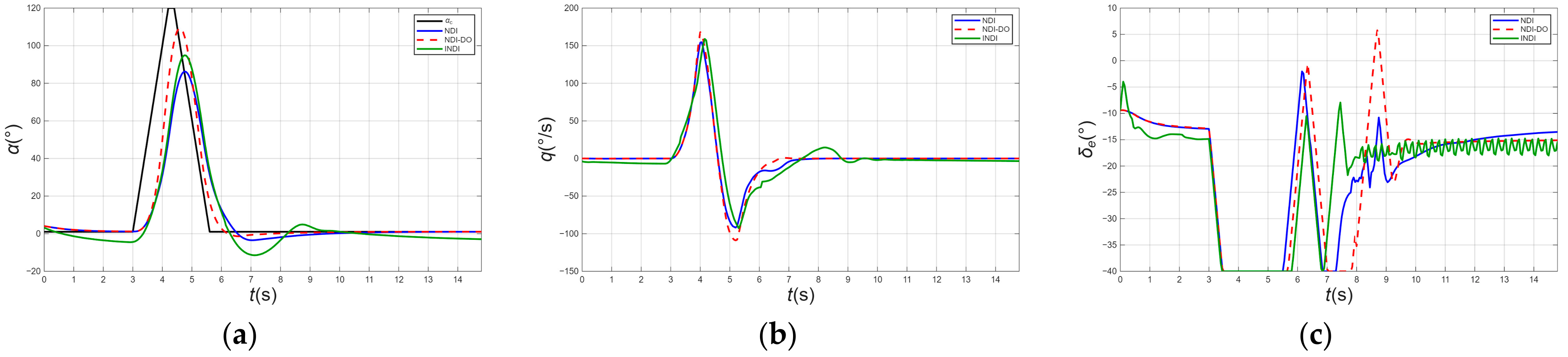
To provide a more direct basis for the choice of NDI-DO over sensor-based incremental alternatives, a simplified Incremental NDI (INDI) controller was implemented in the same six-degree-of-freedom simulation environment and evaluated under the angle-of-attack command tracking task of Section 5.1, identical to that used for the NDI and NDI-DO curves in Figure 21 and Figure 22. In the INDI formulation, the model-computed aerodynamic moment term F is replaced by the inertia-weighted measured angular acceleration I ω ˙ meas , obtained from the rate-gyroscope signal through a first-order differentiating filter with time constant τ = 0.5 s; this value was selected from a sensitivity sweep over τ = 0.01~0.5 s so as not to disadvantage INDI with a poorly tuned filter. All three controllers share the same actuator model, including the ±40° elevator deflection limit, and each saturates this limit during the initial pitch-up transient. Under this command, the peak angle of attack reached 94.9° for INDI, compared with 86.26° for NDI and 109.28° for NDI-DO. The distinguishing behaviour appears in the post-maneuver settling phase (t = 9~15 s): INDI retains a persistent angle-of-attack offset of about 4° and a residual pitch rate of 3.4°/s at t = 15 s, corresponding to a settling-phase RMSE of 2.70°, whereas both NDI and NDI-DO return to within 0.1° and 0.1°/s of the commanded trim values before the end of the window (settling-phase RMSE of 0.54° and 0.15°, respectively). This incomplete recovery reflects INDI’s known sensitivity to differentiation noise: without a dedicated angular-acceleration sensor, which the present hardware does not provide, the incremental formulation loses the algebraic damping supplied by the model-based F term, and its recovery becomes governed by the filter’s tuning. By estimating the aggregate disturbance through the nonlinear disturbance observer rather than by differentiating rate measurements, NDI-DO avoids this dependence and achieves accurate post-maneuver recovery without additional sensor requirements or filter tuning. This result substantiates the preference for NDI-DO over a sensor-based incremental alternative for this UAV class, as shown in Figure 23.
Several extensions are identified as future work. On the hardware side, the real-time actuation chain for the outer elevon and wingtip rudder should be integrated and closed-loop validated, first over the angle-of-attack range already achieved by NDI (0° to 72.9°) before combining it with the more aggressive NDI-DO excursion (up to 99.19°), to experimentally validate the full multi-input control allocation scheme; a dedicated inertia/payload-variation sweep with explicit control-surface actuator dynamics and aeroelastic flexibility, and a captive-trajectory or outdoor free-flight test, would further extend the present rigid-body, 3-DOF results toward full 6-DOF outdoor operation. On the algorithmic side, a rigorous quantitative comparison against ADRC, SMC, INDI, and IBKS implementations under identical simulation and wind tunnel conditions, together with cycle-accurate CPU-load profiling of the deployed control law, would further substantiate the practical advantages of the NDI-DO architecture reported here.
The proposed NDI-DO method targets flight-control safety, envelope protection, and autonomous recovery for the non-weaponized civilian UAV missions described in the Introduction. The reported results are limited to mathematical modeling, simulation, and controlled 3-DOF wind tunnel validation of a scaled standard model; no classified data, sensitive mission data, or security-restricted operational parameters are disclosed.

7. Conclusions

A trajectory-command three-loop dynamic inversion control architecture enhanced by a nonlinear disturbance observer (NDO) was proposed and verified to address the challenges of intense nonlinearity and insufficient yaw authority in low-aspect-ratio flying-wing configurations at high angle of attack. From the perspective of drone applications, the work targets control-law development for unmanned flying-wing platforms that must maintain autonomy and stability in nonlinear post-stall regimes. The primary conclusions are as follows:
(1) A trajectory-command-based nonlinear dynamic inversion (NDI) control architecture was developed, effectively mitigating the inherent yaw control authority deficiencies of flying-wing configurations. For the low-aspect-ratio flying-wing benchmark model, a trajectory-command-to-attitude mapping mechanism was established to incorporate the complex coupling effects of lift, drag, and thrust. By leveraging coordinated turn logic, trajectory-level yaw requirements were successfully transformed into roll-channel control commands. Flight simulations demonstrate that this architecture, integrated with the three-loop time-scale separation principle, maintains high control fidelity under complex high-angle-of-attack maneuvering conditions and eliminates the excessive reliance of conventional control configurations on yaw control torque.
(2) It was confirmed that the synergistic compensation mechanism of the NDO and NDI significantly enhances the robustness margins and tracking accuracy of the control system, enabling controlled flight at super-high angle of attack. Comparative simulation results indicate that the NDI-DO system reduces the state-tracking RMSE by over 77.2% compared to the baseline NDI during high angle of attack maneuvers such as the Cobra and Split-S. By introducing active compensation for model uncertainties and external disturbances, the system robustness in complex aerodynamic environments is substantially improved, with the permissible range of aerodynamic parameter perturbations increased by 23%. More critically, in a 3-DOF wind tunnel free-flight test, the NDI-DO successfully expanded the controlled angle of attack range from 72.9° (baseline NDI) to 99.19°. This result strongly substantiates the superiority of the proposed control architecture in handling intense nonlinearities in the post-stall regime, achieving a substantial breakthrough in the aircraft’s maneuverability. For drone applications, the expanded controllable angle-of-attack range provides a technical basis for safer autonomous recovery and maneuver envelope extension.
(3) The engineering efficacy of the “lumped disturbance” compensation strategy was validated, revealing the robustness of the NDI-DO architecture in real physical environments. To address the drastic aerodynamic perturbations of flying-wing UAVs during unconventional maneuvers, the NDO was utilized not merely as an external disturbance compensator but as a real-time model calibration unit, eliminating the dependence of NDI on precise aerodynamic modeling through feedforward compensation. By unifying sensor noise, support interference, atmospheric turbulence, and model uncertainties into a “lumped disturbance” for online compensation, the NDI-DO successfully bridged the technical gap between idealized simulation and physical experimentation. Wind tunnel tests showed that despite the impact of physical constraints, such as slight lag and peak attenuation in the experimental curves relative to simulation, the NDI-DO maintained the ability to recover stability rapidly following complex maneuvers. This fully substantiates that the proposed NDO-enhanced trajectory-command three-loop NDI architecture possesses high technical resilience and engineering utility in the presence of non-ideal measurements and environmental disturbances. This capability is valuable for unmanned platforms operating without pilot compensation, where onboard controllers must absorb aerodynamic-model errors and environmental disturbances in real time.


Author Contributions

J.W.: Conceptualization, methodology, and writing—original draft; J.L. and Y.L.: Data curation and validation; C.W.: Writing—review and editing and supervision; C.B., S.F. and M.H.: Investigation and resources. All authors have read and agreed to the published version of the manuscript.

Funding

This work was supported in part by the National Natural Science Foundation of China (Grant Number 12272104), in part by the National Natural Science Foundation of China (Grant Number U22B2013), in part by the Key Research and Development Program of Heilongjiang Province (Grant Number 2025ZX01A03), and in part by the Joint Fund of the National Natural Science Foundation of China under Grant No. U25B2090 (Project title: “Design of Continuous Smooth Morphing Trailing Edge and Aerodynamic-Structural Coupling Mechanism for Low-AspectRatio Tailless Flying Wing Aircraft”).

Data Availability Statement

The original contributions presented in the study are included in the article; further inquiries can be directed to the corresponding author.

DURC Statement

Current research is limited to flight-control law design and wind tunnel validation for low-aspect-ratio flying-wing UAVs, which is beneficial for civilian drone safety, autonomous envelope protection, disturbance rejection, remote sensing, environmental monitoring, infrastructure inspection, disaster assessment, and emergency response, and does not pose a threat to public health or national security. The authors acknowledge the dual-use potential of flight-control technologies involving flying-wing UAVs and confirm that all necessary precautions have been taken to prevent potential misuse. The manuscript does not disclose weaponization guidance, targeting functions, payload-delivery design, military mission-planning procedures, classified data, or sensitive operational parameters. As an ethical responsibility, the authors strictly adhere to relevant national and international laws and regulations concerning DURC and advocate responsible deployment, ethical consideration, regulatory compliance, access control for sensitive data, and transparent reporting to mitigate misuse risks and foster beneficial civilian outcomes.
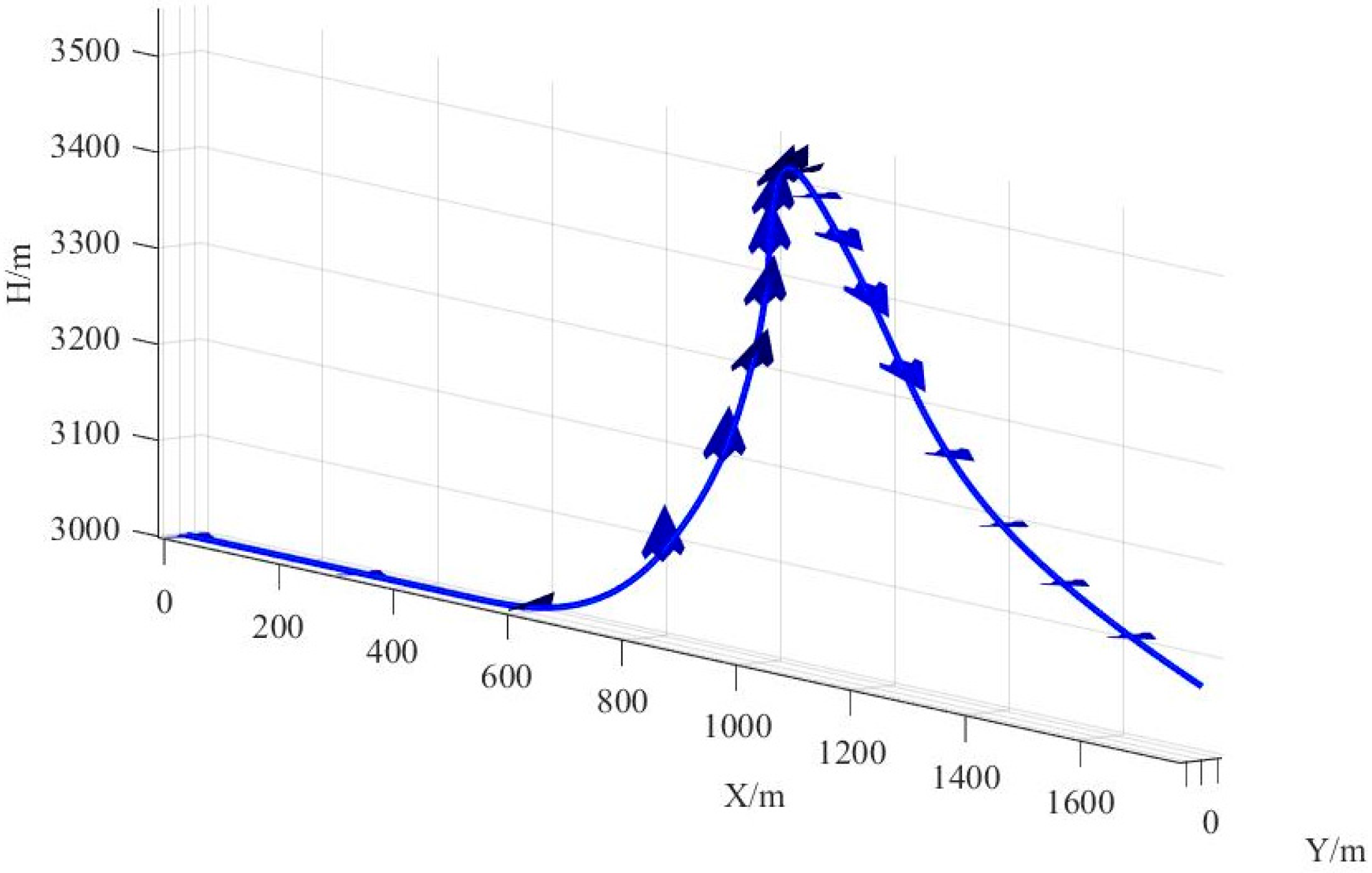
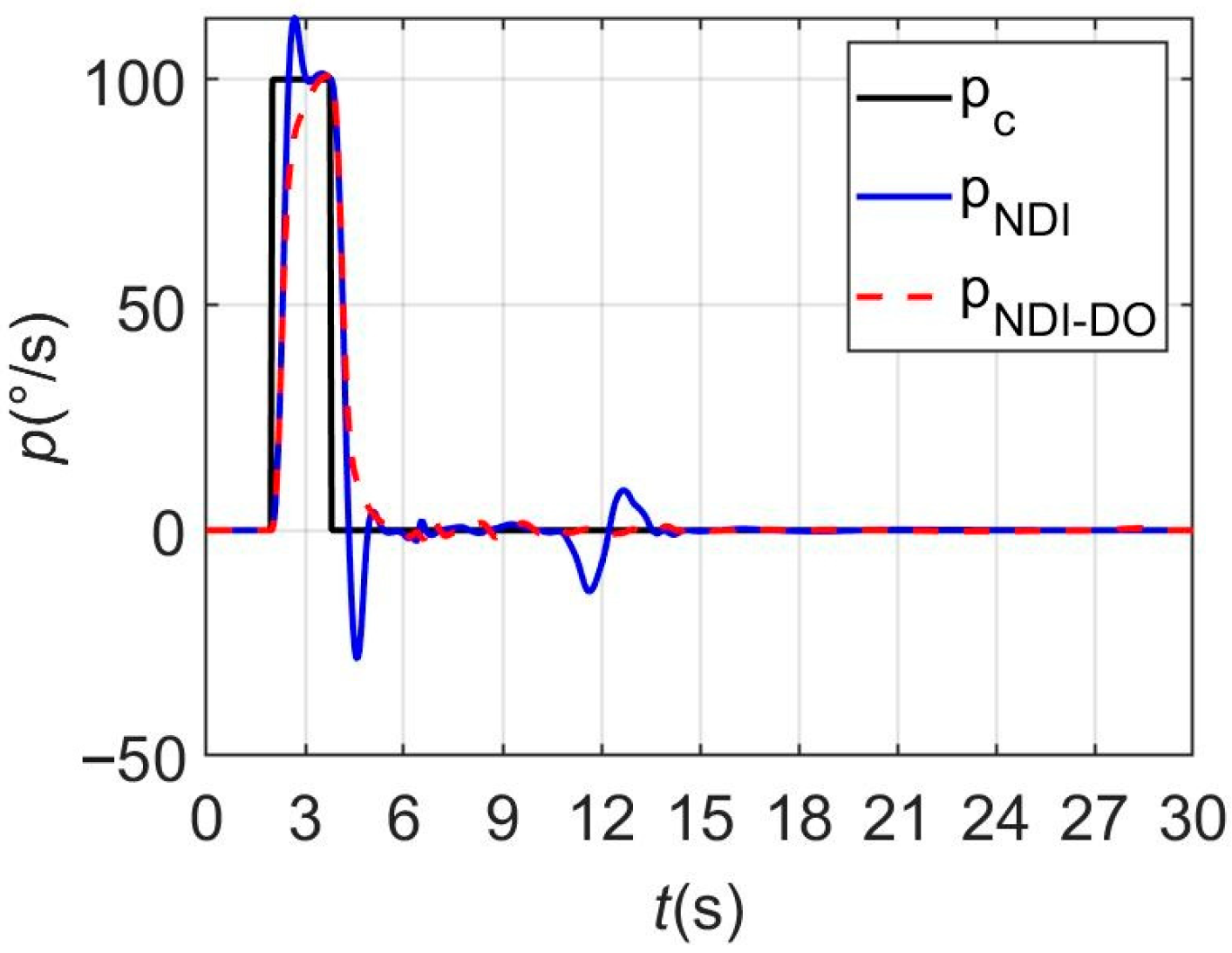
Conflicts of Interest

The authors declare no conflicts of interest.

References

  1. Denisov, V.; Shkadov, L.; Chernyshev, S.B.T. The flying wing concept—The challenge for the future. In Proceedings of the AIAA International Air and Space Symposium and Exposition: The Next 100 Years, Dayton, OH, USA, 14–17 July 2003; pp. 1–11. [Google Scholar]
  2. Lee, G.H. The case for the tailless aircraft. Aeronaut. J. 2016, 50, 872–887. [Google Scholar]
  3. Colgren, R.; Loschke, R. Effective design of highly maneuverable tailless aircraft. J. Aircr. 2008, 45, 1441–1449. [Google Scholar] [CrossRef]
  4. Liebeck, R.H. Design of the blended wing body subsonic transport. J. Aircr. 2004, 41, 10–25. [Google Scholar] [CrossRef]
  5. Liebeck, R.; Page, M.; Rawdon, B. Blended-wing-body subsonic commercial transport. In Proceedings of the 36th AIAA Aerospace Sciences Meeting and Exhibit, Reno, NV, USA, 12–15 January 1998; American Institute of Aeronautics and Astronautics: Reston, VA, USA, 1998; pp. 1–11. [Google Scholar]
  6. Tao, C.G.; Lin, C.J.; Tie, Y.J.; Fan, S.; Liang, T. Controllability evaluation criteria research based on NGAD. Acta Aeronaut. Astronaut. Sin. 2024, 45, 530083. [Google Scholar]
  7. Zhou, Z.; Yu, Y.G.; Liu, G.; Chen, Z.B.; Heng, K.F. Comprehensive study on yaw control characteristic of combined control surfaces of flying wing configuration. Acta Aeronaut. Astronaut. Sin. 2020, 41, 523422. [Google Scholar]
  8. Qin, N.; Vavalle, A.; Le Moigne, A.; Laban, M.; Hackett, K.; Weinerfelt, P. Aerodynamic considerations of blended wing body aircraft. Prog. Aerosp. Sci. 2004, 40, 321–343. [Google Scholar] [CrossRef]
  9. Yang, W. Development of future fighters. Acta Aeronaut. Astronaut. Sin. 2020, 41, 1–12. [Google Scholar]
  10. Wang, G.; Zhang, B.Q.; Zhang, M.H.; Sang, W.M.; Yuan, C.S.; Li, D. Research progress and prospect for conceptual and aerodynamic technology of blended-wing-body civil aircraft. Acta Aeronaut. Astronaut. Sin. 2019, 40, 623046. [Google Scholar]
  11. Bowlus, J.; Multhopp, D.; Banda, S. Challenges and opportunities in tailless aircraft stability and control. In Proceedings of the Guidance, Navigation, and Control Conference; American Institute of Aeronautics and Astronautics: Reston, VA, USA, 1997; pp. 1713–1718. [Google Scholar]
  12. Balas, G.J. Flight control law design: An industry perspective. Eur. J. Control 2003, 9, 207–226. [Google Scholar] [CrossRef]
  13. Ngo, A.D.; Reigelsperger, W.C.; Banda, S.S. Tailless aircraft control law design using dynamic inversion & μ-synthesis. In Proceedings of the IEEE International Conference on Control Applications, Dearborn, MI, USA, 15–18 September 1996; IEEE: Piscataway, NJ, USA, 1996; pp. 107–112. [Google Scholar]
  14. Schumacher, C. Adaptive flight control using dynamic inversion and neural networks. In Proceedings of the Guidance, Navigation, and Control Conference and Exhibit, AIAA, Portland, OR, USA, 9–11 August 1999; American Institute of Aeronautics and Astronautics: Reston, VA, USA, 1999; pp. 1–9. [Google Scholar]
  15. Brinker, J.S.; Wise, K.A. Flight testing of reconfigurable control law on the X-36 tailless aircraft. J. Guid. Control Dyn. 2001, 24, 903–909. [Google Scholar] [CrossRef] [PubMed]
  16. Calise, A.J.; Lee, S.; Sharma, M. Development of a reconfigurable flight control law for tailless aircraft. J. Guid. Control Dyn. 2001, 24, 896–902. [Google Scholar] [CrossRef] [PubMed]
  17. Zhang, L.; Huang, Y.; Zhu, Z.L.; Gao, L.; Chen, F.; Wu, F.; He, M. Virtual flight test of pitch and roll attitude control based on circulation control of tailless flying wing aircraft without rudders. Chin. J. Aeronaut. 2023, 36, 52–62. [Google Scholar] [CrossRef]
  18. Sun, Q.B.; Shi, Z.W.; Geng, X.; Wang, L.S.; Zhang, W.Y. Attitude control of flying wing aircraft without control surfaces based on active flow control. Acta Aeronaut. Astronaut. Sin. 2020, 41, 124080. [Google Scholar]
  19. Zhang, L.; Huang, Y.; Chen, F.Z. Rudderless attitude control flight test based on circulation control of tailless flying wing in pitch and roll axes. Acta Aeronaut. Astronaut. Sin. 2023, 44, 128224. [Google Scholar]
  20. Wang, L.; Wang, L.Y.; Jia, Z.R. Control features and application characteristics of split drag rudder utilized by flying wing. Acta Aeronaut. Astronaut. Sin. 2011, 32, 1392–1399. [Google Scholar]
  21. Li, L.; Wang, L.X. Directional axis flying qualities assessment of low aspect-ratio combat flying wings. Acta Aeronaut. Astronaut. Sin. 2009, 30, 972–978. [Google Scholar]
  22. Cong, B.; Wang, L.X. Low-order equivalent matching methods for aircraft with flying wings. J. Beijing Univ. Aeronaut. Astronaut. 2018, 44, 286–294. [Google Scholar]
  23. Wang, L.X.; Zhang, N.; Yue, T.; Liu, H.L.; Zhu, J.; Jia, X. Three-axis coupled flight control law design for flying wing aircraft using eigenstructure assignment method. Chin. J. Aeronaut. 2020, 33, 2510–2526. [Google Scholar] [CrossRef]
  24. Zhang, Y.H.; Zhang, D.C.; Zhou, Z.W.; Lei, Y.; Li, L. Concept and design of virtual rudder surface aircraft based on circulation control: Review. Acta Aeronaut. Astronaut. Sin. 2024, 45, 629608. [Google Scholar]
  25. Zhang, L.; He, M. Virtual flight test for three-axis decoupling fluidic flight control of tailless flying wing. Chin. J. Aeronaut. 2025, 39, 103811. [Google Scholar]
  26. Xu, B.X.; Feng, L.H. Experimental research on three-axis control of flying-wing aircraft based on active flow control. Chin. J. Aeronaut. 2025, 38, 103443. [Google Scholar] [CrossRef]
  27. Bai, Y.F.; Zou, Q.T.; Huang, R.; Liu, H.; Ran, Y. Aeroelastic control of flexible wing with flying-wing configuration and wind tunnel tests. Acta Aeronaut. Astronaut. Sin. 2025, 46, 231452. [Google Scholar]
  28. Buffington, J. Modular Control Law Design for the Innovative Control Effectors (ICE) Tailless Fighter Aircraft Configuration 101-3; Wright-Patterson Air Force Base: Dayton, OH, USA, 1999. [Google Scholar]
  29. Ngo, A.; Reigelsperger, W.; Banda, S.; Bessolo, J. Multivariable control law design for a tailless airplane. In Proceedings of the Guidance, Navigation, and Control Conference, San Diego, CA, USA, 29–31 July 1996; American Institute of Aeronautics and Astronautics: Reston, VA, USA, 1996; pp. 1–12. [Google Scholar]
  30. Wang, X.; Van Kampen, E.-J.; Chu, Q.; Lu, P. Stability analysis for incremental nonlinear dynamic inversion control. J. Guid. Control Dyn. 2019, 42, 1116–1129. [Google Scholar] [CrossRef]
  31. Wang, C.; Tan, W.Q.; Sun, L.G.; Jiao, J. Flying qualities based time-varying stability augmentation system design for tiltrotor conversion control. Chin. J. Aeronaut. 2024, 37, 366–385. [Google Scholar] [CrossRef]
  32. Chang, J.; Breuker, R.D.; Wang, X.R. Adaptive nonlinear incremental flight control for systems with unknown control effectiveness. IEEE Trans. Aerosp. Electron. Syst. 2023, 59, 228–240. [Google Scholar] [CrossRef]
  33. Smith, J.; Su, J.; Liu, C.; Chen, W.-H. Disturbance observer based control with AntiWindup applied to a small fixed wing UAV for disturbance rejection. J. Intell. Robot. Syst. 2017, 88, 1–18. [Google Scholar] [CrossRef]
  34. Ding, S.; Chen, W.H.; Mei, K.; Murray-Smith, D.J. Disturbance observer design for nonlinear systems represented by input–output models. IEEE Trans. Ind. Electron. 2020, 67, 1222–1232. [Google Scholar] [CrossRef]
  35. An, H.; Wu, Q. Disturbance rejection dynamic inverse control of air-breathing hypersonic vehicles. Acta Astronaut. 2018, 151, 348–356. [Google Scholar] [CrossRef]
  36. Chen, W.H.; Ballance, D.J.; Gawthrop, P.J.; O’Reilly, J. A nonlinear disturbance observer for robotic manipulators. IEEE Trans. Ind. Electron. 2000, 47, 932–938. [Google Scholar] [CrossRef]
  37. Li, S.; Yang, J.; Chen, W.H.; Chen, X. Disturbance Observer-Based Control: Methods and Applications; CRC Press, Incorporated: Boca Raton, FL, USA, 2014; pp. 115–135. [Google Scholar]
  38. Zhang, J.H.; Xiang, J.W.; Li, D.C.; Yang, G.; Di, W.; Zhang, L.; Tu, Z. Anti-Disturbance for ST-VTOL UAV via Sliding Mode Control with Enhanced Observer. Drones 2025, 9, 843. [Google Scholar] [CrossRef]
  39. Sieberling, S.; Chu, Q.P.; Mulder, J.A. Robust flight control using incremental nonlinear dynamic inversion and angular acceleration prediction. J. Guid. Control Dyn. 2010, 33, 1732–1742. [Google Scholar] [CrossRef]
  40. Paul, A.B.; Erik, J.K.; Chu, Q.P. Incremental backstepping for robust nonlinear flight control. In Proceedings of the EuroGNC 2013, 2nd CEAS Specialist Conference on Guidance, Navigation and Control; Springer: New York, NY, USA, 2013; pp. 1444–1463. [Google Scholar]
  41. Sun, L.; Zheng, Z. Disturbance observer-based robust saturated control for spacecraft proximity maneuvers. IEEE Trans. Control Syst. Technol. 2018, 26, 684–692. [Google Scholar] [CrossRef]
  42. Sun, L.G.; Shi, L.W.; Tan, W.Q.; Liu, X. Flying quality based nonlinear flight control law design method for aircraft. Aerosp. Sci. Technol. 2020, 106, 106126. [Google Scholar] [CrossRef]
  43. Valasek, J.; Ito, D.; Ward, D. Robust dynamic inversion controller design and analysis for the X-38. In Proceedings of the AIAA Guidance, Navigation, and Control Conference and Exhibit; AIAA: Montreal, QC, Canada, 2001; pp. 1–11. [Google Scholar]
  44. Menon, P.P.; Lowenberg, M.; Herrmann, G.; Turner, M.C.; Bates, D.G.; Postlethwaite, I. Experimental implementation of a nonlinear dynamic inversion controller with antiwindup. J. Guid. Control Dyn. 2013, 36, 1035–1046. [Google Scholar] [CrossRef]
  45. Herrmann, G.; Menon, P.P.; Turner, M.C.; Bates, D.G.; Postlethwaite, I. Anti-windup synthesis for nonlinear dynamic inversion control schemes. Int. J. Robust Nonlinear Control 2010, 20, 1465–1482. [Google Scholar] [CrossRef]
  46. Yang, J.; Li, S.; Chen, W.H. Nonlinear disturbance observer-based control for multi-input multi-output nonlinear systems subject to mismatching condition. Int. J. Control 2012, 85, 1071–1082. [Google Scholar] [CrossRef]
  47. Chen, W.H.; Ballance, D.J.; Gawthrop, P.J.; Gribble, J.J.; O’Reilly, J. Nonlinear PID predictive controller. IEE Proc. Control Theory Appl. 1999, 146, 603–611. [Google Scholar] [CrossRef]
  48. Chen, Z.; Sun, C.; Cen, F.; Nie, B.; Li, Q. Disturbance Observer Based Dynamic Inversion Control for a Wind Tunnel Free-Flying Test of a Blended-Wing-Body Aircraft; Chinese Automation Congress (CAC): Hangzhou, China, 2019; pp. 5633–5637. [Google Scholar]
  49. Khalil, H.K. Nonlinear Systems, 3rd ed.; Prentice Hall: Upper Saddle River, NJ, USA, 2002; pp. 195–222. [Google Scholar]
  50. Fu, J.Q.; Shi, Z.W.; Gong, Z.; Lowenberg, M.H.; Wu, D.; Pan, L. Virtual flight test techniques to predict a blended-wing-body aircraft in-flight departure characteristics. Chin. J. Aeronaut. 2022, 35, 215–225. [Google Scholar] [CrossRef]
  51. Viola, I.M.; Potnis, A.; Bhattacharyya, S.; Williams, E.J.; Halley, D.; Murphy, D. An accelerating wind tunnel for testing untethered bodies in transverse gusts. Exp. Fluids 2025, 66, 205. [Google Scholar] [CrossRef] [PubMed]
Figure 1. Schematic of low-aspect-ratio flying-wing UAV standard model.
Drones 10 00601 g001
Figure 2. Structure of the NDI control law based on trajectory command configuration.
Drones 10 00601 g002
Figure 3. Inner loop control structure considering control surface deflection saturation.
Drones 10 00601 g003
Figure 4. Middle loop control law structure with a compensator.
Drones 10 00601 g004
Figure 6. Pitch angular velocity command tracking curves of the cobra maneuver.
Drones 10 00601 g006
Figure 7. Cobra maneuver flight parameters and control surface deflection response curves: (a) velocity; (b) Climb angle; (c) Track deviation angle; (d) Angle of attack; (e) Sideslip angle; (f) Pitch angle; (g) Inner elevon; (h) Wingtip rudder.
Drones 10 00601 g007
Figure 8. Corrected pitch angular velocity (q) command tracking curve for NDI-DO.
Drones 10 00601 g008
Figure 9. Corrected trajectory of the cobra maneuver for NDI-DO.
Drones 10 00601 g009
Figure 10. Roll angular velocity (p) command tracking curve.
Drones 10 00601 g010
Figure 11. Pitch angular velocity (q) command tracking curve.
Drones 10 00601 g011
Figure 12. Flight parameter and control surface deflection angle response curves: (a) velocity; (b) Climb angle; (c) Track deviation angle; (d) Angle of attack; (e) Sideslip angle; (f) Pitch angle; (g) Yaw angular velocity; (h) Inner elevon; (i) Wingtip rudder.
Drones 10 00601 g012
Figure 13. Trajectory of the Split-S maneuver under the NDI-DO control law.
Drones 10 00601 g013
Figure 14. Simulation curves of the cobra maneuver before and after aerodynamic moment adjustments: (a) Pitch Angular Velocity Command tracking curve; (b) Angle of attack; (c) Velocity; (d) Sideslip angle.
Drones 10 00601 g014
Figure 15. Pitch angular velocity command tracking curves.
Drones 10 00601 g015
Figure 16. Simulation curves of the cobra maneuver with different increments in aerodynamic moments: (a) Pitch Angular velocity; (b) Angle of attack; (c) Sideslip angle.
Drones 10 00601 g016
Figure 17. Angle of attack command tracking curve.
Drones 10 00601 g017
Figure 18. Flight Parameter and Control Surface Deflection Command Response Curves: (a) Sideslip angle; (b) Roll angle; (c) Roll angular velocity; (d) Pitch angular velocity; (e) Yaw angular velocity; (f) Inner elevation; (g) Outer elevation; (h) Wingtip rudder.
Drones 10 00601 g018
Figure 19. 3-DOF wind tunnel flight test setup.
Drones 10 00601 g019
Figure 20. Comparative angle of attack command tracking curves from wind tunnel tests.
Drones 10 00601 g020
Figure 21. Angle of attack command tracking curves.
Drones 10 00601 g021
Figure 22. Flight parameter and control surface deflection command response curves: (a) Roll angle; (b) Rolling angular velocity; (c) Pitch angular velocity; (d) Yaw angular velocity; (e) Inner elevation deflection command.
Drones 10 00601 g022
Figure 23. Angle-of-attack command tracking comparison of NDI, NDI-DO, and simplified INDI under a common 120° angle-of-attack command pulse: (a) angle of attack; (b) pitch rate; (c) elevator deflection.
Drones 10 00601 g023
Table 1. Basic configuration parameters.
ParameterSymbolValueUnit
Wing spanb0.9m
Mean aerodynamic chordc0.8m
Roll-axis moment of inertia I x 0.2 k g · m 2
Pitch-axis moment of inertia I y 0.5 k g · m 2
Yaw-axis moment of inertia I z 0.7 k g · m 2
Table 2. Controller and observer parameters.
ParametersNDINDI-DO
Ω x , Ω y , Ω z 10.0, 10.0, 10.010.0, 10.0, 10.0
Ω α , Ω β , Ω μ 2.0, 2.0, 2.02.0, 2.0, 2.0
K α , K β , K μ 0.4, 0.4, 0.40.6, 0.6, 0.6
l p , l q , l r N/A3.0, 3.0, 3.0
Table 3. Post-maneuver settling-phase angle-of-attack RMSE (deg) across the mass/inertia perturbation sweep (angle-of-attack tracking maneuver, t = 9~15 s window).
δ (%)NDI Settling-Phase RMSE (Deg)NDI-DO Settling-Phase RMSE (Deg)
00.540.15
101.960.43
201.130.38
300.870.59
401.850.84
502.521.04
602.840.97
703.421.02
804.451.19
Disclaimer/Publisher’s Note: The statements, opinions and data contained in all publications are solely those of the individual author(s) and contributor(s) and not of MDPI and/or the editor(s). MDPI and/or the editor(s) disclaim responsibility for any injury to people or property resulting from any ideas, methods, instructions or products referred to in the content.