Three-Dimensional Dynamic UAV Threat Assessment Using Approach Directionality and Historical-Trend Correction for Multi-Asset Protection

Highlights

What are the main findings?

• A three-dimensional pairwise UAV–asset threat matrix is developed by integrating spatial proximity, vertical approach, directional alignment, historical trends, and adaptive smoothing.
• Simulations show that the method substantially reduces noise-induced score fluctuations and unnecessary ranking switches while maintaining competitive identification accuracy and response delay.

What are the implications of the main findings?

• The matrix representation supports asset-specific UAV prioritization in many-to-many monitoring scenarios.
• The method is interpretable, computationally lightweight, and does not require large labeled datasets, making it suitable for real-time safety monitoring.

Abstract

In multi-asset UAV safety monitoring, dynamic threat assessment is challenged by delayed recognition of changes in the potentially threatened asset and unstable threat rankings under noisy observations. This paper proposes an interpretable three-dimensional dynamic threat assessment method integrating approach directionality, historical trend correction, and adaptive exponential moving average smoothing. Each UAV-protected asset pair is treated as an assessment unit to construct a many-to-many threat matrix. A basic threat score is first derived from UAV type, three-dimensional closing velocity, distance, altitude difference, and vertical approach motion. Approach directionality is then characterized using the geometric alignment between the UAV velocity and the bearing to each protected asset, with optional attitude and reachability information. The temporal trend of directionality is estimated from historical observations to capture persistent changes in approach tendency, while adaptive smoothing balances responsiveness to genuine threat transitions against suppression of noise-induced fluctuations. Comprehensive simulation experiments, including three-dimensional discrimination, Monte Carlo evaluation, observation noise, latency, missed detections, clutter, difficult motion conditions, and ablation studies, demonstrate that the proposed method provides accurate and timely threat identification while substantially improving score and ranking stability. The resulting framework offers an interpretable and computationally efficient basis for multi-UAV threat prioritization and safety-oriented situational awareness.

1. Introduction

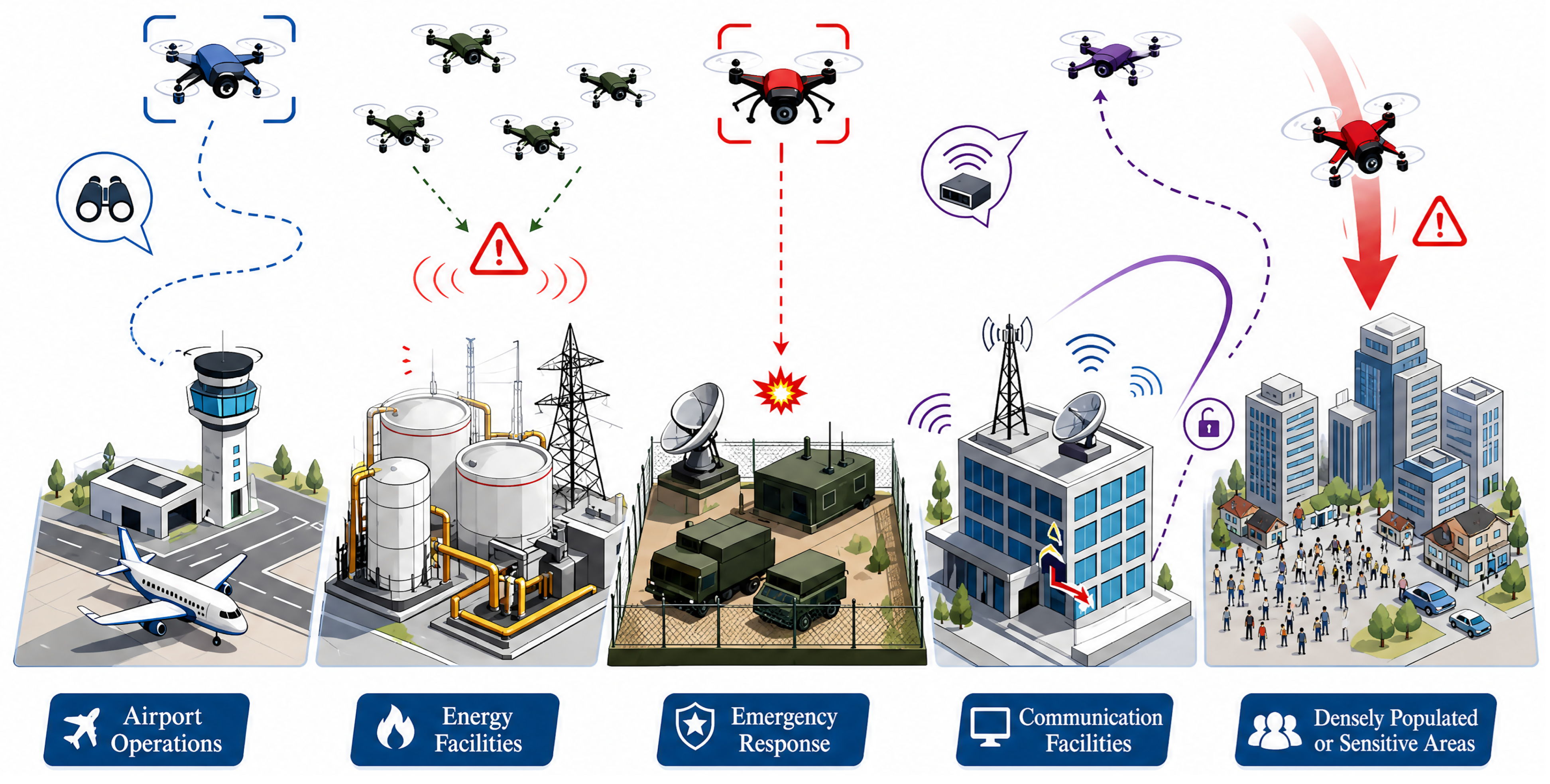
In recent years, unmanned aerial vehicle (UAV) platforms have been widely used in civilian applications such as inspection, mapping, logistics, communication relay, and emergency rescue, owing to their low cost, high maneuverability, ease of deployment, and flexible payload configurations [1,2,3]. However, unauthorized, non-cooperative, or abnormal UAV activities may disrupt airport operations, interfere with emergency response, affect energy or communication facilities, and create safety hazards in densely populated or sensitive areas, as illustrated in Figure 1. Compared with conventional aerial targets, small UAVs usually exhibit a small radar cross section, low flight altitude, flexible velocity variation, and complex maneuvering patterns, which make UAV detection, tracking, identification, and dynamic risk assessment highly challenging. Therefore, dynamic risk assessment for multi-UAV and multi-asset protection scenarios has become an important component of low-altitude airspace safety monitoring, critical infrastructure protection, and public-safety-oriented situational awareness [4,5,6,7,8].

In a typical UAV safety monitoring and protection process, threat assessment lies between target detection/tracking and safety response resource allocation, where the system generally involves a series of functional stages including detection, identification, tracking, threat assessment, warning, mitigation, and response prioritization [9,10]. Its role is to evaluate the threat level posed by different UAVs to different protected assets based on UAV motion states, platform attributes, spatial positions, and potential approach intentions, and to further generate a threat ranking. Accurate threat assessment can assist a protection system in prioritizing the mitigation of high-risk targets, thereby avoiding resource waste and decision-making delays. Conversely, if a threat assessment model fails to identify a shift in the asset potentially at risk in a timely manner, or if threat rankings fluctuate frequently due to noise disturbances, safety response may be delayed and protection effectiveness may be degraded. In particular, in multi-asset protection scenarios, the threat posed by the same UAV to different protected assets may vary significantly, while the same protected asset may simultaneously be threatened by multiple UAVs. Therefore, simply providing an overall threat level for each UAV is no longer sufficient for precise defense requirements. It is necessary to establish a many-to-many threat relationship model between UAVs and protected assets.

Existing threat assessment methods can be broadly categorized into evidence reasoning [11], fuzzy reasoning [12,13], Bayesian network [14], multi-attribute decision making [15,16,17], cloud model [18], neural network-based methods [19], and other learning-based approaches [20].

Table 1. Comparison of typical threat assessment methods in terms of their suitability for multi-asset scenarios: direction/trend information, multi-target matrix output, and data dependence, noise handling and interpretability.

Method	Direction/Trend Information	Multi-Asset Matrix Output	Data Dependence	Noise Handling	Interpretability
Evidence reasoning	Not considered	Not explicitly supported	Relies on prior knowledge	Uncertainty modeling	Traceable reasoning process
Fuzzy reasoning	Not considered	Limited support	Relies on expert experience	Membership functions	Rule-based interpretability
Bayesian network	Indirectly reflected by conditional probabilities	Limited support	Relies on prior data	Probabilistic framework	Clear causal relationships
Multi-attribute decision making	Generally not explicitly modeled	Limited support	No labeled data required	Depends on weight stability	Transparent modeling process
Cloud model	Not considered	Not explicitly supported	Relies on sample data	Considers both fuzziness and randomness	Interpretable cloud droplet distribution
Neural network	Implicitly learned by attention mechanisms	Supported with appropriate architecture	Requires large amounts of labeled data	Depends on training coverage	Relatively weak interpretability; additional tools are required
Learning-based methods	Partially considered through feature learning	Limited support	Requires large amounts of labeled data	Depends on training data coverage	Model-specific; additional tools often required

compare typical threat assessment methods in terms of direction/trend information, multi-asset matrix output, data dependence, noise handling, and interpretability.

In recent years, intention recognition, trajectory prediction, and risk assessment technologies have attracted extensive attention in intelligent transportation, air traffic management, and unmanned system safety. Related studies have shown that motion direction, velocity variation trends, and historical trajectory information can effectively reflect the future behavioral tendency of a target [21,22,23]. In UAV safety monitoring scenarios, when a UAV performs a turning approach, deceptive maneuver, or target redirection, the angle between its velocity direction and different protected assets changes continuously. If a model can capture such a variation trend in directionality, it may identify a shift in the asset potentially at risk before the UAV has completed its heading adjustment. In contrast, models relying only on instantaneous states often respond only after the UAV has clearly pointed toward a new target, resulting in a relatively large detection delay.

In addition, practical UAV safety monitoring systems typically rely on multi-source sensors, such as radar, electro-optical devices, radio-frequency sensing systems, and acoustic arrays, to obtain UAV state information [24,25,26]. These observations are inevitably affected by measurement noise, target occlusion, trajectory jitter, short-term frame loss, and estimation errors. If a threat assessment model is overly sensitive to instantaneous observations, threat values and ranking results may exhibit high-frequency fluctuations or frequent switching, which may further lead to unstable resource prioritization. Existing studies have indicated that smoothing filters, temporal fusion, and state estimation methods can effectively improve the stability of dynamic decision-making systems [27]. However, a fixed smoothing coefficient often struggles to balance rapid response and stable output: excessive smoothing may delay intention recognition, whereas insufficient smoothing cannot effectively suppress noise. Therefore, adaptively adjusting the smoothing strength according to UAV motion states is a key issue in dynamic threat assessment.

To address the above problems, this paper proposes an approach-directionality- based dynamic threat assessment method for multi-asset protection scenarios. The proposed method takes each UAV-protected asset pair as the basic assessment unit. First, a basic threat value is constructed by integrating UAV type, closing speed, altitude, and distance. Then, the angular relationship between the UAV velocity direction and the bearing direction of each protected asset is introduced to define an instantaneous approach directionality factor. Furthermore, a trend correction factor is constructed using the linear variation slope of the historical directionality sequence, so as to enhance or suppress the current directionality. Finally, an adaptive exponential moving average mechanism is introduced to obtain a smoothed threat matrix that balances dynamic response capability and temporal stability. Based on this threat matrix, the UAV threat ranking for each protected asset and the potential approach tendency of each UAV toward different protected assets can be obtained simultaneously.

The main contributions of this paper are summarized as follows.

• A three-dimensional UAV–protected asset threat matrix model is proposed for multi-asset low-altitude safety monitoring. By taking each UAV–protected asset pair as the basic assessment unit, the proposed method represents many-to-many threat relationships in matrix form and enables protected-asset-specific UAV prioritization.
• A three-dimensional directionality modulation and trend-correction mechanism is proposed. It jointly considers altitude difference and vertical approach velocity, thereby improving the discrimination of UAVs with similar scalar threat factors but different spatial approach tendencies. In addition, the historical trend slope of approach directionality is used to dynamically amplify or suppress the current directionality, thereby avoiding static bias when no clear trend exists.
• A dynamic threat correction and smoothing framework is introduced by combining directionality trend correction with adaptive exponential moving average smoothing. The historical directionality trend is used to capture temporal threat evolution, while the adaptive smoothing mechanism balances response sensitivity and temporal stability, thereby reducing noise-induced fluctuations and unnecessary ranking switches.
• The effectiveness and robustness of the proposed method are systematically validated through comprehensive simulation experiments covering vertical- approach discrimination, static and dynamic Monte Carlo evaluation, noise robustness, parameter sensitivity, observation degradation, difficult cases, computational efficiency, and ablation of three-dimensional factors and optional modules.

The remainder of this paper is organized as follows. Section 2 reviews related studies on counter-UAV threat assessment, approach tendency recognition, multi-attribute decision making, and dynamic smoothing. Section 3 presents the proposed approach-directionality-based dynamic threat assessment model in detail. Section 4 provides the simulation settings and experimental result analysis. Section 5 concludes this paper and discusses future research directions.

2. Related Work

2.1. Counter-UAV Threat Assessment

In recent years, the safety and security risks posed by small unmanned aerial vehicles in low-altitude airspace and critical infrastructure protection have become increasingly prominent, creating a growing need for reliable threat assessment in counter-UAV systems. Castrillo et al. [24] systematically reviewed the detection, identification, tracking, and neutralization processes of counter-UAV systems and pointed out that threat determination should integrate multi-sensor information while considering the diversity of UAV mission patterns. Niu et al. [17] proposed a dynamic threat assessment method for UAV air-defense operations by integrating fuzzy multi-attribute decision-making and intention information. Their method constructs an evaluation index system from the perspectives of capability, opportunity, and intention, indicating that intention-related information and temporal dynamics are important factors in UAV threat assessment.

Compared with conventional aerial targets, the threat level of small UAVs depends not only on their own states, such as position, velocity, and altitude, but also on their spatial relationships with protected assets. Arapoglou et al. [25] proposed a hierarchical fuzzy decision-making framework for counter-UAV systems, which integrates heterogeneous sensor information for threat detection and sensor combination optimization. However, their study mainly focuses on threat detection and system configuration, while the pairwise threat relationship between UAVs and protected assets remains insufficiently explored.

In summary, counter-UAV threat assessment has evolved from rule-based judgment to comprehensive evaluation methods that integrate multi-source information, dynamic intention, and uncertainty reasoning. Nevertheless, most existing methods still regard each UAV as an individual assessment object and mainly output an overall threat level or ranking. They rarely explicitly describe the differentiated threats posed by the same UAV to different protected assets. Consequently, these methods cannot directly answer which specific protected asset a given UAV is most likely approaching, nor can they provide per-asset threat rankings that are essential for multi-asset safety prioritization. Therefore, for multi-asset scenarios, counter-UAV threat assessment should be extended from conventional target-level scoring to pairwise UAV-protected asset threat relationship modeling.

Beyond threat assessment, recent advances in cooperative multi-agent systems have explored distributed decision-making and fault-tolerant control for multi-UAV coordination [28,29]. While these works primarily address control-level coordination rather than threat evaluation, they provide complementary perspectives that may become relevant when threat assessment is integrated within a broader cooperative defense architecture.

2.2. Applications of Multi-Attribute Decision-Making Methods in Threat Assessment

Multi-attribute decision-making methods have been widely adopted in aerial target and UAV threat assessment, including AHP [30], TOPSIS [31], VIKOR [32], grey relational analysis, and fuzzy comprehensive evaluation. Yin et al. [33] combined GRA-TOPSIS with three-way decision theory to achieve joint threat ranking and classification. In recent years, interval intuitionistic fuzzy multi-attribute decision-making [34] and the CRITIC objective weighting method [35] have also been introduced into threat assessment to handle attribute correlation and dynamic information representation.

Although these methods have made considerable progress in uncertainty modeling and target threat ranking, they still have limitations in multi-asset UAV safety monitoring scenarios. First, the weight settings of existing methods mainly rely on expert experience or static calculations, making it difficult to adapt in real time to UAV maneuvers and changes in threat situations. Second, most existing index systems are centered on the UAV’s own state, and therefore cannot accurately characterize its approach tendency toward a specific protected target. In addition, methods such as TOPSIS usually perform threat ranking based on single-time-step attribute values, with insufficient use of temporal continuity and historical trend information. As a result, delayed responses or frequent ranking switches may occur when a UAV turns or shifts its approach toward another protected asset.

Therefore, introducing approach directionality as an independent evaluation dimension can improve the specificity and dynamic responsiveness of multi-asset UAV threat assessment. Unlike conventional indicators such as distance, velocity, and altitude, approach directionality characterizes the geometric relationship between the UAV’s velocity direction and the bearing of the protected target, thereby more directly reflecting whether the current motion trend of the UAV is oriented toward a protected asset.

2.3. Behavioral Intention Recognition and Trajectory Trend Modeling

The core of approach tendency recognition is to infer a UAV’s future motion tendency based on its historical states and current actions. Zhang et al. [21] proposed a UAV behavior-intention estimation method based on four-dimensional flight trajectory prediction. By using historical flight data and motion equations to construct a combined prediction model, they demonstrated that historical trajectories and spatial relationships can provide effective support for UAV intention recognition. Wang et al. [22] proposed a data-driven method for UAV swarm intention recognition, which employs the Dubins model to characterize swarm motion characteristics and trains the recognition model using simulation data. In the field of autonomous driving, Girase et al. [36] constructed the LOKI dataset to investigate long-term trajectory prediction and intention reasoning, emphasizing the importance of trajectory information, behavior labels, and interaction relationships for future behavior inference.

Existing trajectory prediction and intention recognition methods, whether model-based or data-driven, typically focus on forecasting future positions or classifying high-level intent categories. They do not, however, provide a continuous per-asset threat score that can be directly used for dynamic threat ranking. Moreover, data-driven intention recognizers require substantial labeled training data, which are rarely available in practical low-altitude monitoring deployments.

Compared with directly predicting the complete future trajectory, intention recognition based on approach directionality has the advantages of a simple structure, low computational cost, and clear physical meaning. For each UAV–protected asset pair, the angular relationship between the UAV’s velocity direction and the asset-bearing vector can be used to measure the degree to which the UAV’s motion direction points toward that protected asset. A continuously increasing directionality value usually indicates that the UAV’s motion trend is more likely to be oriented toward the protected asset, whereas a continuously decreasing value may imply a weakened approach tendency toward that protected asset. Therefore, trend modeling based on the directionality sequence helps capture early signals of protected-asset transfer before the UAV completes its turn.

However, introducing historical trend information may also cause additional bias. In stationary, uniform-motion, or non-maneuvering scenarios, if the trend term is improperly designed, short-term measurement noise or slight trajectory perturbations may be misinterpreted as intention changes, thereby affecting the stability of threat assessment results. Therefore, a key issue in approach-tendency-aware threat assessment is how to exploit historical trend information to enhance the response to actual maneuvering behaviors while maintaining assessment neutrality in static or stable scenarios.

2.4. Dynamic Smoothing and Ranking Stability

In practical UAV safety monitoring systems, threat assessment results usually need to be continuously generated and may directly affect safety response prioritization and resource allocation decisions. Therefore, in addition to assessment accuracy, the temporal stability of threat scores and ranking results is also important. If threat scores or target rankings fluctuate frequently due to sensor noise, trajectory jitter, or short-term observation errors, the safety response system may repeatedly adjust resource priorities, thereby reducing overall response efficiency.

Chen et al. [37] proposed an adaptive variable-structure interacting multiple model filtering and smoothing algorithm. By adaptively constructing model subsets and integrating forward filtering with backward smoothing, their method improves the accuracy and stability of maneuvering target tracking. Hu et al. [38] developed an adaptive filtering and smoothing algorithm based on a variable-structure interacting multiple model framework. By dynamically adjusting model probabilities and state estimates, they demonstrated improved state estimation accuracy and smoothing performance in complex maneuvering scenarios. Wang et al. [39] introduced a confidence-based adaptive exponential moving average method in multi-object tracking, dynamically adjusting the weights between historical and current features to balance response speed and output stability.

Although a fixed-coefficient exponential moving average can reduce high-frequency fluctuations, it involves an inherent trade-off between response speed and smoothing strength. Strong smoothing may delay the recognition of threat changes, whereas weak smoothing may fail to sufficiently suppress noise disturbances. For UAV threat assessment in safety monitoring scenarios, when the target state is stable, the model should emphasize the suppression of score fluctuations caused by noise; when the UAV makes a significant turn or its approach tendency changes, the model should respond rapidly to threat changes. Fixed-coefficient temporal smoothing methods, while effective for stationary noise suppression, cannot distinguish between noise-induced fluctuations and genuine directional changes caused by UAV maneuvers. This limits their ability to adaptively balance response sensitivity and ranking stability, which is a central requirement in dynamic multi-UAV scenarios. Therefore, how to balance threat response speed and ranking stability in dynamic UAV safety monitoring scenarios remains an important issue for multi-target threat assessment.

3. Proposed Model

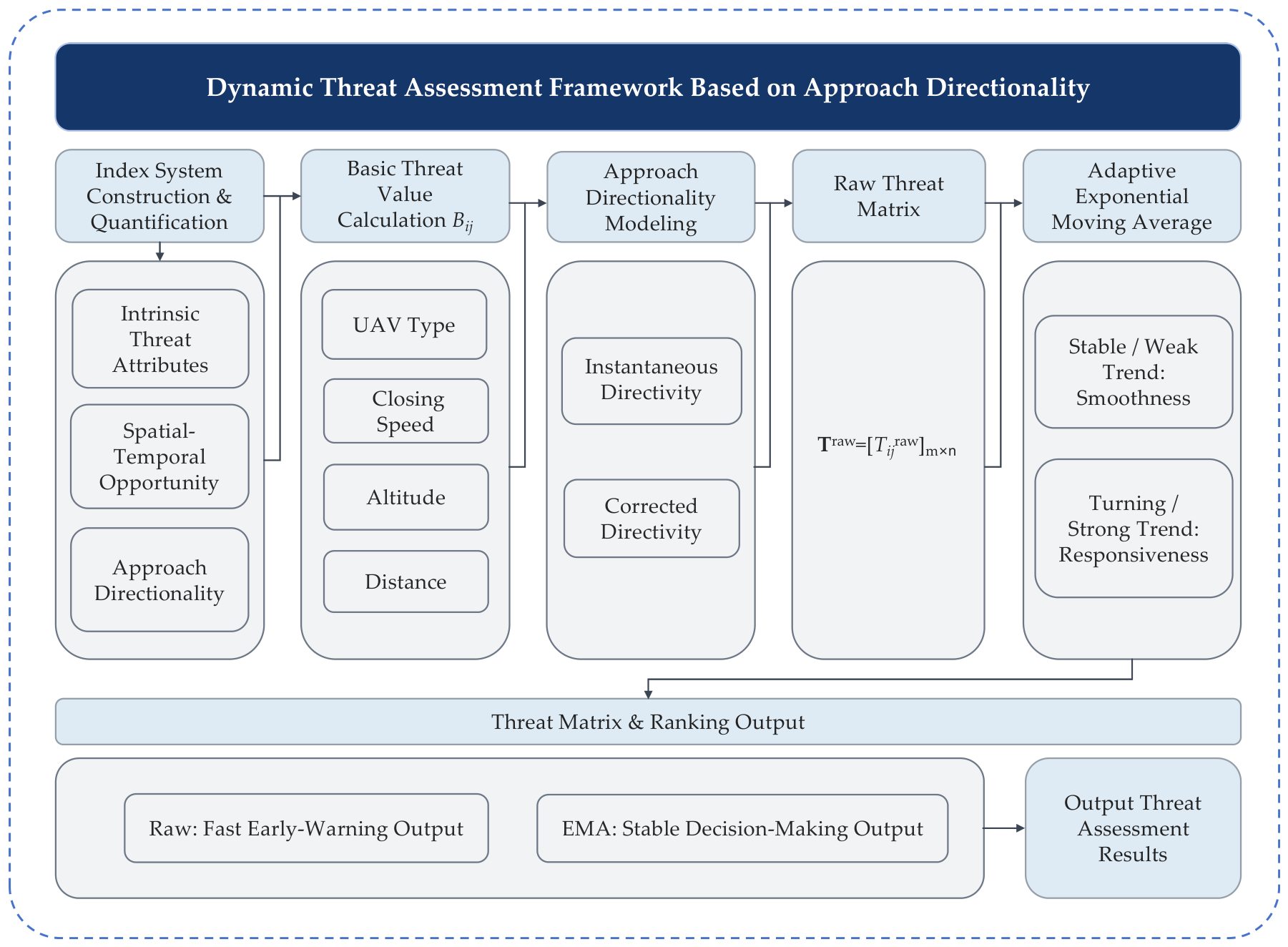
This section presents a three-dimensional approach-directionality-based dynamic threat assessment method for multi-UAV and multi-asset protection scenarios. The objective is to generate stable and responsive dynamic threat scores for all UAV–asset pairs over time, and to further construct the final threat matrix and threat rankings. Unlike conventional threat assessment methods that mainly rely on distance, speed, or static attributes, the proposed method jointly considers three-dimensional spatial proximity, velocity direction, attitude pointing, vertical approach tendency, and temporal ranking stability. The evaluation process of the proposed model is illustrated in Figure 2, and the overall threat assessment procedure is implemented through Algorithm 1.

Algorithm 1: Approach-Directionality-Based Dynamic Threat Assessment
Input: Multi-time UAV state data ${\{p_i(t),v_i(t),h_i(t),c_i\}}_{i=1}^m,$ $t\in \{1,2,\dots ,T\};$ positions of protected assets ${\left\{q_j\right\}}_{j=1}^n;$ parameter set $\mathsf{\Theta }=\{w_{\mathrm{type}},w_{\mathrm{speed}},w_{\mathrm{dist}},w_{\Delta h},w_z,\gamma ,{\omega }_b,K,\eta ,{\alpha }_{\min },{\alpha }_{\max },\lambda ,{\theta }_i(t),{\psi }_i(t),{\chi }_{ij}(t)\}.$
Output: instantaneous threat matrices $\{{\mathbf{T}}_{\mathrm{inst}}(t)\},$ trend-corrected threat matrices $\{{\tilde{\mathbf{T}}}_{\mathrm{inst}}(t)\},$ final dynamic threat matrices $\{\mathbf{S}(t)\},$ threat rankings $\{{\mathbf{\pi }}_i(t)\}.$
1:	Initialize $S_{ij}(0)=0$ for all UAV-asset pairs
2:	Initialize directionality history ${\mathcal{H}}_{ij}=\varnothing$ for all UAV-asset pairs
3:	for t = 1 to T do
4:	for i = 1 to m do
5:	for j = 1 to n do
6:	Compute ${\mathbf{r}}_{ij}(t)={\mathbf{q}}_i-{\mathbf{p}}_i(t)$
7:	Compute $d_{ij}(t)={‖{\mathbf{r}}_{ij}(t)‖}_2$
8:	Compute ${\mathbf{e}}_{ij}(t)={\displaystyle \frac{{\mathbf{r}}_{ij}(t)}{d_{ij}(t)+\epsilon }}$
9:	Compute basic threat $B_{ij}(t)$
10:	Compute velocity-based directionality $D_{v,ij}(t)$
11:	if attitude information is available then
12:	Compute body-axis vector ${\mathbf{b}}_{ij}(t)$
13:	Compute attitude-based directionality $D_{b,ij}(t)$
14:	else
15:	Set ${\omega }_b=0$
16:	end if
17:	Obtain reachability coefficient ${\chi }_{ij}(t)=0$
18:	Compute $D_{ij}(t)={\chi }_{ij}(t)[(1-{\omega }_b)D_{v,ij}(t)+{\omega }_b{D}_{b,ij}(t)]$
19:	Compute instantaneous threat $T_{\mathrm{inst},ij}(t)=B_{ij}(t)[1-\gamma +\gamma D_{ij}(t)]$
20:	Append $D_{ij}(t)$ to ${\mathcal{H}}_{ij}$ and keep the latest K samples
21:	Estimate trend slope $s_{ij}(t)$ from ${\mathcal{H}}_{ij}$
22:	Compute trend-corrected directionality ${\tilde{D}}_{ij}(t)=\mathrm{clip}\left(D_{ij}(t)(1+\eta s_{ij}(t)),0,1\right)$
23:	Compute trend-corrected threat ${\tilde{T}}_{ij}(t)=B_{ij}(t)\left[1-\gamma +\gamma {\tilde{D}}_{ij}(t)\right]$
24:	Compute adaptive smoothing factor ${\alpha }_{ij}(t)$
25:	if t = 1 then
26:	$S_{ij}(t)={\tilde{T}}_{ij}(t)$
27:	else
28:	$S_{ij}(t)={\alpha }_{ij}(t){\tilde{T}}_{ij}(t)+\left(1-{\alpha }_{ij}(t)\right)S_{ij}(t-1)$
29:	end if
30:	end for
31:	end for
32:	Form ${\mathbf{T}}_{\mathrm{inst}}(t)={\left[T_{\mathrm{inst},ij}(t)\right]}_{m\times n}$
33:	Form $\tilde{\mathbf{T}}(t)={\left[{\tilde{T}}_{ij}(t)\right]}_{m\times n}$
34:	Form final threat matrix $\mathbf{S}(t)={\left[S_{ij}(t)\right]}_{m\times n}$
35:	for j = 1 to n do
36:	Rank UAVs according to the j-th column of $S(t)$
37:	Store the ranking ${\mathbf{\pi }}_{ij}(t)$
38:	end for
39:	end for
40:	return $\left\{{\mathbf{T}}_{\mathrm{inst}}(t)\right\},\left\{\tilde{\mathbf{T}}(t)\right\},\left\{\mathbf{S}(t)\right\},\left\{{\mathbf{\pi }}_j(t)\right\}$

3.1. Problem Description

Consider a three-dimensional dynamic scenario consisting of mm UAVs and nn protected assets. The position and velocity of UAV ii at time tt are denoted as

$${\mathbf{p}}_i(t)={\left[x_i(t),y_i(t),z_i(t)\right]}^{\mathrm{T}}\in {\mathbb{R}}^3$$

(1)

$${\mathbf{v}}_i(t)={\left[v_i^x(t),v_i^y(t),v_i^z(t)\right]}^{\mathrm{T}}\in {\mathbb{R}}^3$$

(2)

The position of protected asset j is denoted as

$${\mathbf{q}}_i={\left[x_i,y_i,z_i\right]}^{\mathrm{T}}\in {\mathbb{R}}^3$$

(3)

The type threat coefficient of UAV i is represented by

$$c_i\in \left[0,1\right]$$

(4)

where a larger value indicates a higher platform capability, payload level, or high-priority.

The objective is to compute the final dynamic threat score of UAV i against protected asset j at each time step:

$$S_{ij}(t)\in \left[0,1\right]$$

(5)

The final dynamic threat scores of all UAV–asset pairs form the final threat matrix

$$\mathbf{S}(t)=\left[\begin{array}{cccc}{S}_{11}(t)& S_{12}(t)& \cdots & S_{1n}(t)\\ S_{21}(t)& S_{22}(t)& \cdots & S_{2n}(t)\\ ⋮& ⋮& \ddots & ⋮\\ S_{m1}(t)& S_{m2}(t)& \cdots & S_{mn}(t)\end{array}\right]\in {\mathbb{R}}^3$$

(6)

The j-th column of $\mathbf{S}(t)$ represents the threat distribution of all UAVs against protected asset j, while the i-th row represents the threat distribution of UAV i against all protected assets. For a given asset j, if

$$S_{aj}(t)>S_{bj}(t)$$

(7)

then UAV a is considered more threatening than UAV b to asset j at time t.

The relative position vector, distance, and line-of-sight unit vector from UAV i to asset j are defined as

$${\mathbf{r}}_{ij}(t)={\mathbf{q}}_j-{\mathbf{p}}_i(t)$$

(8)

$$d_{ij}(t)={‖{\mathbf{r}}_{ij}(t)‖}_2$$

(9)

$${\mathbf{e}}_{ij}(t)={\displaystyle \frac{{\mathbf{r}}_{ij}(t)}{d_{ij}(t)+\epsilon }}$$

(10)

where ε is a small positive constant used for numerical stability.

3.2. Three-Dimensional Basic Threat Modeling

The three-dimensional basic threat score describes the instantaneous threat level before temporal smoothing and ranking stabilization. Traditional 2D models typically use horizontal distance and ground speed. In realistic low-altitude airspace, however, UAVs may approach protected assets from different altitudes, fly below building tops, or descend into sheltered areas. Therefore, three-dimensional factors—altitude difference, vertical approach velocity, body-axis attitude, and terrain/obstacle constraints—are introduced to better characterize approach behavior in such environments.

The proposed three-dimensional basic threat score is defined as

$$B_{ij}(t)=w_{\mathrm{type}}{C}_i+w_{\mathrm{speed}}{C}_{ij}^{\mathrm{speed}}(t)+w_{\mathrm{dist}}{C}_{ij}^{\mathrm{dist}}(t)+w_{\Delta h}{C}_{ij}^{\Delta h}(t)+w_z{C}_{ij}^z(t)$$

(11)

where $B_{ij}(t)\in [0,1]$, and $w_{\mathrm{type}}$, $w_{\mathrm{speed}}$, $w_{\mathrm{dist}}$, $w_{\Delta h}$, and $w_z$ are the weights of the UAV type, 3D closing velocity, distance, altitude difference, and vertical approach factors, respectively. The weights satisfy

$$w_{\mathrm{type}}+w_{\mathrm{speed}}+w_{\mathrm{dist}}+w_{\Delta h}+w_z=1,w_{.}\ge 0$$

(12)

The type factor is

$$C_i=c_i$$

(13)

The three-dimensional closing velocity is computed as the projection of the UAV velocity onto the line-of-sight direction:

$$v_{ij}^{\mathrm{close}}(t)=\max \left(0,{\mathbf{v}}_i^{\mathrm{T}}(t){\mathbf{e}}_{ij}(t)\right)$$

(14)

The normalized closing-velocity factor is defined as

$$C_{ij}^{\mathrm{speed}}(t)=\tanh \left({\displaystyle \frac{v_{ij}^{\mathrm{close}}(t)}{v_{\mathrm{ref}}}}\right)$$

(15)

where $v_{\mathrm{ref}}$ is a reference velocity.

The distance factor is

$$C_{ij}^{\mathrm{close}}(t)=\exp \left(-{\displaystyle \frac{d_{ij}(t)}{r_{\mathrm{ref}}}}\right)$$

(16)

where $r_{\mathrm{ref}}$ is a reference distance.

The altitude difference is defined as

$$\Delta h_{ij}(t)=z_i(t)-z_j$$

(17)

The altitude proximity factor is

$$C_{ij}^{\Delta h}(t)=\exp \left(-{\displaystyle \frac{\left|\Delta h_{ij}(t)\right|}{h_{\mathrm{ref}}}}\right)$$

(18)

where $h_{\mathrm{ref}}$ is a reference altitude difference.

Since altitude difference alone cannot distinguish whether a UAV is approaching or moving away from the asset altitude, the vertical approach velocity is introduced as

$$v_{ij}^{z,\mathrm{app}}(t)=-sign\left(\Delta h_{ij}(t)\right)v_i^z(t)$$

(19)

If a UAV is above the asset and descending, then $v_{ij}^{z,\mathrm{app}}(t)>0$, indicating that it is approaching the asset altitude. The vertical approach factor is defined as

$$C_{ij}^z(t)=\sigma \left({\displaystyle \frac{v_{ij}^{z,\mathrm{app}}(t)}{v_z^{\mathrm{ref}}}}\right)$$

(20)

where

$$\sigma (x)={\displaystyle \frac{1}{1+\exp (-x)}}$$

(21)

is the sigmoid function, and $v_z^{\mathrm{ref}}$ is a reference vertical velocity.

3.3. Three-Dimensional Directionality Modeling and Instantaneous Threat Matrix

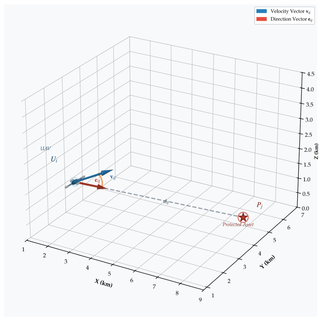
The basic threat score $B_{ij}(t)$ captures the three-dimensional spatial proximity between a UAV and an asset, but it does not fully capture whether the UAV exhibits a clear motion tendency toward the protected asset. In multi-asset scenarios, a UAV that is closer to an asset may not necessarily be directed toward it, whereas another UAV with a slightly larger distance but a stable heading toward the asset may pose a higher threat. Therefore, a directionality modulation mechanism is introduced, as shown in Figure 3.

The velocity-based directionality factor is defined as

$$D_{ij}^v(t)=\max \left(0,{\displaystyle \frac{{\mathbf{v}}_i^{\mathrm{T}}(t){\mathbf{e}}_{ij}(t)}{{‖{\mathbf{v}}_i(t)‖}_2+\epsilon }}\right)$$

(22)

where ε is a small positive constant for numerical stability. This factor is the non-negative part of the cosine similarity between the UAV velocity direction and the line-of-sight direction, i.e., $D_{ij}^{(v)}=\max (0,\cos \theta )$, where θ is the angle between the velocity vector and the line-of-sight vector. The $\max (0,\cdot )$ operation maps the cosine similarity from [−1, 1] to [0, 1], treating both laterally moving and receding UAVs as having no positive directional evidence of approach; their distinction remains partially represented by the signed closing-velocity factor in $B_{ij}(t)$. Although closing velocity and approach directionality are both derived from UAV motion geometry, they describe different aspects of threat: closing velocity measures the radial rate of range reduction, whereas directionality measures the angular alignment between velocity and asset-bearing vectors. Their separate encoding prevents over-emphasis on a single geometric feature and enables the model to distinguish, for example, a slowly approaching but well-aligned UAV from a fast UAV with only weak alignment. When the UAV speed falls below a prescribed threshold, the velocity direction becomes unreliable, and the directionality factor is down-weighted to a neutral value, as examined in the near-hovering case (Section 4.8). In 3D space, this factor captures both horizontal and vertical alignment: a UAV descending toward an asset may exhibit high directionality even at a large horizontal distance, which a 2D model would misjudge.

If attitude information is available, let ${\theta }_i(t)$ and ${\psi }_i(t)$ denote the pitch and yaw angles of UAV i, respectively. The body-axis unit vector is

$${\mathbf{b}}_i(t)={\left[\cos {\theta }_i(t)\cos {\psi }_i(t),\cos {\theta }_i(t)\sin {\psi }_i(t),\sin {\theta }_i(t)\right]}^{\mathrm{T}}$$

(23)

The attitude-based directionality factor is then

$$D_{ij}^b(t)=\max \left(0,{\mathbf{b}}_i^{\mathrm{T}}(t){\mathbf{e}}_{ij}(t)\right)$$

(24)

The velocity-based and attitude-based directionality factors are fused as

$$D_{ij}^{\mathrm{dir}}(t)=(1-{\omega }_b)D_{ij}^v(t)+{\omega }_b{D}_{ij}^b(t)$$

(25)

where ${\omega }_b\in [0,1]$ is the attitude fusion weight. If attitude information is unavailable, ${\omega }_b=0$.

In scenarios involving obstacles, terrain occlusion, or restricted areas, a reachability coefficient is introduced:

$${\chi }_{ij}(t)\in [0,1]$$

(26)

It describes the feasibility of the path from UAV i to asset j. In the present implementation, ${\chi }_{ij}(t)$ is defined as a simple binary visibility indicator: a ray is cast from the UAV to the protected asset, and ${\chi }_{ij}(t)=1$ if the direct line-of-sight is unobstructed, otherwise ${\chi }_{ij}={\chi }_{\min }$ with a default value of 0.5. This minimal model is adopted because more sophisticated reachability estimation (e.g., based on path planning or probabilistic obstacle maps) is beyond the scope of this work. The experimental ablation in Section 4.10 examines the effect of this basic reachability term, and ${\chi }_{ij}(t)$ is disabled by default in all other experiments. The integrated directionality factor is

$$D_{ij}(t)={\chi }_{ij}(t)D_{ij}^{\mathrm{dir}}(t)$$

(27)

If reachability constraints are not considered, ${\chi }_{ij}(t)=1$.

The directionality-modulated instantaneous threat score is defined as

$$T_{ij}^{\mathrm{inst}}(t)=B_{ij}(t)\left[1-\gamma +\gamma D_{ij}(t)\right]$$

(28)

where $\gamma \in [0,1]$ controls the strength of directionality modulation. When $\gamma =0$, the model degenerates into a non-directional basic threat model. As γ increases, directionality has a stronger influence on the threat score.

The multiplicative form in Equation (29) reflects the following design consideration. A UAV that is close to a protected asset and has a high basic threat value $B_{ij}$ may still pose a limited immediate threat if its motion direction is not aligned with the asset. Conversely, a UAV with a moderate $B_{ij}$ but a persistently high directionality toward the asset warrants greater attention. Therefore, $D_{ij}$ acts as a modulating term: when $D_{ij}$ is high, the basic threat factors are preserved and remain the primary discriminators among well-directed UAVs; when $D_{ij}$ is low, the overall threat score is appropriately attenuated. An additive combination would allow a UAV with a high basic threat but no directional alignment to retain a substantial portion of its score, which could lead to an overestimation of its immediate threat level. The modulation attenuates, rather than eliminates, the basic threat score when directional alignment is weak. The residual factor 1-γ prevents the model from assigning a zero threat to nearby UAVs whose direction estimates may be uncertain. Consequently, high basic threat and strong directional alignment are jointly favored in the final prioritization, without requiring either factor to be strictly necessary.

The instantaneous threat scores of all UAV–asset pairs form the instantaneous threat matrix:

$${\mathbf{T}}^{\mathrm{inst}}={\left[T_{ij}^{\mathrm{inst}}(t)\right]}_{m\times n}$$

(29)

It should be emphasized that ${\mathbf{T}}^{\mathrm{inst}}$ is not the final output matrix. It only represents the directionality-modulated threat estimate at the current time step. The final threat matrix is obtained after trend correction and adaptive smoothing.

3.4. Directionality Trend Correction

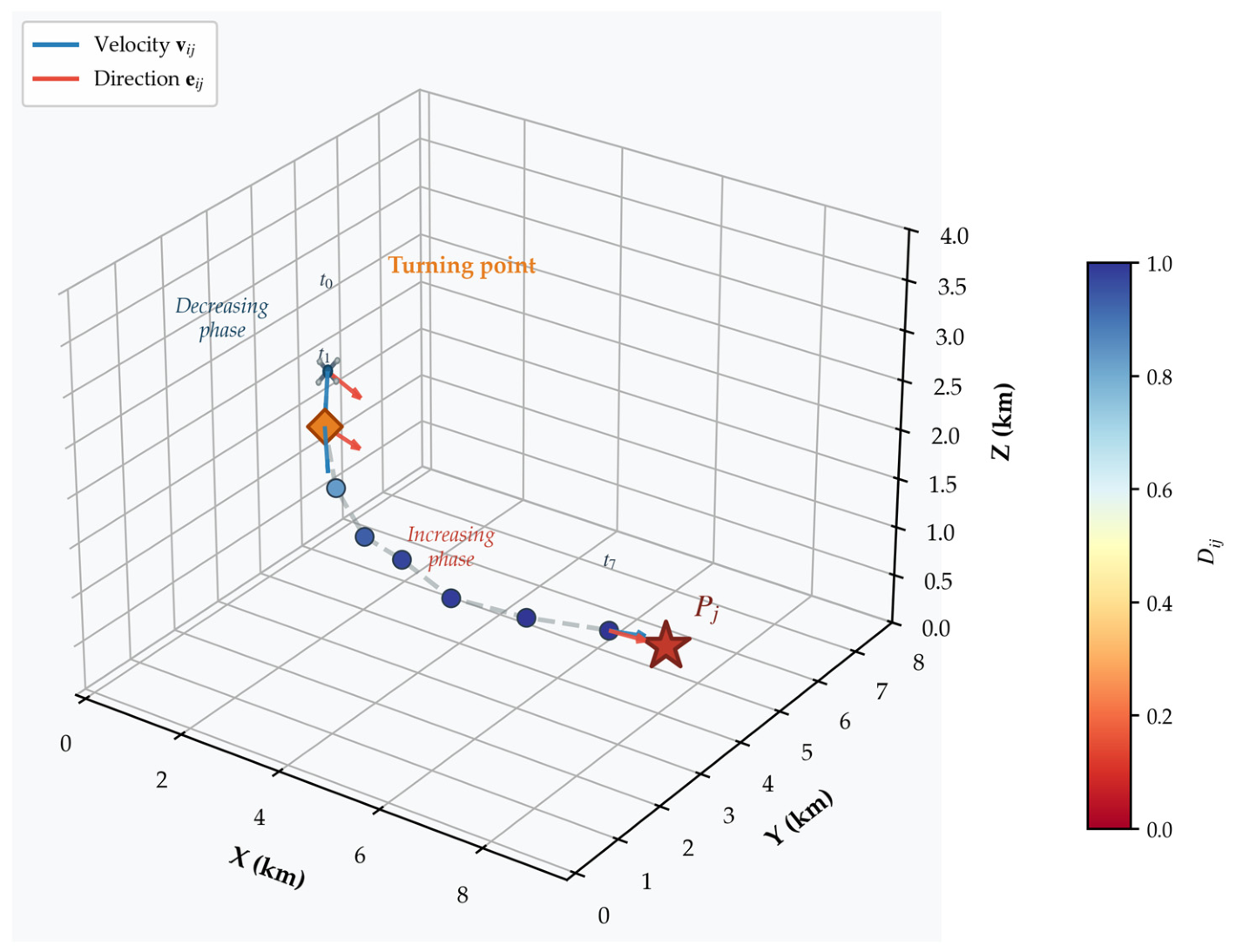
The instantaneous directionality $D_{ij}\left(t\right)$ may fluctuate due to measurement noise, short-term maneuvers, and attitude perturbations. Directly using ${\mathbf{T}}^{\mathrm{inst}}$ for ranking may cause frequent ranking changes between adjacent time steps. Conversely, overly strong smoothing may delay the response to genuine target switching. Therefore, a directionality trend correction mechanism is introduced, as illustrated in Figure 4.

For each UAV–asset pair (i,j), a directionality history window with a maximum length K is maintained:

$${\mathcal{H}}_{ij}\left(t\right)=\left\{D_{ij}\left(t-K+1\right),\dots ,D_{ij}\left(t\right)\right\}$$

(30)

If fewer than K historical samples are available, all available samples are used. Let the directionality sequence in the current window be

$$\left\{D_{ij}^{(1)},D_{ij}^{(2)},\dots D_{ij}^{(L)}\right\},L\le K$$

(31)

To quantify the temporal trend of directionality, the slope $s_{ij}(t)$ of the linear trend over the L points $(\mathcal{l},D_{ij}^{(\mathcal{l})})$ is estimated by ordinary least squares:

$$s_{ij}(t)={\displaystyle \frac{{\displaystyle {\sum }_{\mathcal{l}=1}^L(\mathcal{l}-\overline{\mathcal{l}})}(D_{ij}^{(\mathcal{l})}-{\overline{D}}_{ij})}{{{\displaystyle {\sum }_{\mathcal{l}=1}^L(\mathcal{l}-\overline{\mathcal{l}})}}^2+\epsilon }}$$

(32)

where

$$\overline{\mathcal{l}}={\displaystyle \frac{1}{L}}{\displaystyle {\displaystyle \sum _{\mathcal{l}=1}^L}\mathcal{l}},{\overline{D}}_{ij}={\displaystyle \frac{1}{L}}{\displaystyle {\displaystyle \sum _{\mathcal{l}=1}^L}{D}_{ij}^{(\mathcal{l})}}$$

(33)

A positive $s_{ij}\left(t\right)$ indicates that the directionality toward the asset is increasing, whereas a negative value indicates decreasing directionality.

The current directionality is corrected as

$${\tilde{D}}_{ij}(t)=\mathrm{clip}\left(D_{ij}\left(t\right)\left[1+\eta s_{ij}\left(t\right)\right],0,1\right)$$

(34)

where $\eta \ge 0$ is the trend correction gain, and $\mathrm{clip}(\cdot ,0,1)$ restricts the value to [0,1].

The trend-corrected instantaneous threat score is then

$${\tilde{T}}_{ij}(t)=B_{ij}(t)[1-\gamma +\gamma {\tilde{D}}_{ij}(t)]$$

(35)

The corresponding trend-corrected threat matrix is

$$\tilde{\mathbf{T}}(t)={\left[{\tilde{T}}_{ij}(t)\right]}_{m\times n}$$

(36)

Compared with ${\mathbf{T}}^{\mathrm{inst}}$, $\tilde{\mathbf{T}}(t)$ incorporates the local trend of directionality. It enhances responsiveness to persistent increases or decreases in approach directionality, thereby improving sensitivity to evolving approach tendencies. Because trend correction may also amplify local estimation noise, it does not by itself suppress short-term fluctuations. However, $\tilde{\mathbf{T}}(t)$ is still an instantaneous estimate and must be further processed to obtain the final dynamic threat matrix.

3.5. Adaptive Exponential Smoothing and Final Threat Matrix

To further improve temporal ranking stability, an adaptive exponential smoothing mechanism is used to update the final dynamic threat score. For each UAV–asset pair, the final score is computed as

$$S_{ij}(t)={\alpha }_{ij}(t){\tilde{T}}_{ij}(t)+\left[1-{\alpha }_{ij}(t)\right]S_{ij}(t-1)$$

(37)

Here, ${\tilde{T}}_{ij}(t)$ is the current trend-corrected instantaneous threat score, $S_{ij}(t-1)$ is the final threat score at the previous time step, and ${\alpha }_{ij}(t-1)\in \left[{\alpha }_{\min },{\alpha }_{\max }\right]$ is the adaptive smoothing coefficient.

The smoothing coefficient is adjusted according to the magnitude of the directionality trend:

$${\alpha }_{ij}(t)={\alpha }_{\min }+({\alpha }_{\max }-{\alpha }_{\min })\sigma \left(\lambda \left|s_{ij}(t)\right|\right)$$

(38)

where ${\alpha }_{\min }$ and ${\alpha }_{\max }$ are the lower and upper bounds of the smoothing coefficient, and λ controls the sensitivity to the trend slope.

When $\left|s_{ij}(t)\right|$ is small, the directionality is relatively stable, and a smaller ${\alpha }_{ij}(t)$ gives more weight to historical threat scores, thereby suppressing noise-induced fluctuations. When $\left|s_{ij}(t)\right|$ is large, the UAV may be forming a new approach trend or switching its target, and a larger ${\alpha }_{ij}(t)$ allows the model to respond more rapidly to current observations.

At the initial time step, the score can be initialized as

$$S_{ij}\left(0\right)={\tilde{T}}_{ij}(0)$$

(39)

Finally, the final dynamic threat scores of all UAV–asset pairs constitute the final threat matrix:

$$\mathbf{S}(t)={\left[S_{ij}(t)\right]}_{m\times n}=\left[\begin{array}{cccc}{S}_{11}(t)& S_{12}(t)& \cdots & S_{1n}(t)\\ S_{21}(t)& S_{22}(t)& \cdots & S_{2n}(t)\\ ⋮& ⋮& \ddots & ⋮\\ S_{m1}(t)& S_{m2}(t)& \cdots & S_{mn}(t)\end{array}\right]$$

(40)

Therefore, the final output of the proposed method is not the instantaneous threat matrix ${\mathbf{T}}^{\mathrm{inst}}(t)$, but the final dynamic threat matrix $S(t)$ after trend correction and adaptive smoothing. This matrix integrates spatial threat, directional intent, temporal trend, and dynamic stability, and serves as the basis for threat ranking and defensive resource allocation.

3.6. Threat Ranking and Stability Metrics

At each time step t, for protected asset j, all UAVs are ranked in descending order according to the j-th column of the final threat matrix $\mathbf{S}(t)$:

$${\mathbf{\pi }}_j(t)={\mathrm{argsort}}_i^{\downarrow }\left(S_{ij}(t)\right)$$

(41)

Here, ${\mathbf{\pi }}_j\left(t\right)$ denotes the threat ranking of all UAVs with respect to asset j. The top-ranked UAV is

$${\widehat{i}}_{1,j}(t)=\arg \underset{i}{\max }{S}_{ij}(t)$$

(42)

To evaluate temporal ranking stability, three metrics are used: Top-1 switching, Top-3 switching, and RankFluc.

Top-1 switching is defined as

$$\mathrm{S}{\mathrm{w}}_1={\displaystyle \sum _{j=1}^n{\displaystyle \sum _{t=2}^T\mathrm{II}\left[{\widehat{i}}_{1,j}(t)\ne {\widehat{i}}_{1,j}(t-1)\right]}}$$

(43)

where T is the number of time steps, and $\mathrm{II}\left[\cdot \right]$ is the indicator function. This metric measures how frequently the highest-threat UAV changes for each protected asset.

Let ${\mathcal{I}}_{3,j}(t)$ denote the set of the top three UAVs for asset j at time t. Top-3 switching is defined as

$$\mathrm{S}{\mathrm{w}}_3={\displaystyle \sum _{j=1}^n{\displaystyle \sum _{t=2}^T\mathrm{II}\left[{\mathcal{I}}_{3,j}(t)\ne {\mathcal{I}}_{3,j}(t-1)\right]}}$$

(44)

This metric evaluates the temporal stability of the high-threat candidate set.

The full-ranking fluctuation metric RankFluc is defined as

$$\mathrm{RankFluc}={\displaystyle \frac{1}{n\left(T-1\right)}}{\displaystyle \sum _{j=1}^n{\displaystyle \sum _{t=2}^T\left[1-{\rho }_s\left({\mathbf{\pi }}_j(t),{\mathbf{\pi }}_j(t-1)\right)\right]}}$$

(45)

where ${\rho }_s(\cdot ,\cdot )$ is the Spearman rank correlation coefficient. A smaller RankFluc indicates a more stable adjacent-time threat ranking.

It should be noted that ranking stability metrics should not be interpreted in isolation. Excessive smoothing, observation latency, or missed detections may reduce switching and RankFluc, but this does not necessarily indicate better threat identification. Therefore, these stability metrics are analyzed jointly with identification accuracy and response delay in the experiments.

4. Simulation Experiments and Result Analysis

4.1. Experimental Setup and Evaluation Metrics

4.1.1. Experimental Setup

To comprehensively evaluate the proposed three-dimensional modulated- directionality dynamic threat assessment method, we conduct experiments from several complementary perspectives: 3D vertical-approach discrimination, static identification performance, dynamic ranking stability, noise robustness, parameter sensitivity, practical observation degradation, representative difficult cases, computational efficiency, and 3D-factor ablation. The experiments are designed not only to examine whether the method can identify the most threatening UAV, but also to evaluate whether it can produce a stable, timely, and reliable threat ranking in dynamic multi-UAV scenarios.

Unless otherwise specified, the term proposed refers to the complete method described in Section 3, including 3D basic threat modeling, directionality modulation, directionality trend correction, and adaptive exponential smoothing. For the proposed method, all accuracy, delay, switching, and stability metrics are computed from the final dynamic threat matrix $\mathbf{S}(t)$, rather than from the instantaneous or intermediate trend-corrected threat matrix. This ensures that the evaluated output is consistent with the actual decision input produced by the method.

The following methods are compared in the experiments:

• NoDir: a model without directionality, using only the 3D basic threat factors;
• TOPSIS: a TOPSIS-based multi-attribute decision-making baseline, the detailed calculation procedure is provided in Appendix A;
• Inst: an instantaneous directionality model using the directionality-modulated instantaneous threat output;
• Raw: a trend-corrected model with directionality trend correction but without temporal smoothing;
• Fixed_EMA: an exponential smoothing model with a fixed smoothing coefficient;
• Sliding_Avg: a sliding-average smoothing model;
• Proposed: the complete proposed method, which outputs the final dynamic threat matrix $\mathbf{S}(t)$.

4.1.2. Evaluation Metrics

The main evaluation metrics include identification accuracy, response delay, and several ranking stability measures. TransferAcc measures the proportion of UAVs whose predicted high-threat asset matches the ground-truth target, directly capturing the method’s threat-object association capability. Detection delay quantifies the time required for a method to stably identify the new threat target after a true threat transfer, reflecting responsiveness for timely situational awareness. Dynamic Top-1 accuracy evaluates whether the highest-threat UAV identified by the method matches the ground-truth at each time step throughout the dynamic scenario.

Top-1 switching and Top-3 switching quantify the temporal variation in the top-ranked UAV and the high-threat candidate set, respectively; lower switching counts—when achieved without sacrificing accuracy or delay—indicate more actionable threat rankings that reduce resource reallocation oscillations. Fluc measures the temporal fluctuation of individual threat scores, while RankFluc evaluates the stability of the complete threat ranking via Spearman correlation between adjacent time steps; these metrics capture finer-grained stability characteristics complementing the switching measures.

The Spearman rank correlation is used for pairwise ranking consistency evaluation between methods. Collectively, these metrics cover three essential aspects of dynamic threat assessment: correctness, timeliness, and stability. It should be noted that stability metrics should be interpreted jointly with accuracy and delay: stale or missing observations may artificially reduce temporal fluctuation, and therefore a lower Fluc or fewer switches alone do not necessarily indicate better threat assessment.

4.2. Three-Dimensional Vertical-Approach Discrimination

4.2.1. Purpose and Experimental Setup

A key difference between low-altitude UAV threat assessment and conventional two-dimensional target ranking is that altitude difference and vertical motion can substantially affect threat judgment. A model relying only on horizontal distance or horizontal velocity may incorrectly assign a higher threat level to a UAV that is horizontally closer but moving away from the protected asset in altitude, while underestimating another UAV that is horizontally farther but descending toward the asset.

To verify the necessity of 3D modeling, a representative vertical-approach scenario is constructed. The scenario contains two UAVs and one protected asset. UAV-0 is horizontally closer to the asset but moves vertically away from the asset altitude, whereas UAV-1 is horizontally farther but descends toward the asset altitude. The 3D model explicitly accounts for altitude difference and vertical motion, so it correctly identifies UAV-1 as the high-threat object despite its longer horizontal distance, because the descending motion indicates an approaching tendency that cannot be captured by horizontal metrics alone. Therefore, UAV-1 is defined as the ground-truth high-threat UAV.

To avoid confounding the contribution of 3D factors with that of the complete dynamic stabilization mechanism, three variants are compared: 2D_No_Vertical, 3D_Base, and 3D_Proposed. The 2D_No_Vertical variant ignores altitude difference and vertical-approach information. The 3D_Base variant incorporates 3D altitude and vertical-approach factors but does not include the complete dynamic stabilization pipeline. The 3D_Proposed variant corresponds to the complete proposed method. This setting allows the contribution of 3D modeling and the additional effect of dynamic stabilization to be examined separately.

4.2.2. Results and Analysis

As shown in

Table 2. Results of 3D vertical-approach discrimination.

Method	Top-Threat Accuracy	First Sustained Correct Time Step	Mean Score Gap of True High-Threat UAV
2D_No_Vertical	0.433	35	−0.0008
3D_Base	1.000	0	+0.1485
3D_Proposed	1.000	0	+0.1470

, 2D_No_Vertical achieves a top-threat accuracy of only 0.433 and does not reach sustained correct identification until time step 35. Its mean score gap for the true high-threat UAV is slightly negative, indicating that the 2D model tends to favor UAV-0 because of its shorter horizontal distance, even though UAV-1 is the truly more threatening UAV in 3D space.

In contrast, 3D_Base correctly identifies UAV-1 from the beginning of the sequence, achieving an accuracy of 1.000 and a clear positive score gap. This result demonstrates that altitude difference and vertical-approach motion are not merely auxiliary features, but essential factors in low-altitude 3D threat assessment.

The performance of 3D_Proposed is very close to that of 3D_Base, indicating that in this representative scenario, the main improvement comes from 3D modeling itself, while the complete dynamic stabilization mechanism does not weaken 3D discrimination capability. This experiment confirms that ignoring the vertical dimension may lead to an incorrect prioritization of horizontally closer but actually less threatening UAVs.

4.3. Static Monte Carlo Identification Performance

4.3.1. Purpose and Experimental Setup

The static Monte Carlo experiment evaluates the basic identification capability of different methods in randomized 3D multi-UAV scenarios. In each trial, UAV positions, velocities, type scores, and protected asset locations are randomly generated, and identification accuracy is evaluated according to the ground-truth high-threat object. A total of 200 independent trials is conducted.

It should be noted that the static experiment is not based on a completely isolated single-frame input. Instead, the final state of a short quasi-static trajectory is used for evaluation, so the historical update process of the proposed method remains well defined. The purpose of this experiment is not to demonstrate the advantage of dynamic smoothing, but to verify whether the complete method introduces any significant loss in basic identification ability. The dynamic stability advantage is further analyzed in Section 4.4.

4.3.2. Results and Analysis

As reported in

Table 3. Results of the static Monte Carlo experiment.

Method	Identification Accuracy
NoDir	0.555 ± 0.234
TOPSIS	0.560 ± 0.232
Inst	0.685 ± 0.206
Proposed	0.679 ± 0.207

, NoDir and TOPSIS obtain accuracies of 0.555 and 0.560, respectively, showing comparable performance. This indicates that threat judgment based only on type, distance, speed magnitude, and altitude-related factors is still insufficient for identifying the actual threat intent of UAVs.

After introducing directionality modulation, Inst improves the accuracy to 0.685, substantially outperforming the NoDir and TOPSIS baselines. This demonstrates that whether a UAV is moving toward a protected asset is a key indicator of threat level. Threat assessment should therefore consider not only how close or fast a UAV is, but also whether its motion direction is aligned with the protected asset.

The Proposed method achieves an accuracy of 0.679, only slightly lower than Inst. This is expected because the output of the proposed method is temporally stabilized and thus slightly less sensitive to instantaneous changes. Nevertheless, the small difference indicates that the adaptive smoothing mechanism does not introduce a notable loss in basic identification capability.

4.4. Dynamic Monte Carlo Ranking Stability

4.4.1. Purpose and Experimental Setup

The central challenge in dynamic threat assessment is that the true high-threat object may change over time, while short-term maneuvers, direction perturbations, and observation noise can cause frequent threat-ranking fluctuations. An ideal method should therefore satisfy two requirements simultaneously: it should respond promptly to true threat switches and suppress unnecessary ranking changes induced by transient disturbances.

To evaluate this capability, a dynamic Monte Carlo experiment is conducted. In each trial, continuous 3D multi-UAV trajectories are generated, and a target-switching process is embedded in the trajectories. All methods are evaluated on the same trajectories in a paired manner to reduce the influence of random scenario variation. A total of 200 trials are performed, and accuracy, response delay, Top-1 switching, Top-3 switching, Fluc, RankFluc, and Spearman rank consistency are evaluated.

For fairness, each method is evaluated using its own final output. Specifically, Inst uses the instantaneous directionality-modulated output, Raw uses the trend-corrected output, Fixed_EMA and Sliding_Avg use their respective smoothed outputs, and Proposed uses the final dynamic threat matrix $\mathbf{S}(t)$.

4.4.2. Results and Analysis

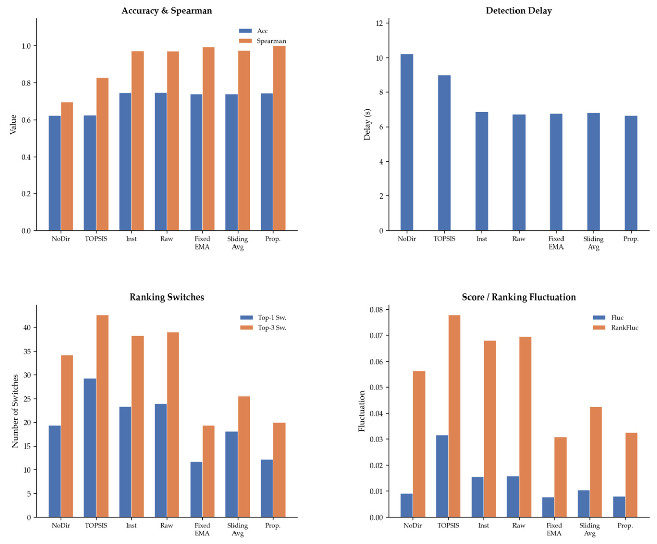
Figure 5 presents the overall performance of all methods across the seven metrics. The detailed numerical results are reported in

Table 4. Results of dynamic Monte Carlo experiments.

Method	Acc	Delay (s)	Top-1 Sw.	Top-3 Sw.	Fluc	RankFluc	Spearman
NoDir	0.623	10.23	19.32	34.18	0.0090	0.0562	0.697
TOPSIS	0.625	8.99	29.21	42.60	0.0315	0.0778	0.828
Inst	0.745	6.88	23.34	38.22	0.0155	0.0679	0.974
Raw	0.746	6.73	23.93	38.93	0.0158	0.0694	0.973
Fixed_EMA	0.738	6.78	11.71	19.34	0.0078	0.0308	0.993
Sliding_Avg	0.738	6.82	18.04	25.55	0.0103	0.0425	0.977
Proposed	0.743	6.65	12.19	19.93	0.0081	0.0325	1.000

. As shown, NoDir and TOPSIS achieve accuracies of 0.623 and 0.625, respectively, which are substantially lower than those of the directionality-based methods. This again confirms the importance of directionality information in dynamic threat identification. In particular, although NoDir does not produce the highest switching count, its response delay reaches 10.23, indicating that its apparently moderate switching behavior is mainly due to insufficient responsiveness rather than effective stabilization.

The Inst method achieves an accuracy of 0.745, demonstrating that instantaneous directionality modulation is effective for improving dynamic identification. However, its Top-1 switching, Top-3 switching, Fluc, and RankFluc remain relatively high, indicating that the ranking is sensitive to short-term direction perturbations. The Raw method performs similarly to Inst in terms of accuracy and delay, but its stability metrics do not improve and are even slightly worse. This suggests that trend correction alone is insufficient for suppressing ranking fluctuations; without temporal smoothing, local variations in directionality may still be retained or even amplified.

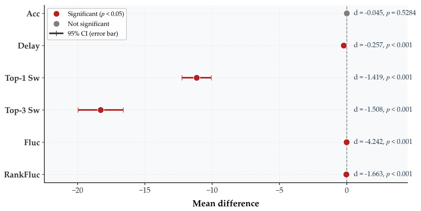
By contrast, the proposed method substantially improves dynamic stability with almost no loss of accuracy. Its accuracy is 0.743, very close to the 0.745 of Inst, and the paired comparison in

Table 5. Paired statistical comparison between Proposed and Inst.

Metric	Mean Difference	95% CI	Cohen’s d	p-Value
Acc	−0.0020	(−0.0082, +0.0042)	−0.045	0.5284
Delay	−0.2290	(−0.3523, −0.1057)	−0.257	0.0003
Top-1 Sw	−11.1500	(−12.2391, −10.0609)	−1.419	<0.0001
Top-3 Sw	−18.2850	(−19.9660, −16.6040)	−1.508	<0.0001
Fluc	−0.0074	(−0.0076, −0.0071)	−4.242	<0.0001
RankFluc	−0.0354	(−0.0384, −0.0325)	−1.663	<0.0001

shows that the accuracy difference is not statistically significant. Two-sided paired t-tests were applied to the trial-wise paired differences between the proposed method and Inst. Given the relatively large number of paired trials (200), the tests are expected to be reasonably robust to moderate deviations from normality [40]. Figure 6 provides a forest-plot visualization of the paired differences with 95% confidence intervals and Cohen’s d, where significant improvements are highlighted in red. Meanwhile, compared with Inst, the proposed method reduces Top-1 switching by approximately 47.8%, Top-3 switching by approximately 47.9%, Fluc by approximately 47.7%, and RankFluc by approximately 52.1%. All these improvements are statistically significant (Table 5). Given that all unadjusted p-values are well below 0.001, none of the significant differences would be altered by Bonferroni correction. In contrast, Raw shows no improvement in stability metrics compared with Inst, confirming that trend correction alone is insufficient for achieving ranking stability.

It is worth noting that Fixed_EMA yields slightly lower Top-1 switching, Top-3 switching, and RankFluc than the proposed method, while the proposed method achieves marginally higher accuracy and a shorter mean response delay. These complementary differences suggest that Fixed_EMA and the proposed method represent different operating points along the stability–responsiveness trade-off: Fixed_EMA prioritizes ranking stability at the cost of slightly delayed response, whereas the proposed method, through adaptive smoothing, aims to maintain responsiveness while still achieving substantial stability improvements over Inst and Raw.

The pairwise Spearman analysis in Table 4 measures the rank correlation between each method’s output ranking and the final threat ranking produced by the proposed method; consequently, the proposed method’s Spearman equals one by definition and is not an independent performance indicator. Among the compared methods, Fixed_EMA produces rankings most similar to those of the proposed method, indicating that the two share a consistent view of the overall threat landscape despite their differing stability–responsiveness trade-offs. This similarity is relevant in practical defense systems because resource allocation often depends not only on the top-ranked UAV but also on the stability of a high-threat candidate set such as the Top-3 list.

4.5. Noise Robustness Analysis

4.5.1. Purpose and Experimental Setup

To evaluate robustness to observation noise, zero-mean Gaussian noise is added to UAV position observations at four standard deviation levels: 1 m, 3 m, 6 m, and 10 m. All noise levels share the same set of 100 underlying trajectories, and for each trajectory, Inst, Raw, and Proposed are evaluated using identical noise realizations at each level. This paired design ensures that differences among methods are attributable to the methods themselves rather than to scenario or noise variation. The Inst method reflects the noise sensitivity of instantaneous directionality modeling, Raw examines whether trend correction alone improves noise robustness, and Proposed evaluates the combined effect of trend correction and adaptive smoothing, thereby explicitly separating the contributions of different modules.

4.5.2. Results and Analysis

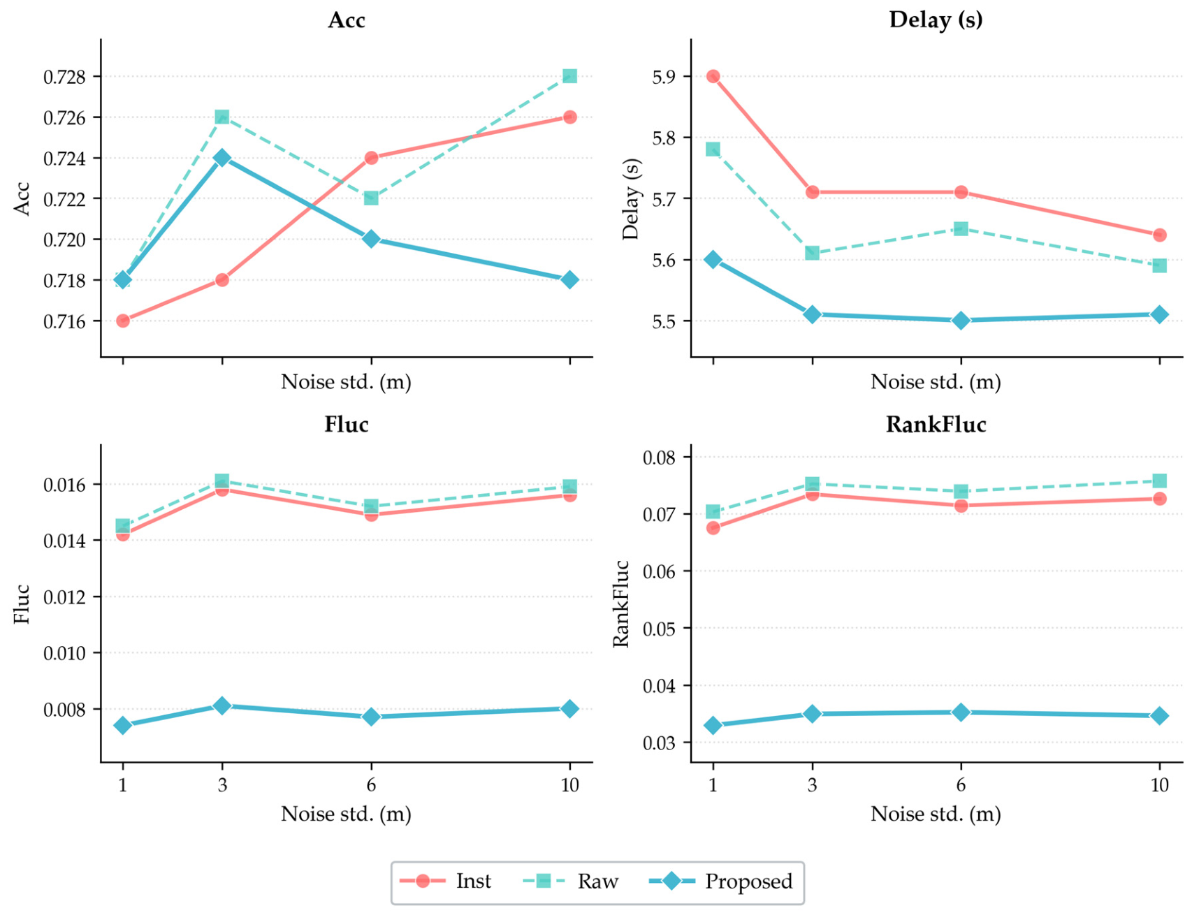
As shown in

Table 6. Performance of Inst, Raw, and Proposed under different noise levels.

Noise Std./m	Method	Acc	Delay (s)	Fluc	RankFluc
1.0	Inst	0.716	5.90	0.0142	0.0675
1.0	Raw	0.718	5.78	0.0145	0.0703
1.0	Proposed	0.718	5.60	0.0074	0.0329
3.0	Inst	0.718	5.71	0.0158	0.0734
3.0	Raw	0.726	5.61	0.0161	0.0752
3.0	Proposed	0.724	5.51	0.0081	0.0349
6.0	Inst	0.724	5.71	0.0149	0.0714
6.0	Raw	0.722	5.65	0.0152	0.0739
6.0	Proposed	0.720	5.50	0.0077	0.0352
10.0	Inst	0.726	5.64	0.0156	0.0726
10.0	Raw	0.728	5.59	0.0159	0.0757
10.0	Proposed	0.718	5.51	0.0080	0.0346

and visualized in Figure 7, the proposed method consistently achieves substantially lower Fluc and RankFluc than both Inst and Raw across all tested noise levels. Even when the noise standard deviation increases to 10 m, the proposed method reduces Fluc from 0.0156 to 0.0080 and RankFluc from 0.0726 to 0.0346 compared with Inst, corresponding to reductions of approximately 48.7% and 52.3%, respectively. Comparable reductions are observed at the lower noise levels. These results demonstrate that the final dynamic threat matrix effectively suppresses noise-induced score fluctuations and ranking variations, thereby improving the temporal stability of threat assessment under noisy observations.

Table 7. Main paired statistical differences in the noise robustness experiment.

Noise Std./m	Comparison	ΔAcc	ΔDelay (s)	ΔFluc	ΔRankFluc
1.0	Proposed—Inst	+0.0020	−0.3000	−0.0068	−0.0346
1.0	Proposed—Raw	0.0000	−0.1740	−0.0071	−0.0374
1.0	Raw—Inst	+0.0020	−0.1260	+0.0003	+0.0028
3.0	Proposed—Inst	+0.0060	−0.2020	−0.0076	−0.0386
3.0	Proposed—Raw	−0.0020	−0.1000	−0.0079	−0.0403
3.0	Raw—Inst	+0.0080	−0.1020	+0.0003	+0.0017
6.0	Proposed—Inst	−0.0040	−0.2040	−0.0073	−0.0362
6.0	Proposed—Raw	−0.0020	−0.1520	−0.0076	−0.0387
6.0	Raw—Inst	−0.0020	−0.0520	+0.0003	+0.0025
10.0	Proposed—Inst	−0.0080	−0.1280	−0.0076	−0.0380
10.0	Proposed—Raw	−0.0100	−0.0760	−0.0079	−0.0411
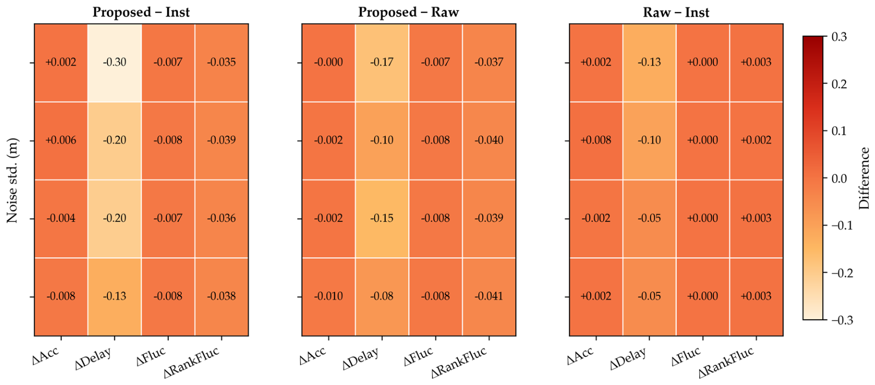
10.0	Raw—Inst	+0.0020	−0.0520	+0.0003	+0.0031

and Figure 8 further clarify the contributions of different modules. The Raw method, which includes directionality trend correction but does not apply final adaptive smoothing, slightly increases Fluc and RankFluc compared with Inst in most cases. This indicates that trend correction alone may enhance the responsiveness to directional changes, but it may also amplify local perturbations in directionality estimation when the observations are noisy. In contrast, the proposed method consistently yields the lowest Fluc and RankFluc, confirming that the adaptive EMA smoothing mechanism is the key component responsible for stable output generation.

In terms of identification accuracy, the proposed method maintains a comparable level of performance to Inst and Raw across different noise intensities. The accuracy values remain within a narrow range, indicating that the smoothing mechanism does not substantially degrade high-threat identification. Nevertheless, under the 10 m noise condition, the proposed method shows a slight accuracy decrease compared with Raw. This result reflects the inherent trade-off between instantaneous sensitivity and temporal stability: under strong observation noise, smoothing can suppress not only random perturbations but also some short-term variations that may be useful for instantaneous identification.

Overall, the noise robustness experiment demonstrates that the proposed method substantially improves the stability of dynamic threat assessment while maintaining competitive identification accuracy. The comparison with Raw further shows that directionality trend correction improves dynamic responsiveness but is insufficient to ensure noise robustness by itself, whereas adaptive smoothing plays a decisive role in reducing score fluctuations and ranking switches. Therefore, the proposed method is particularly suitable for safety monitoring applications in which stable and reliable threat ranking is more important than highly sensitive but unstable instantaneous decisions.

4.6. Parameter Sensitivity Analysis

4.6.1. Purpose and Experimental Setup

The proposed method contains several key parameters, including the directionality history length, directionality modulation weight, trend-correction gain, and maximum smoothing coefficient. The parameter sensitivity experiment investigates whether the performance of the method depends on fine-tuning and identifies which parameters have the most significant influence.

Eighty shared random scenarios are generated. For each experiment, only one parameter is varied while all other parameters are fixed at their default values. Identification accuracy and response delay are used as the main evaluation metrics to analyze the influence of parameter changes on recognition capability and dynamic responsiveness.

4.6.2. Results and Analysis

Table 8. Results of parameter sensitivity analysis.

Parameter	Value	Acc	Delay (s)
K	4	0.703 ± 0.212	5.79
K	6	0.707 ± 0.212	5.80
K	8	0.707 ± 0.214	5.74
K	10	0.705 ± 0.212	5.80
K	12	0.707 ± 0.210	5.82
K	16	0.703 ± 0.214	5.87
γ	0.3	0.662 ± 0.234	6.83
γ	0.5	0.690 ± 0.210	6.15
γ	0.6	0.705 ± 0.212	5.80
γ	0.7	0.722 ± 0.213	5.53
γ	0.9	0.740 ± 0.213	5.00
η	0.5	0.705 ± 0.212	5.95
η	1.0	0.702 ± 0.210	5.94
η	1.5	0.705 ± 0.212	5.89
η	2.0	0.705 ± 0.212	5.80
η	3.0	0.707 ± 0.214	5.71
αmax	0.5	0.702 ± 0.207	5.94
αmax	0.6	0.703 ± 0.214	5.89
αmax	0.7	0.703 ± 0.214	5.83
αmax	0.85	0.705 ± 0.212	5.80
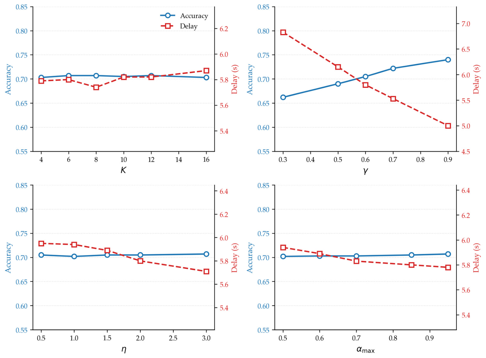
αmax	0.95	0.707 ± 0.210	5.78

and Figure 9 show that the method is not sensitive to the history length K. When K varies from 4 to 16, both accuracy and delay remain within a narrow range. This indicates that directionality trend estimation mainly relies on local temporal information and does not require an excessively long history. A very long window may even introduce outdated states and slightly weaken dynamic responsiveness.

The directionality modulation weight γ has the most pronounced effect. As γ increases from 0.3 to 0.9, the accuracy improves, and the response delay decreases. This suggests that, in the simulated scenarios, directionality provides strong discriminative information for identifying the true threat. Whether a UAV is moving toward a protected asset is therefore a critical factor for distinguishing real approach behavior from non-threatening proximity.

The trend-correction gain η and the maximum smoothing coefficient α_max have relatively moderate effects. Increasing η slightly reduces the response delay, indicating that trend information helps the model react to persistent approach behavior. A larger α_max also slightly reduces delay, because a higher update coefficient allows the smoothed output to follow changes more quickly.

Overall, the sensitivity of the method to the history length K, the trend-correction gain η, and the maximum smoothing coefficient αmax is relatively low, indicating that the reported performance does not rely on fine-tuning these parameters. The directionality modulation weight γ has a more pronounced influence, which is expected because it directly controls the relative importance of directionality information. A larger γ should not be interpreted as universally optimal: although a higher directionality weight improves performance in the current simulation environment, it may amplify direction-estimation errors under strong noise, low-speed hovering, abrupt maneuvers, or inaccurate velocity measurements. The default parameters are therefore selected to balance identification performance, noise robustness, and cross-scenario generalization, rather than to maximize a single metric in one experiment.

4.7. Practical Observation Degradation

4.7.1. Purpose and Experimental Setup

In practical deployment scenarios, the threat assessment model may receive sensor data that deviates from ground-truth states due to factors such as communication latency, missed detections, clutter, and suboptimal filtering. To systematically evaluate the method’s response under such non-ideal conditions, four types of observation imperfections are considered: observation latency, missed detection, clutter, and Kalman filtering. Observation latency means that the model receives delayed UAV states. Missed detection means that the current observation is unavailable at some time steps, and the last valid observation is reused. Clutter introduces erroneous perturbations into the observed state. Kalman filtering first smooths the observed trajectory using a constant-velocity model and then feeds the filtered state into the threat assessment method. Each degradation type is synthetically injected at multiple severity levels into the simulated observations, allowing both the relative robustness (Proposed vs. Inst) and the absolute sensitivity (Proposed relative to its own ideal-observation baseline) to be quantified. It should be noted that this experiment uses parameterized synthetic degradations rather than recorded sensor tracks from operational deployments; validation using measured sensor data remains an important future direction.

4.7.2. Results and Analysis

Table 9. Performance of Inst and Proposed under practical observation degradation.

Condition	Method	Acc	Delay (s)	Fluc
baseline	Inst	0.715	5.93	0.0154
baseline	Proposed	0.733	5.61	0.0079
latency = 2	Inst	0.707	6.09	0.0149
latency = 2	Proposed	0.718	5.74	0.0076
latency = 5	Inst	0.705	6.17	0.0140
latency = 5	Proposed	0.698	6.00	0.0072
miss = 15%	Inst	0.718	5.81	0.0135
miss = 15%	Proposed	0.730	5.63	0.0075
miss = 30%	Inst	0.713	5.68	0.0114
miss = 30%	Proposed	0.718	5.58	0.0071
clutter = 10%	Inst	0.700	6.01	0.0231
clutter = 10%	Proposed	0.715	5.65	0.0114
clutter = 25%	Inst	0.715	6.14	0.0341
clutter = 25%	Proposed	0.718	5.56	0.0163
KF	Inst	0.725	5.61	0.0129
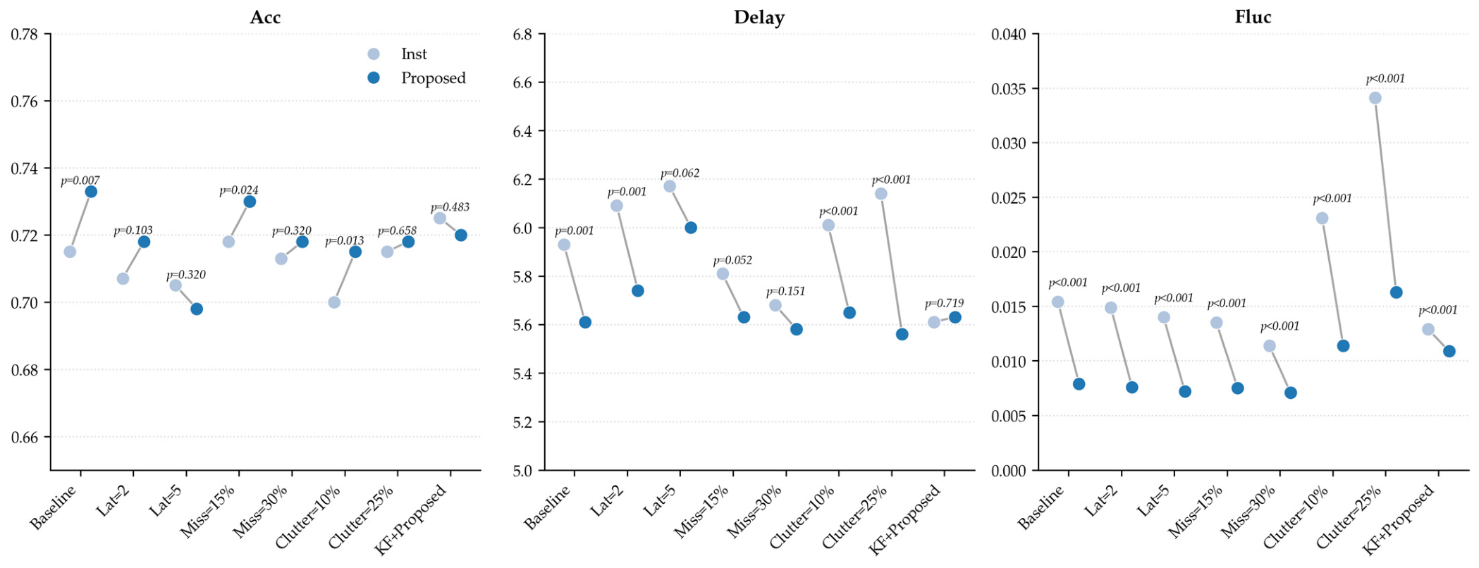
KF	Proposed	0.720	5.63	0.0109

and

Table 10. Paired differences between Proposed and Inst.

Condition	ΔAcc	p (Acc)	ΔDelay (s)	p (Delay)	ΔFluc	p (Fluc)
baseline	+0.0175	0.0073	−0.3225	0.0013	−0.0075	<0.0001
latency = 2	+0.0100	0.1028	−0.3525	0.0011	−0.0072	<0.0001
latency = 5	−0.0075	0.3204	−0.1650	0.0621	−0.0068	<0.0001
miss = 15%	+0.0125	0.0244	−0.1800	0.0520	−0.0059	<0.0001
miss = 30%	+0.0050	0.3204	−0.1025	0.1511	−0.0043	<0.0001
clutter = 10%	+0.0150	0.0134	−0.3575	0.0002	−0.0117	<0.0001
clutter = 25%	+0.0025	0.6576	−0.5825	<0.0001	−0.0178	<0.0001
KF	−0.0050	0.4830	+0.0175	0.7187	−0.0021	<0.0001

and Figure 10 show that, under most practical degradation conditions, the proposed method achieves lower Fluc than Inst and usually yields a lower response delay. This indicates that the complete dynamic stabilization pipeline remains effective under non-ideal inputs such as latency, missed detections, and clutter.

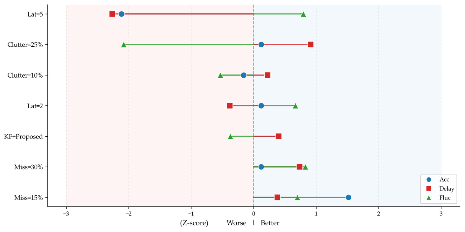
Under the baseline condition, the proposed method improves accuracy by 0.0175, reduces response delay by 0.3225, and reduces Fluc by 0.0075 compared with Inst. Under the latency = 2 condition, it still maintains a lower delay and significantly lower Fluc. However, when the latency increases to five time steps, the accuracy of the proposed method becomes slightly lower than that of Inst, although the difference is not statistically significant.

Table 11. Changes in Proposed relative to its own baseline.

Condition	ΔAcc	p (Acc)	ΔDelay (s)	p (Delay)	ΔFluc	p (Fluc)
latency = 2	−0.0150	0.0330	+0.1275	0.0843	−0.0003	<0.0001
latency = 5	−0.0350	0.0036	+0.3925	0.0045	−0.0007	<0.0001
miss = 15%	−0.0025	0.3204	+0.0200	0.2791	−0.0004	<0.0001
miss = 30%	−0.0150	0.0134	−0.0300	0.4133	−0.0008	<0.0001
clutter = 10%	−0.0175	0.0073	+0.0425	0.5819	+0.0035	<0.0001
clutter = 25%	−0.0150	0.0330	−0.0550	0.6221	+0.0084	<0.0001
KF	−0.0125	0.0958	+0.0175	0.8316	+0.0030	<0.0001

and Figure 11 further show that latency is the most detrimental factor for the proposed method itself: under latency = 5, accuracy drops by 0.0350 and delay increases by 0.3925 relative to its own baseline (both p < 0.01). This suggests that stale observations can weaken the effectiveness of trend estimation and adaptive updating, especially when true threat switches occur.

Missed detections have a comparatively mild effect on the proposed method. At a 15% miss rate, the changes in accuracy and delay are not statistically significant, whereas the small reduction in Fluc is statistically significant (Table 11). The corresponding markers in Figure 11 cluster near the zero baseline, indicating that the temporal stabilization mechanism can tolerate occasional missing observations. At a 30% miss rate, the accuracy advantage diminishes, but the stability advantage remains evident. It should be noted that missed detections cause the last valid observation to be reused; therefore, a reduction in Fluc does not necessarily imply more accurate situational estimation. It may partly reflect artificially slowed input variation. For this reason, missed-detection results should always be interpreted together with accuracy and delay.

Under clutter conditions, Inst is strongly affected by erroneous perturbations. Its Fluc increases to 0.0341 under clutter = 25%, whereas the proposed method reduces it to 0.0163. Table 11 confirms that clutter primarily increases score fluctuation, while also causing a modest but statistically significant reduction in accuracy. This demonstrates that the proposed method is more robust to clutter-induced disturbances. Although the accuracy advantage under clutter = 25% is not significant, the proposed method provides a substantially more stable and faster threat output, which is desirable for downstream defense decision-making.

Under the Kalman-filtered condition, the proposed method does not clearly outperform Inst, and its Fluc increases relative to its own baseline. Table 11 shows that Kalman filtering produces no statistically significant change in accuracy or delay, while the increase in Fluc relative to the proposed method’s baseline is statistically significant. This indicates that simple constant-velocity Kalman filtering does not necessarily improve threat assessment. Threat assessment requires not only smooth position trajectories but also timely recognition of directionality changes and threat switches. A constant-velocity filter may introduce lag for maneuvering UAVs. More advanced maneuver-aware filtering and outlier rejection mechanisms should therefore be considered in practical applications.

4.8. Representative Difficult Cases and Failure-Case Analysis

4.8.1. Purpose and Experimental Setup

To analyze the applicability boundaries of the proposed method, three representative difficult cases are constructed: oscillating intent, near-hovering motion, and closely spaced assets. In the oscillating-intent case, the UAV threat intent changes periodically, and the true high-threat asset switches frequently. In the near-hovering case, the UAV speed is low, making velocity direction highly sensitive to small perturbations. In the closely spaced asset case, multiple protected assets are spatially close, leading to similar distance and directionality features.

This experiment compares Inst, Fixed_EMA, and Proposed. The inclusion of Fixed_EMA is intended to reveal the difference between fixed smoothing and adaptive smoothing. Fixed smoothing may obtain lower fluctuation, but it may also lag behind real intent changes. The objective of the proposed method is not to minimize switching unconditionally, but to suppress spurious switches while preserving necessary true switches.

4.8.2. Results and Analysis

As shown in

Table 12. Results for the representative difficult cases.

Case	Method	Fluc	Asset Switches
oscillating	Inst	0.0533	7.00
oscillating	Fixed_EMA	0.0471	7.00
oscillating	Proposed	0.0499	7.00
hovering	Inst	0.0461	28.80
hovering	Fixed_EMA	0.0223	9.17
hovering	Proposed	0.0258	9.73
close-assets	Inst	0.0107	7.85
close-assets	Fixed_EMA	0.0046	1.22
close-assets	Proposed	0.0047	1.78

, in the oscillating-intent case, all three methods produce the same number of switches, namely 7.00. This indicates that when the true threat intent changes frequently, ranking switches are reasonable and necessary. The proposed method does not forcibly suppress true switches, which is important for protection systems. If a model over-smooths true threat changes merely to reduce switching metrics, it may introduce dangerous response delays.

In the near-hovering case, Inst produces 28.80 asset switches, showing that instantaneous directionality is highly unstable when UAV velocity is small. Both Fixed_EMA and the proposed method substantially reduce switching. The proposed method reduces the number of switches to 9.73 and decreases Fluc from 0.0461 to 0.0258. This confirms that the proposed method can suppress ranking jitter caused by direction uncertainty in low-speed motion.

In the closely spaced asset case, the threat scores of different assets become similar because the geometric differences are small. As a result, Inst frequently switches between neighboring assets. The proposed method reduces the number of switches from 7.85 to 1.78 and also clearly lowers Fluc, indicating that the final dynamic threat matrix provides a more stable ranking when target geometry is ambiguous.

Although Fixed_EMA achieves slightly lower Fluc and fewer switches in the hovering and close-assets cases, this does not imply that it is generally superior. As shown in Section 4.4, fixed smoothing may obtain low fluctuation at the cost of reduced responsiveness to true threat switches. The advantage of the proposed method lies in adaptive temporal updating, which suppresses spurious switches while preserving the ability to respond to genuine changes in threat intent.

4.9. Computational Efficiency

4.9.1. Purpose and Experimental Setup

An online UAV protection system requires threat assessment to be computationally efficient. Therefore, the runtime of the proposed method is evaluated under different numbers of UAVs, protected assets, and time steps. The measured runtime includes threat-score computation, dynamic threat-matrix updating, and ranking generation.

The runtime of the proposed method is reported as the primary result. Since the proposed method includes the complete directionality modulation, trend correction, and adaptive smoothing procedures, baseline methods with simpler computational structures are generally not expected to impose a higher computational burden. Therefore, if the proposed method satisfies online requirements, the baselines are unlikely to be computational bottlenecks.

4.9.2. Results and Analysis

Runtime was measured on a workstation equipped with an Intel Core i7-8750H CPU and 16 GB RAM, using a single-threaded Python 3.11 implementation.

Table 13. Computational runtime results.

Number of UAVs m	Number of Assets n	Time Length T	Total Time (s)	Per-Step Time (ms)
5	3	60	0.044	0.73
10	5	60	0.142	2.36
20	5	60	0.295	4.91
50	10	60	1.389	23.16
100	10	60	2.779	46.32
200	10	60	5.544	92.41

shows that runtime increases approximately linearly with the number of UAV-asset pairs, which is consistent with the computational structure of the method. At each time step, the main computation consists of updating the threat score for all UAV-asset combinations.

When the scenario contains 200 UAVs and 10 protected assets, the average per-step runtime is 92.41 ms, demonstrating the potential for online use under moderate update-rate requirements. For larger-scale deployments, runtime can be further reduced through vectorized implementation, parallel computation, candidate pruning, or spatial-neighborhood filtering.

In terms of memory requirements, the proposed method maintains a history buffer of at most K directionality samples for each UAV–asset pair. With m UAVs, n protected assets, and a window length K, this buffer requires storing at most m × n × K floating-point values. For a moderately large scenario with m = 200 UAVs, n = 10 assets, and K = 8, this corresponds to approximately 1.6 × 10⁴ values, which is negligible on modern hardware. The threat matrices each require O(mn) storage, and the adaptive smoothing mechanism only requires retaining the previous time step’s final threat matrix. Therefore, the overall memory footprint scales linearly with the number of UAV–asset pairs and remains well within the capacity of standard computing platforms for typical operational scales. For significantly larger scenarios (e.g., m > 1000 or n > 50), the pairwise structure of the computation is inherently parallelizable, and spatial pre-filtering could further reduce the effective number of pairs requiring evaluation.

4.10. Ablation Study on 3D Factors

4.10.1. Purpose and Experimental Setup

To further analyze the contribution of different 3D and auxiliary factors, an ablation study is conducted. The compared variants include a 2D model without altitude and vertical-approach information, a 3D base model, a 3D model with a reachability coefficient, and a 3D model with attitude-angle fusion.

This experiment aims to address three questions: (i) the contribution of altitude difference and vertical-approach motion to threat identification, (ii) the effect of the reachability coefficient on threat ranking, and (iii) the complementary role of attitude information in improving temporal stability.

All paired differences are computed relative to 3D_Base. The reachability coefficient χ is treated as an optional module in this study. Its effect depends strongly on obstacle modeling and path-reachability estimation. Therefore, except for this ablation study, χ is disabled in the main experiments to avoid overly conservative effects caused by a simple multiplicative reachability model.

4.10.2. Results and Analysis

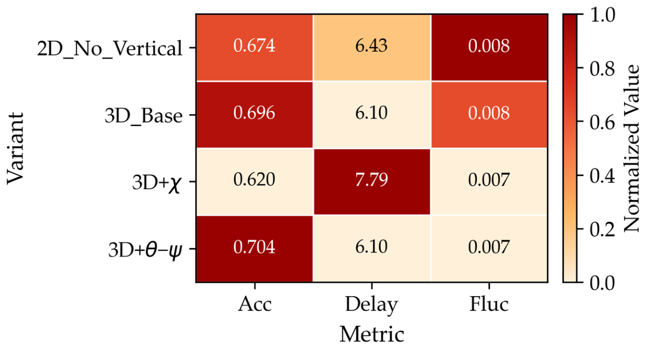
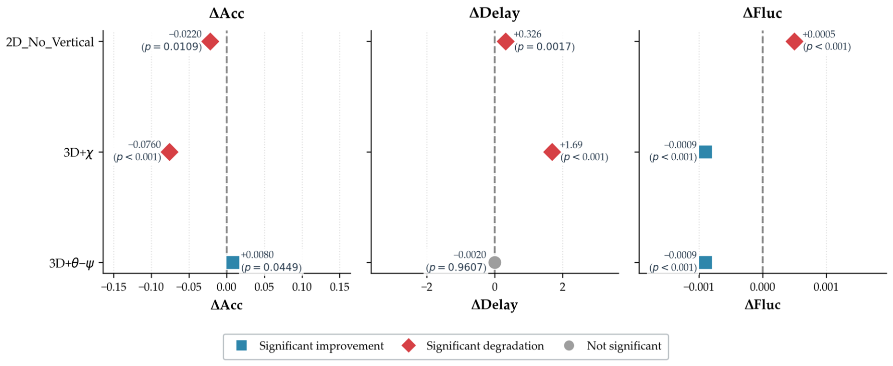
As shown in

Table 14. Results of the 3D-factor ablation study.

Variant	Acc	Delay (s)	Fluc
2D_No_Vertical	0.674	6.43	0.0082
3D_Base	0.696	6.10	0.0077
3D + χ	0.620	7.79	0.0068
3D + θ − ψ	0.704	6.10	0.0068

and

Table 15. Paired statistical results relative to 3D_Base.

Variant	ΔAcc	p (Acc)	ΔDelay (s)	p (Delay)	ΔFluc	p (Fluc)
2D_No_Vertical	−0.0220	0.0109	+0.3260	0.0017	+0.0005	<0.0001
3D + χ	−0.0760	<0.0001	+1.6880	<0.0001	−0.0009	<0.0001
3D + θ − ψ	+0.0080	0.0449	−0.0020	0.9607	−0.0009	<0.0001

and Figure 12 and Figure 13, 3D_Base clearly outperforms 2D_No_ Vertical. After altitude difference and vertical-approach information are introduced, accuracy increases and response delay decreases, with statistically significant differences. This confirms that 3D factors make a substantive contribution to low-altitude UAV threat assessment rather than merely adding redundant features.

The 3D + θ − ψ variant further improves accuracy and reduces Fluc relative to 3D_Base. This indicates that attitude information can effectively complement velocity directionality. In particular, during low-speed motion, turning maneuvers, or short-term disturbances, body orientation may be more stable than instantaneous velocity direction and can therefore improve threat ranking. Although the response delay is nearly unchanged, the improvements in accuracy and stability suggest that attitude information has practical value when reliable attitude observations are available.

Compared with 3D_Base, the 3D + χ variant exhibits a decrease in accuracy (Δ = −0.076, p < 0.0001), an increase in response delay (Δ = +1.688, p < 0.0001), and a moderate reduction in Fluc (Δ = −0.0009, p < 0.0001). These results indicate that the reachability coefficient alters the output characteristics of the threat assessment model. By incorporating obstacle-constraint information, the coefficient assigns more conservative threat scores to UAVs whose direct approach paths are obstructed, thereby producing a smoother threat sequence at the expense of a somewhat slower response to certain dynamic approaching behaviors.

From a functional perspective, the reachability coefficient provides the proposed framework with a mechanism for integrating environmental constraints into threat assessment. When obstacles block the direct line of sight between a UAV and a protected asset, this coefficient reflects the degree of path obstruction and adjusts the threat score accordingly, allowing the assessment to depend not only on geometric proximity but also on spatial accessibility. This capability is of potential practical value in obstacle-rich scenarios such as low-altitude urban environments, mountainous terrain, and indoor spaces.

4.11. Discussion of Experimental Results

The experimental results demonstrate that the proposed method achieves a better balance between response sensitivity and temporal stability than the comparison methods. By evaluating threats at the UAV–protected asset pair level, the proposed threat matrix preserves the many-to-many relationship between UAVs and protected assets, which is essential for multi-asset low-altitude safety monitoring. This matrix-form representation enables each protected asset to identify its dominant UAV threats while supporting an overall interpretation of the monitoring situation. The performance improvement is mainly attributed to the combined use of approach directionality, history-based trend correction, and adaptive EMA smoothing. The directionality factor enhances sensitivity to UAVs moving toward a protected asset, the trend correction factor incorporates temporal evidence of persistent threat evolution, and the adaptive smoothing mechanism reduces noise-induced score fluctuations without excessively delaying meaningful changes. Together, these components improve threat-score consistency and reduce unnecessary ranking switches. The ablation and baseline comparisons further confirm the role of each component. Methods without directionality show weaker threat discrimination, whereas trend correction without temporal smoothing remains vulnerable to local perturbations. Fixed smoothing, on the other hand, cannot adapt to different dynamic conditions. Although TOPSIS offers a conventional multi-attribute decision-making baseline, it does not explicitly model temporal evolution, and its scores are relative to the current decision matrix. Therefore, it is less suitable for capturing continuous threat development over time. The ablation results confirm that the key novelty is not the trend correction or the EMA smoothing alone, but their coupling: trend correction without smoothing amplifies noise, smoothing without trend awareness delays response, and only their adaptive combination achieves the demonstrated balance.

The systematic comparison between the 2D and 3D variants (Section 4.2 and Section 4.10) confirms that three-dimensional factors—altitude difference, vertical approach velocity, and attitude angle coupling—are not redundant additions but essential for reliable threat discrimination in realistic low-altitude airspace. The 2D model’s systematic failure in vertical-approach scenarios highlights the necessity of explicit 3D kinematics in UAV threat assessment for safety monitoring.

The present study is based on simulation experiments, which allow systematic evaluation across a wide range of parameterized scenarios. While the degradation experiments in Section 4.7 examine several non-ideal factors—latency, missed detections, clutter, and suboptimal filtering—these are synthetically injected at controlled levels; further validation using recorded sensor data and field tests would provide complementary evidence under more complex practical conditions. The proposed method is best suited for scenarios with relatively stable directional trends; in highly dynamic or adversarial multi-UAV environments, the linear trend model and the independent pairwise evaluation may reach their limits, as the difficult-case analysis in Section 4.8 suggests.

These results demonstrate the potential of the proposed method for real-time multi-asset UAV safety monitoring, particularly in applications requiring explainability, stable ranking, and prompt response.

5. Conclusions

This study developed an interpretable three-dimensional dynamic threat assessment framework for multi-asset UAV safety monitoring. By treating each UAV–asset pair as an assessment unit, the framework represents many-to-many threat relationships in matrix form and supports both asset-specific UAV ranking and identification of the asset most likely threatened by each UAV. The proposed method combines three-dimensional threat factors, approach directionality, historical-trend correction, and adaptive exponential smoothing to balance dynamic responsiveness and temporal stability.

The simulation results show that three-dimensional information, particularly altitude difference and vertical approach velocity, is important for distinguishing UAVs that exhibit similar horizontal motion but different vertical approach behaviors. Directionality improves the identification of UAVs moving toward protected assets, whereas adaptive smoothing substantially reduces noise-induced score fluctuations and unnecessary ranking changes. The results also show that trend correction alone does not necessarily improve stability; its benefit emerges when it is coupled with adaptive temporal smoothing. Compared with fixed smoothing, the proposed method provides a different trade-off, with slightly improved responsiveness and identification performance in the tested scenarios, although fixed smoothing yields marginally lower fluctuation in some cases.

Future work will pursue two main directions: (i) validation using real UAV flight data and sensor measurements to complement the current simulation-based evaluation; and (ii) integration of the threat matrix with downstream resource allocation and active monitoring strategies for operational deployment.

References

1. Hassanalian, M.; Abdelkefi, A. Classifications, applications, and design challenges of drones: A review. Prog. Aerosp. Sci. 2017, 91, 99–131. [Google Scholar] [CrossRef]
2. Mohsan, S.A.H.; Othman, N.Q.H.; Li, Y.; Alsharif, M.H.; Khan, M.A. Unmanned aerial vehicles (UAVs): Practical aspects, applications, open challenges, security issues, and future trends. Intell. Serv. Robot. 2023, 16, 109–137. [Google Scholar] [CrossRef] [PubMed]
3. Shakhatreh, H.; Sawalmeh, A.H.; Al-Fuqaha, A.; Dou, Z.; Almaita, E.; Khalil, I.; Othman, N.S.; Khreishah, A.; Guizani, M. Unmanned Aerial Vehicles (UAVs): A Survey on Civil Applications and Key Research Challenges. IEEE Access 2019, 7, 48572–48634. [Google Scholar] [CrossRef]
4. Guvenc, I.; Koohifar, F.; Singh, S.; Sichitiu, M.L.; Matolak, D. Detection, Tracking, and Interdiction for Amateur Drones. IEEE Commun. Mag. 2018, 56, 75–81. [Google Scholar] [CrossRef]
5. Lykou, G.; Moustakas, D.; Gritzalis, D. Defending Airports from UAS: A Survey on Cyber-Attacks and Counter-Drone Sensing Technologies. Sensors 2020, 20, 3537. [Google Scholar] [CrossRef] [PubMed]
6. Park, S.; Kim, H.T.; Lee, S.; Joo, H.; Kim, H. Survey on Anti-Drone Systems: Components, Designs, and Challenges. IEEE Access 2021, 9, 42635–42659. [Google Scholar] [CrossRef]
7. Taha, B.; Shoufan, A. Machine Learning-Based Drone Detection and Classification: State-of-the-Art in Research. IEEE Access 2019, 7, 138669–138682. [Google Scholar] [CrossRef]
8. Yaacoub, J.P.; Noura, H.; Salman, O.; Chehab, A. Security analysis of drones systems: Attacks, limitations, and recommendations. Internet Things 2020, 11, 100218. [Google Scholar] [CrossRef] [PubMed]
9. Coluccia, A.; Fascista, A.; Schumann, A.; Sommer, L.; Dimou, A.; Zarpalas, D.; Mendez, M.; de la Iglesia, D.; Gonzalez, I.; Mercier, J.P.; et al. Drone vs. Bird Detection: Deep Learning Algorithms and Results from a Grand Challenge. Sensors 2021, 21, 2824. [Google Scholar] [CrossRef] [PubMed]
10. Shi, X.; Yang, C.; Xie, W.; Liang, C.; Shi, Z.; Chen, J. Anti-Drone System with Multiple Surveillance Technologies: Architecture, Implementation, and Challenges. IEEE Commun. Mag. 2018, 56, 68–74. [Google Scholar] [CrossRef]
11. Benavoli, A.; Ristic, B.; Farina, A.; Oxenham, M.; Chisci, L. An approach to threat assessment based on evidential networks. In Proceedings of the 2007 10th International Conference on Information Fusion, Quebec, QC, Canada, 9–12 July 2007, 2007; pp. 1–8. [Google Scholar]
12. Wang, Y.; Liu, S.; Niu, W.; Liu, K.; Liao, Y. Threat assessment method based on intuitionistic fuzzy similarity measurement reasoning with orientation. China Commun. 2014, 11, 119–128. [Google Scholar] [CrossRef]
13. Fan, C.; Fu, Q.; Song, Y.; Lu, Y.; Li, W.; Zhu, X. A New Model of Interval-Valued Intuitionistic Fuzzy Weighted Operators and Their Application in Dynamic Fusion Target Threat Assessment. Entropy 2022, 24, 1825. [Google Scholar] [CrossRef] [PubMed]
14. Di, R.; Gao, X.; Guo, Z.; Wan, K. A Threat Assessment Method for Unmanned Aerial Vehicle Based on Bayesian Networks under the Condition of Small Data Sets. Math. Probl. Eng. 2018, 2018, 8484358. [Google Scholar] [CrossRef]
15. Zhang, K.; Kong, W.; Liu, P.; Shi, J.; Lei, Y.; Zou, J. Assessment and sequencing of air target threat based on intuitionistic fuzzy entropy and dynamic VIKOR. J. Syst. Eng. Electron. 2018, 29, 305–310. [Google Scholar] [CrossRef]
16. Pires, H.B.; Guimarães, L.N.F. Dynamic Multi-Target Three-Way Threat Assessment in the Context of Air Defense. IEEE Access 2024, 12, 141397–141413. [Google Scholar] [CrossRef]
17. Niu, Q.; Ren, S.; Gao, W.; Wang, C. A Dynamic Threat Assessment Method for Multi-Target Unmanned Aerial Vehicles at Multiple Time Points Based on Fuzzy Multi-Attribute Decision Making and Fuse Intention. Mathematics 2025, 13, 1663. [Google Scholar] [CrossRef]
18. Ma, S.; Zhang, H.; Yang, G. Target threat level assessment based on cloud model under fuzzy and uncertain conditions in air combat simulation. Aerosp. Sci. Technol. 2017, 67, 49–53. [Google Scholar] [CrossRef]
19. Yu, X.; Wei, S.; Fang, Y.; Sheng, J.; Zhang, L. Low-Altitude Slow Small Target Threat Assessment Algorithm by Exploiting Sequential Multifeature With Long Short-Term Memory. IEEE Sens. J. 2023, 23, 21524–21533. [Google Scholar] [CrossRef]
20. Jiang, D.; Dong, Y.; Zhang, L.; Lu, X.; Dong, C. Research on Air Target Threat Assessment Technology Based on Deep Learning. J. Syst. Simul. 2025, 37, 791–802. [Google Scholar] [CrossRef]
21. Zhang, H.; Yan, Y.; Li, S.; Hu, Y.; Liu, H. UAV Behavior-Intention Estimation Method Based on 4-D Flight-Trajectory Prediction. Sustainability 2021, 13, 12528. [Google Scholar] [CrossRef]
22. Wang, Z.; Chen, J.; Wang, J.; Shen, Q. Intention recognition of UAV swarm with data-driven methods. Aerosp. Syst. 2023, 6, 703–714. [Google Scholar] [CrossRef]
23. Shukla, P.; Shukla, S.; Kumar Singh, A. Trajectory-Prediction Techniques for Unmanned Aerial Vehicles (UAVs): A Comprehensive Survey. IEEE Commun. Surv. Tutor. 2025, 27, 1867–1910. [Google Scholar] [CrossRef]
24. Castrillo, V.U.; Manco, A.; Pascarella, D.; Gigante, G. A Review of Counter-UAS Technologies for Cooperative Defensive Teams of Drones. Drones 2022, 6, 65. [Google Scholar] [CrossRef]
25. Arapoglou, F.; Zacharia, P.; Papoutsidakis, M. Intelligent Counter-UAV Threat Detection Using Hierarchical Fuzzy Decision-Making and Sensor Fusion. Sensors 2025, 25, 6091. [Google Scholar] [CrossRef] [PubMed]
26. Semenyuk, V.; Kurmashev, I.; Lupidi, A.; Alyoshin, D.; Kurmasheva, L.; Cantelli-Forti, A. Advances in UAV detection: Integrating multi-sensor systems and AI for enhanced accuracy and efficiency. Int. J. Crit. Infrastruct. Prot. 2025, 49, 100744. [Google Scholar] [CrossRef]
27. Qin, Z.; Wang, L.; Zhou, S.; Fu, P.; Hua, G.; Tang, W. Towards Generalizable Multi-Object Tracking. In Proceedings of the 2024 IEEE/CVF Conference on Computer Vision and Pattern Recognition (CVPR), Washington, DC, USA, 17–24 June 2024; pp. 18995–19004. [Google Scholar]
28. Farrera, B.; López-Estrada, F.-R.; Chadli, M.; Valencia-Palomo, G.; Gómez-Peñate, S. Distributed fault estimation of multi-agent systems using a proportional-integral observer: A leader-following application. Int. J. Appl. Math. Comput. Sci. 2020, 30, 551–560. [Google Scholar] [CrossRef]
29. Vazquez Trejo, J.A.; Ponsart, J.-C.; Adam-Medina, M.; Valencia-Palomo, G. Fault-tolerant observer-based leader-following consensus control for LPV multi-agent systems using virtual actuators. Int. J. Syst. Sci. 2024, 56, 1816–1833. [Google Scholar] [CrossRef]
30. Saaty, T.L. The Analytic Hierarchy Process: Decision Making in Complex Environments. In Quantitative Assessment in Arms Control; Springer: Boston, MA, USA, 1984; pp. 285–308. [Google Scholar]
31. Hwang, C.-L.; Yoon, K. Multiple Attribute Decision Making Methods and Applications; Springer-Verlag: Berlin/Heidelberg, Germany, 1981. [Google Scholar]
32. Opricovic, S.; Tzeng, G.-H. Compromise solution by MCDM methods: A comparative analysis of VIKOR and TOPSIS. Eur. J. Oper. Res. 2004, 156, 445–455. [Google Scholar] [CrossRef]
33. Yin, Y.; Zhang, R.; Su, Q. Threat assessment of aerial targets based on improved GRA-TOPSIS method and three-way decisions. Math. Biosci. Eng. 2023, 20, 13250–13266. [Google Scholar] [CrossRef] [PubMed]
34. Zhang, J.; Shan, Y.; Dong, J. A threat assessment method based on correlation-similarity information and three-way decisions in interval intuitionistic fuzzy environment. Eng. Appl. Artif. Intell. 2024, 135, 108793. [Google Scholar] [CrossRef]
35. Gao, Y.; Lyu, N. A New Multi-Target Three-Way Threat Assessment Method with Heterogeneous Information and Attribute Relevance. Mathematics 2024, 12, 691. [Google Scholar] [CrossRef]
36. Girase, H.; Gang, H.; Malla, S.; Li, J.; Kanehara, A.; Mangalam, K.; Choi, C. LOKI: Long Term and Key Intentions for Trajectory Prediction. In Proceedings of the 2021 IEEE/CVF International Conference on Computer Vision (ICCV), Virtual, 11–17 October 2021; pp. 9783–9792. [Google Scholar]
37. Chen, W.; He, F.; Dong, H. Maneuvering target tracking based on an adaptive variable structure interactive multiple model filtering and smoothing algorithm. AIP Adv. 2023, 13, 045307. [Google Scholar] [CrossRef]
38. Hu, K.Y.; Wang, J.; Cheng, Y.; Yang, C. Adaptive filtering and smoothing algorithm based on variable structure interactive multiple model. Sci. Rep. 2023, 13, 12993. [Google Scholar] [CrossRef] [PubMed]
39. Wang, Y.; Li, R.; Zhang, D.; Li, M.; Cao, J.; Zheng, Z. CATrack: Condition-aware multi-object tracking with temporally enhanced appearance features. Knowl.-Based Syst. 2025, 308, 112760. [Google Scholar] [CrossRef]
40. Demsar, J. Statistical comparisons of classifiers over multiple data sets. J. Mach. Learn. Res. 2006, 7, 1–30. [Google Scholar]
Figure 1. Schematic illustration of UAV threat scenarios.
Drones 10 00536 g001
Figure 2. Evaluation flowchart of the proposed model.
Drones 10 00536 g002
Figure 3. Illustration of instantaneous approach directionality.
Drones 10 00536 g003
Figure 4. History-based directionality correction: 3D trajectory colored by instantaneous directionality, with velocity (blue) and asset-direction (red) vectors.
Drones 10 00536 g004
Figure 5. Performance comparison of the dynamic Monte Carlo experiment.
Drones 10 00536 g005
Figure 6. Paired differences between Proposed and Inst with 95% confidence intervals and Cohen’s d.
Drones 10 00536 g006
Figure 7. Performance of Inst, Raw, and Proposed under different noise levels.
Drones 10 00536 g007
Figure 8. Heatmaps of paired differences in the noise robustness experiment.
Drones 10 00536 g008
Figure 9. Parameter sensitivity analysis of the proposed method.
Drones 10 00536 g009
Figure 10. Paired performance comparison between Proposed and Inst under practical observation degradation.
Drones 10 00536 g010
Figure 11. Diverging point chart of absolute sensitivity of the proposed method to degradation conditions.
Drones 10 00536 g011
Figure 12. Heatmap of the 3D-factor ablation study.
Drones 10 00536 g012
Figure 13. Paired comparison of ablation variants relative to 3D_Base with p-values.
Drones 10 00536 g013