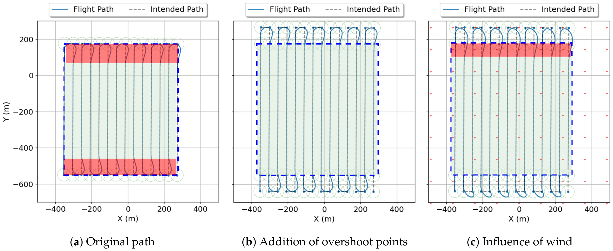
Figure 1.
Comparison of how overshoot points can improve effective coverage and how wind effects amplify deviations (area of interest (AOI): dashed blue line; effective coverage: green zone; compromised region: red zone).
Figure 1.
Comparison of how overshoot points can improve effective coverage and how wind effects amplify deviations (area of interest (AOI): dashed blue line; effective coverage: green zone; compromised region: red zone).
Figure 2.
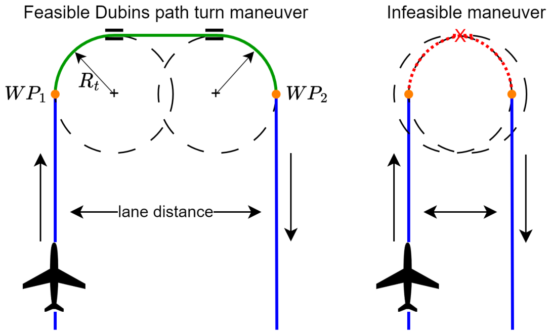
Dubins path (Bang–Singular–Bang [BSB]) in a turn maneuver between two alternating lanes becomes infeasible as the lane distance decreases.
Figure 2.
Dubins path (Bang–Singular–Bang [BSB]) in a turn maneuver between two alternating lanes becomes infeasible as the lane distance decreases.
Figure 3.
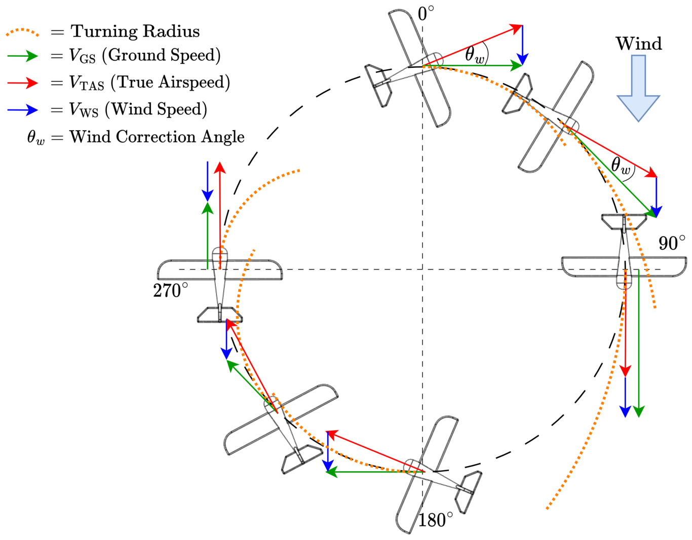
Variation in ground speed during constant true airspeed , with constant-bank turns under wind influence.
Figure 3.
Variation in ground speed during constant true airspeed , with constant-bank turns under wind influence.
Figure 4.
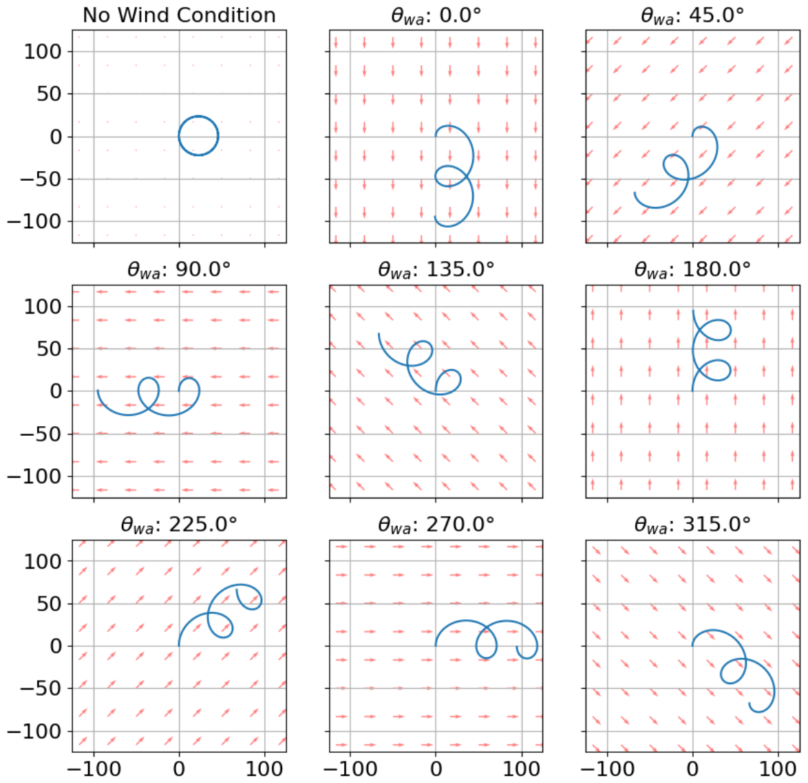
Trochoidal paths for a full right-hand turn at m/s and under different wind bearings.
Figure 4.
Trochoidal paths for a full right-hand turn at m/s and under different wind bearings.
Figure 5.
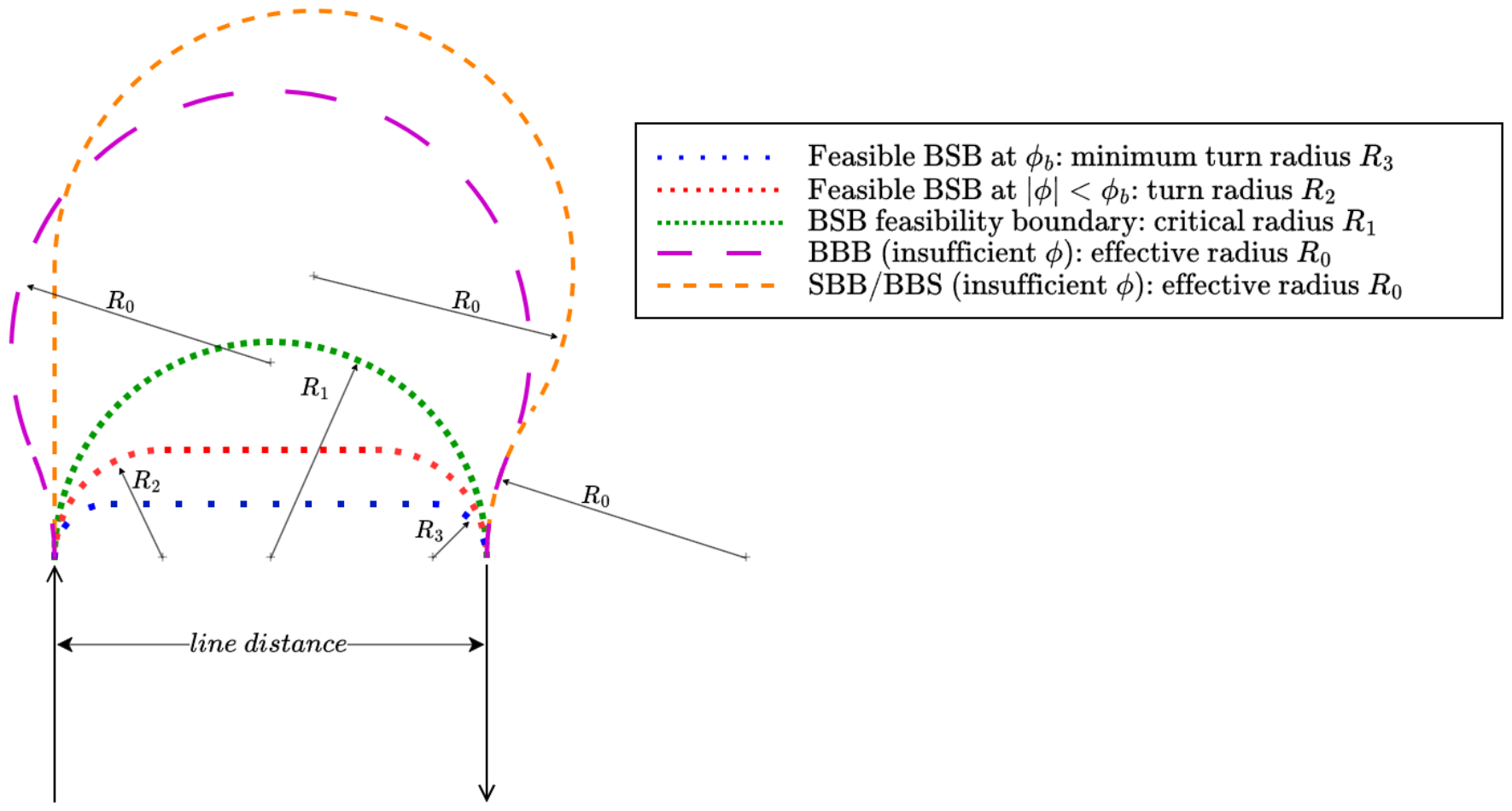
Possible turning strategies for a right-turn lane-change maneuver. Dotted curves illustrate standard feasible BSB maneuver; dashed curves indicate Singular–Bang–Bang (SBB)/Bang–Bang–Singular (BBS) and Bang–Bang–Bang (BBB) extensions used when the available bank angle is insufficient for a feasible BSB maneuver.
Figure 5.
Possible turning strategies for a right-turn lane-change maneuver. Dotted curves illustrate standard feasible BSB maneuver; dashed curves indicate Singular–Bang–Bang (SBB)/Bang–Bang–Singular (BBS) and Bang–Bang–Bang (BBB) extensions used when the available bank angle is insufficient for a feasible BSB maneuver.
Figure 6.
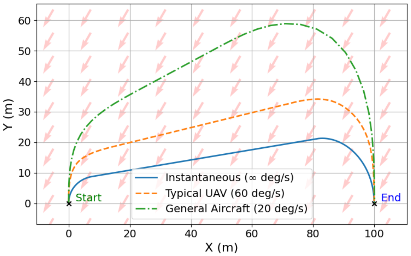
Optimal lane-change ground tracks for different roll-rate limits (, , and ) for the maneuver from to at m/s and m/s from (red arrows indicate wind direction).
Figure 6.
Optimal lane-change ground tracks for different roll-rate limits (, , and ) for the maneuver from to at m/s and m/s from (red arrows indicate wind direction).
Figure 7.
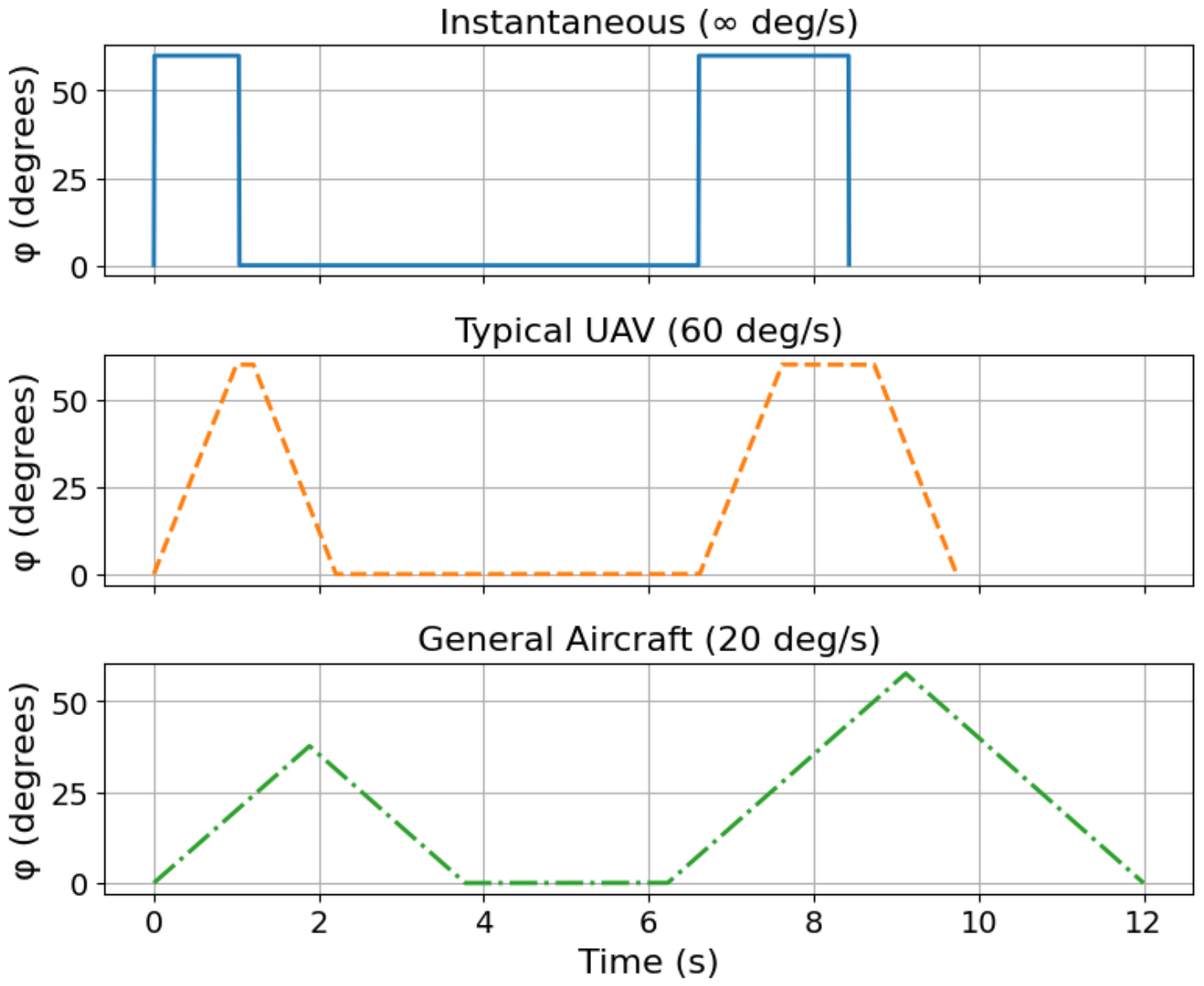
Distribution of bank-angle usage for different roll-rate limits, showing the fraction of maneuver time spent at intermediate banks versus the commanded maximum .
Figure 7.
Distribution of bank-angle usage for different roll-rate limits, showing the fraction of maneuver time spent at intermediate banks versus the commanded maximum .
Figure 8.
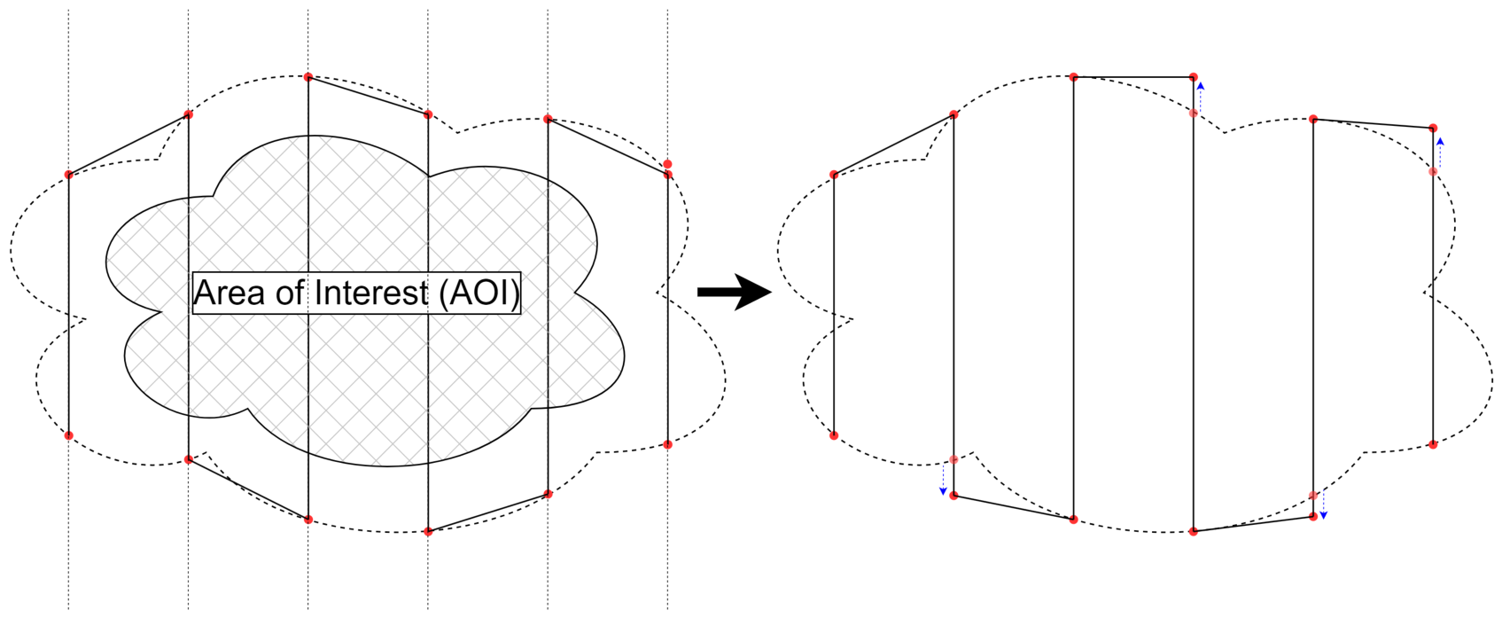
Boustrophedon path formulation to ensure equal footprints within the AOI. The dashed boundary denotes the buffer region added to the AOI, whereas the red points represent waypoints that can be extended outward (indicated by blue arrows on the right-hand side figure) to ensure complete coverage by the boustrophedon path.
Figure 8.
Boustrophedon path formulation to ensure equal footprints within the AOI. The dashed boundary denotes the buffer region added to the AOI, whereas the red points represent waypoints that can be extended outward (indicated by blue arrows on the right-hand side figure) to ensure complete coverage by the boustrophedon path.
Figure 9.
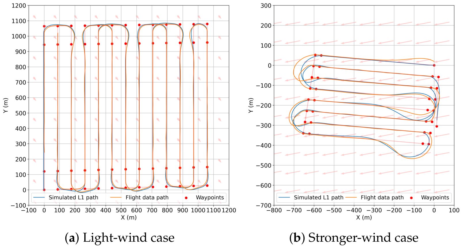
Trajectory-level comparison between the simulated path and the logged Raybe flight path under different wind conditions.
Figure 9.
Trajectory-level comparison between the simulated path and the logged Raybe flight path under different wind conditions.
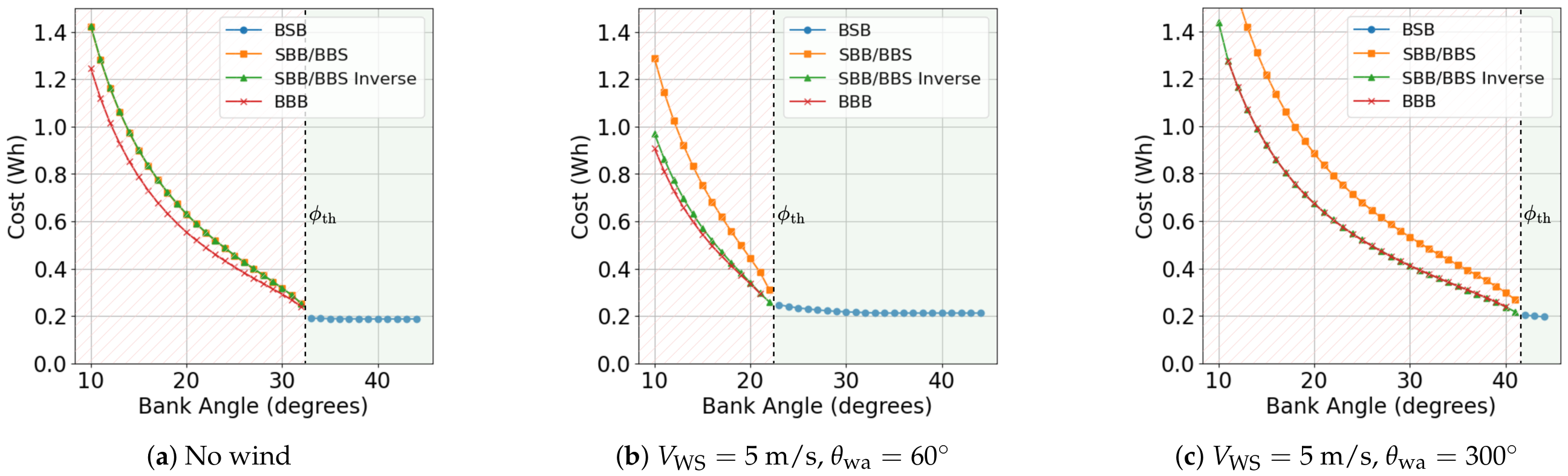
Figure 10.
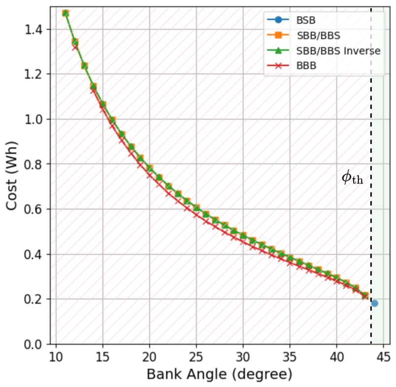
Energy cost (Wh) versus bank angle (deg) for a full right-turn maneuver under three wind conditions: no wind, wind from , and wind from .
Figure 10.
Energy cost (Wh) versus bank angle (deg) for a full right-turn maneuver under three wind conditions: no wind, wind from , and wind from .
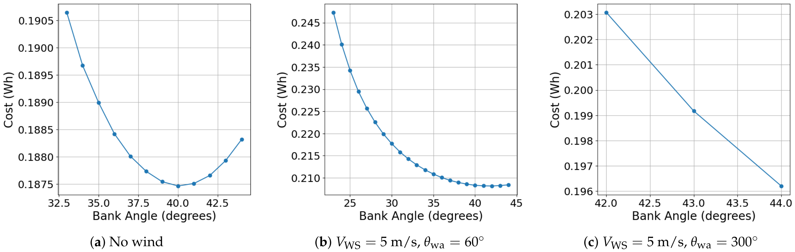
Figure 11.
Energy cost for BSB maneuvers under three wind conditions within the
sufficient bank-angle zone; only the green-shaded zone of
Figure 10 is shown here.
Figure 11.
Energy cost for BSB maneuvers under three wind conditions within the
sufficient bank-angle zone; only the green-shaded zone of
Figure 10 is shown here.
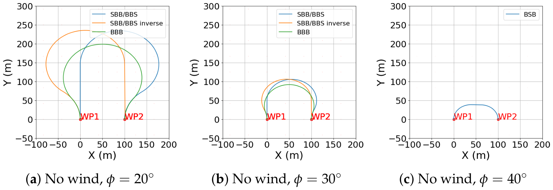
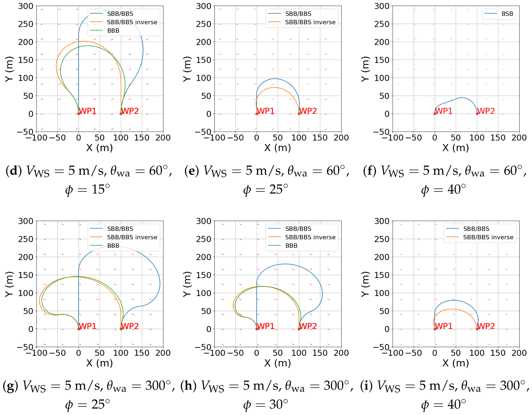
Figure 12.
Maneuver paths for a full right turn under different wind conditions and bank angles.
Figure 12.
Maneuver paths for a full right turn under different wind conditions and bank angles.
Figure 13.
Impact of crosswind (5 m/s from ) on energy cost at different bank angles for a full right-turn maneuver.
Figure 13.
Impact of crosswind (5 m/s from ) on energy cost at different bank angles for a full right-turn maneuver.
Figure 14.
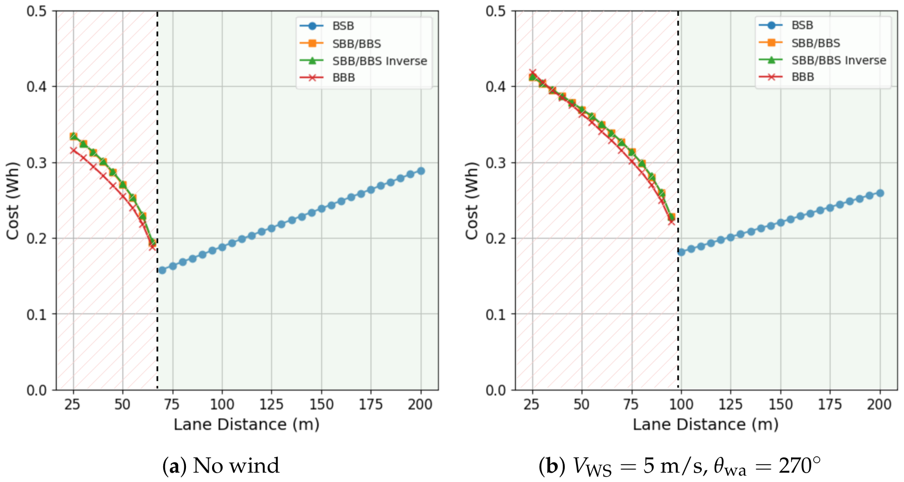
Energy cost as a function of lane distance for a full right-turn maneuver under no wind and crosswind conditions. Green shading indicates the sufficient bank-angle (BSB-feasible) zone, and red hatching indicates the insufficient bank-angle zone.
Figure 14.
Energy cost as a function of lane distance for a full right-turn maneuver under no wind and crosswind conditions. Green shading indicates the sufficient bank-angle (BSB-feasible) zone, and red hatching indicates the insufficient bank-angle zone.
Figure 15.
Boustrophedon path evaluation across various flight path angles for the axisymmetric AOI.
Figure 15.
Boustrophedon path evaluation across various flight path angles for the axisymmetric AOI.
Figure 16.
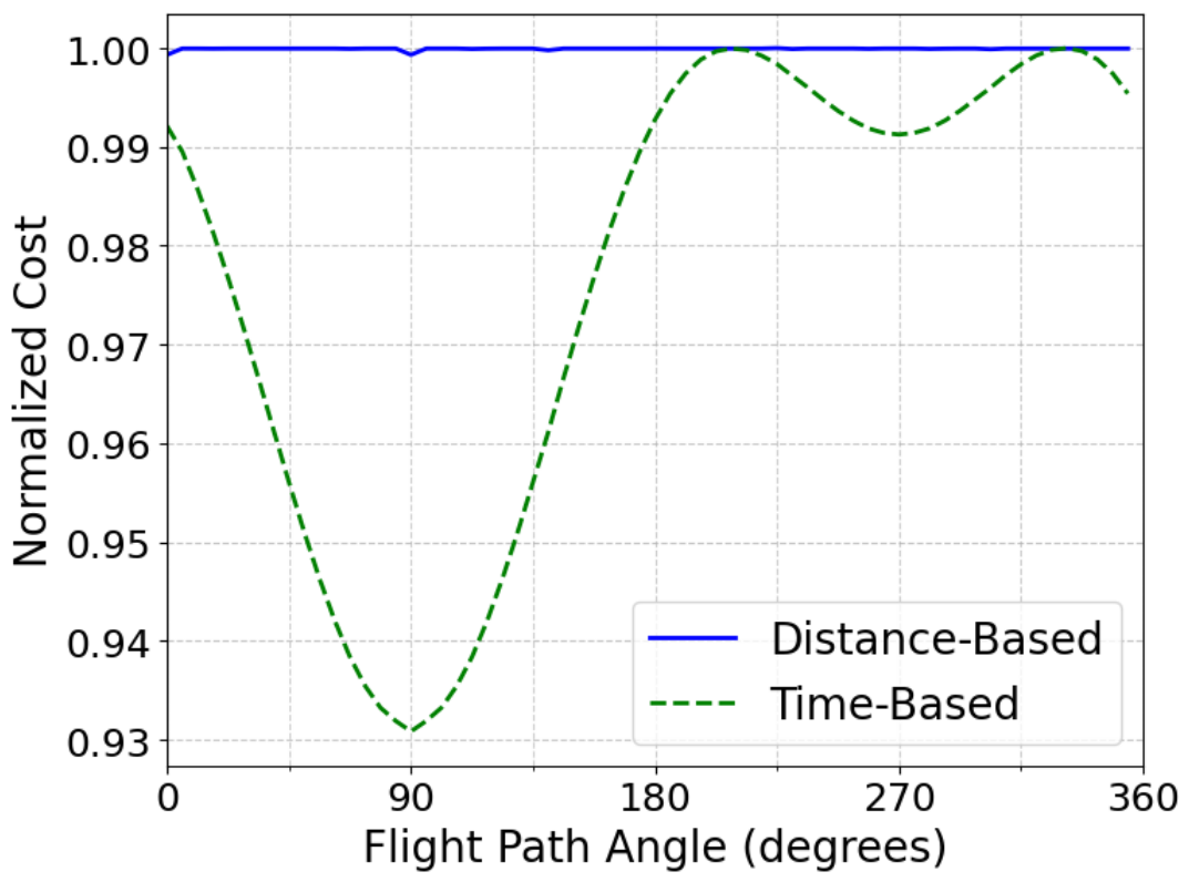
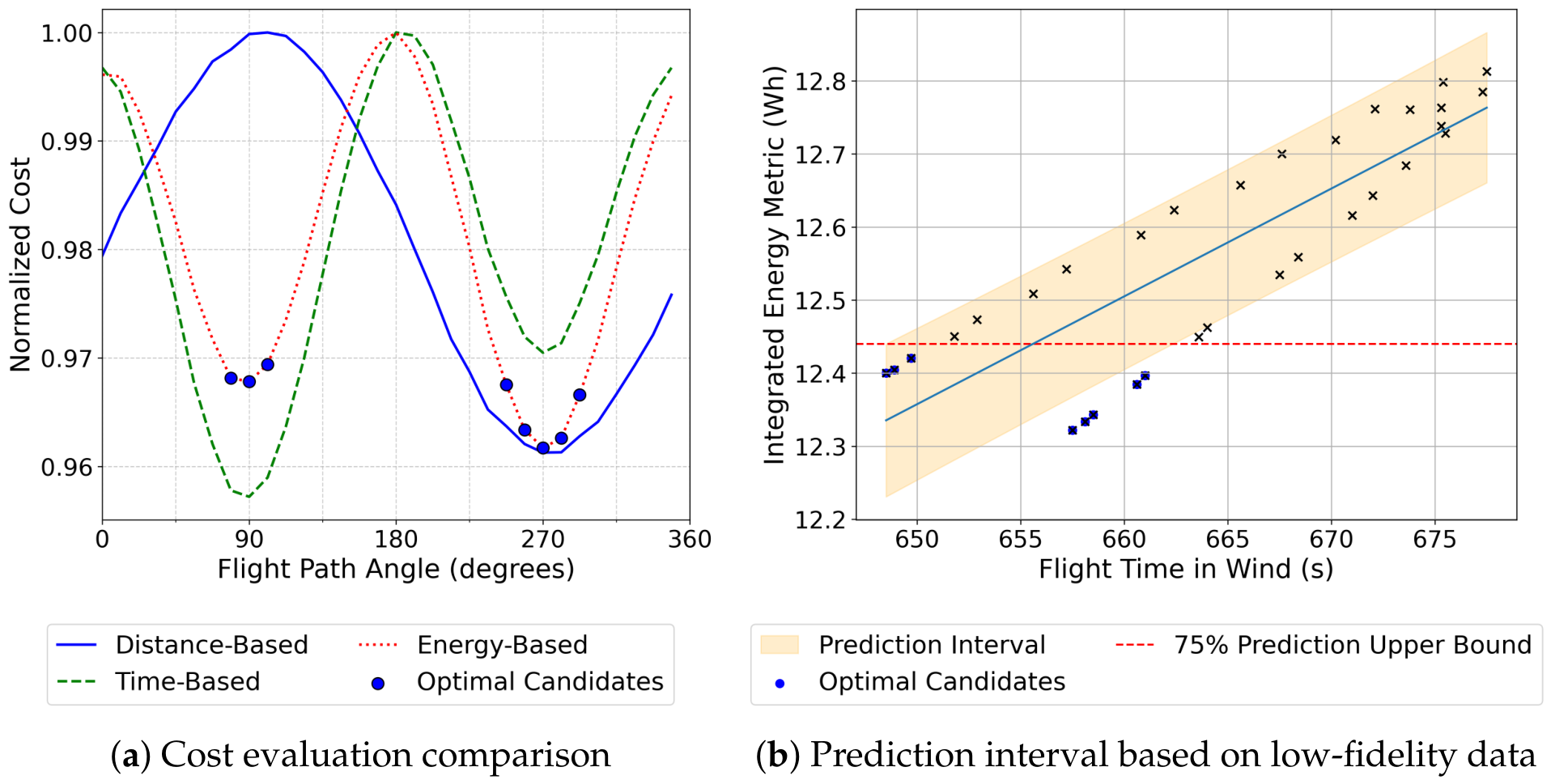
Comparison of distance-based and time-based cost evaluations for boustrophedon paths in the axisymmetric AOI.
Figure 16.
Comparison of distance-based and time-based cost evaluations for boustrophedon paths in the axisymmetric AOI.
Figure 17.
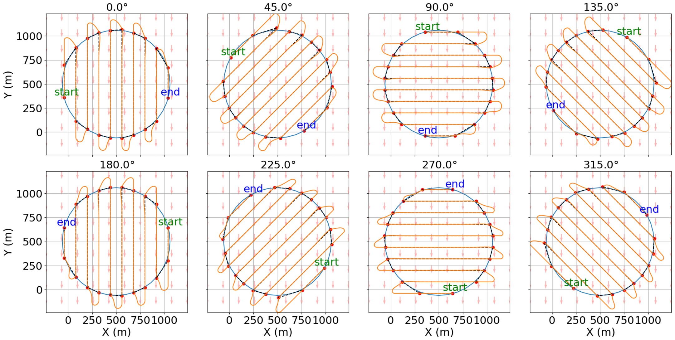
Simulated flight path results using control, with additional overshoot points at the end of each lane in the axisymmetric AOI.
Figure 17.
Simulated flight path results using control, with additional overshoot points at the end of each lane in the axisymmetric AOI.
Figure 18.
Performance evaluation of aerial mapping tasks over an axisymmetric AOI.
Figure 18.
Performance evaluation of aerial mapping tasks over an axisymmetric AOI.
Figure 19.
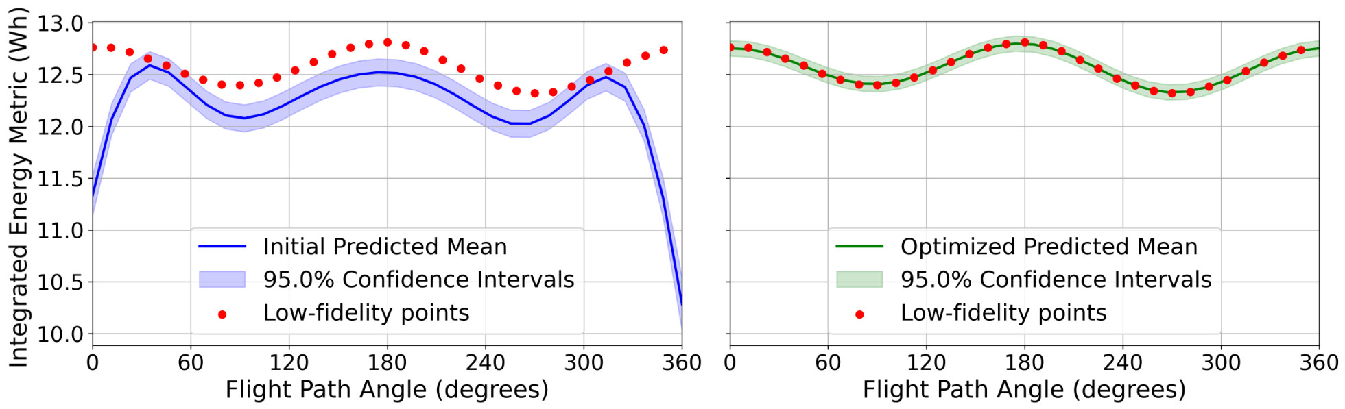
Gaussian process (GP) surrogate for low-fidelity Integrated Energy Metric (IEM) versus path angle (axisymmetric AOI): initial fit (left) and refined fit (right), showing posterior mean and 95% confidence intervals.
Figure 19.
Gaussian process (GP) surrogate for low-fidelity Integrated Energy Metric (IEM) versus path angle (axisymmetric AOI): initial fit (left) and refined fit (right), showing posterior mean and 95% confidence intervals.
Figure 20.
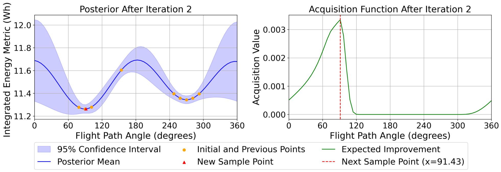
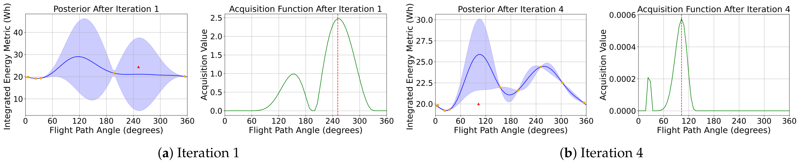
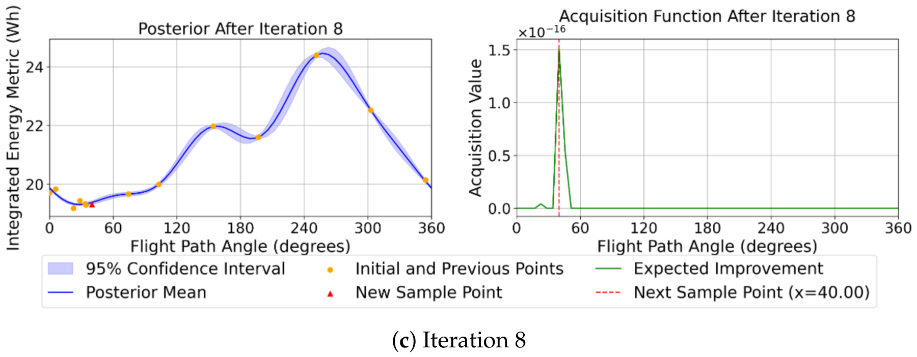
Posterior distribution and acquisition function after the second Bayesian optimization (BO) iteration (axisymmetric AOI).
Figure 20.
Posterior distribution and acquisition function after the second Bayesian optimization (BO) iteration (axisymmetric AOI).
Figure 21.
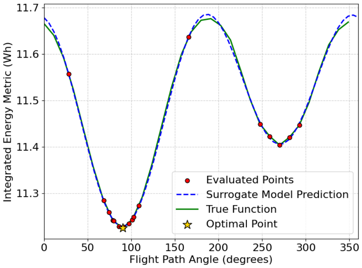
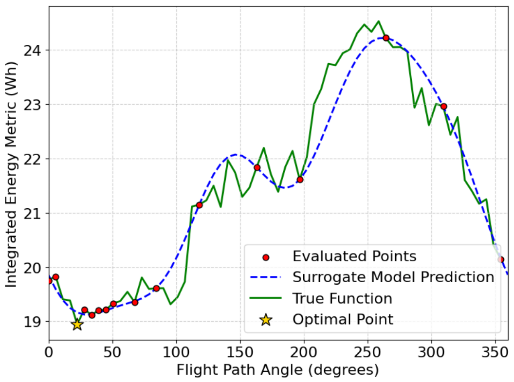
Comparison between exhaustive evaluation (true function) and BO optimization results for Test Case 2.
Figure 21.
Comparison between exhaustive evaluation (true function) and BO optimization results for Test Case 2.
Figure 22.
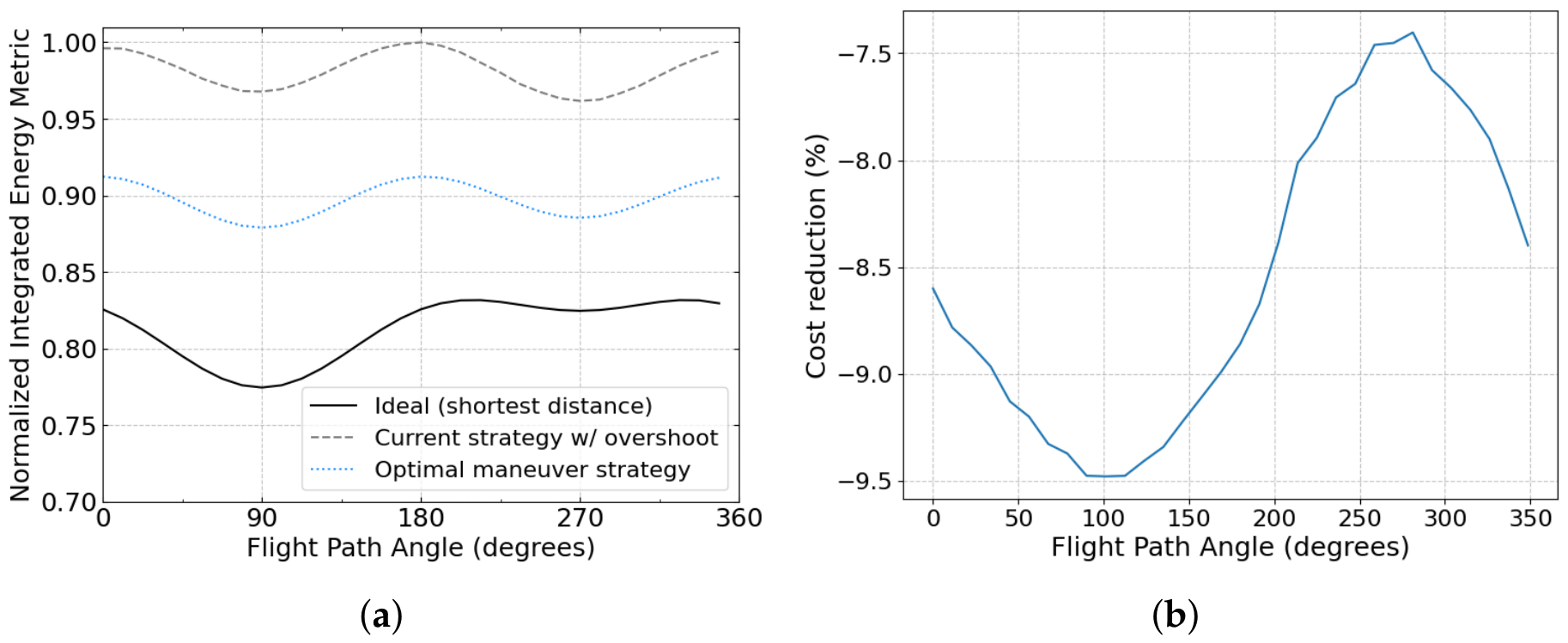
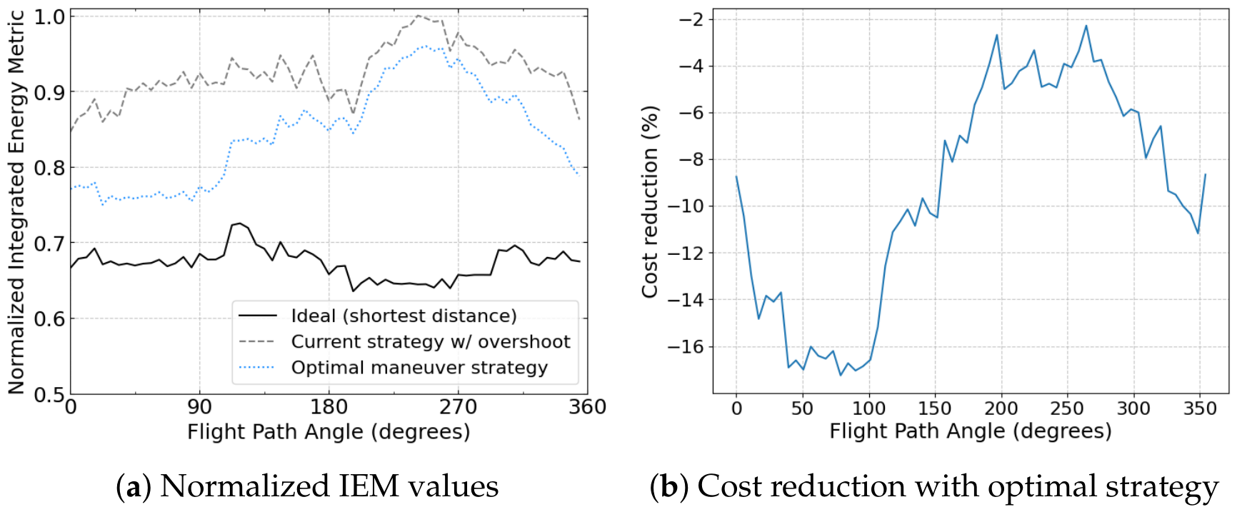
IEM comparison for Test Case 2 under different strategies. (a) Comparison of normalized IEM values. (b) IEM reduction achieved by the optimal strategy.
Figure 22.
IEM comparison for Test Case 2 under different strategies. (a) Comparison of normalized IEM values. (b) IEM reduction achieved by the optimal strategy.
Figure 23.
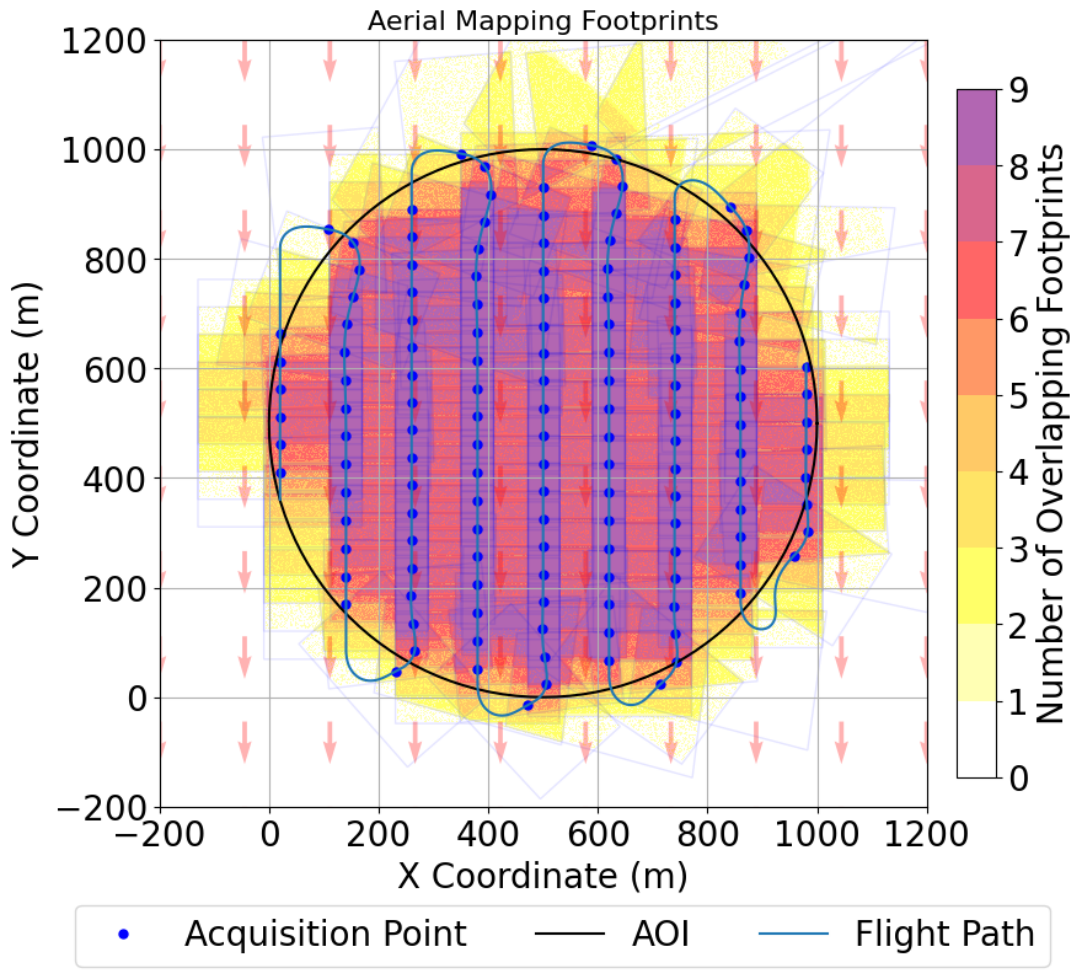
Baseline footprint-overlap map for the conventional maneuver without overshoot points and without buffer at path angle for Test Case 2.
Figure 23.
Baseline footprint-overlap map for the conventional maneuver without overshoot points and without buffer at path angle for Test Case 2.
Figure 24.
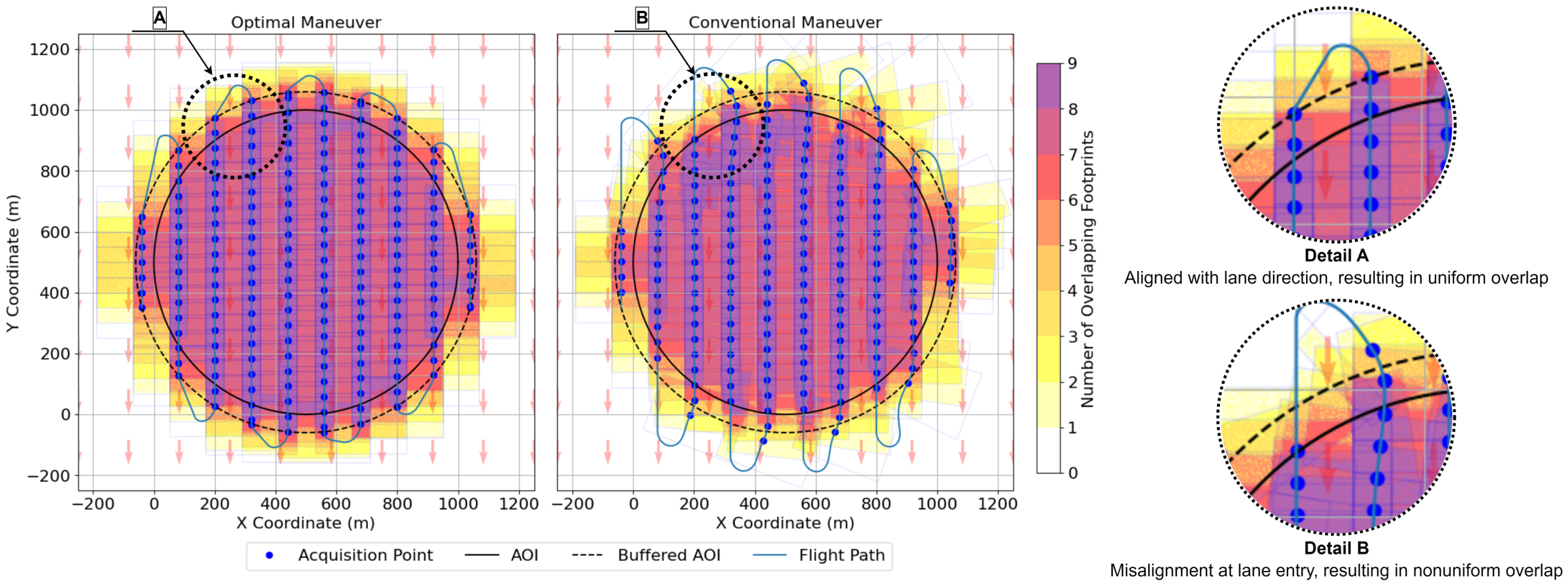
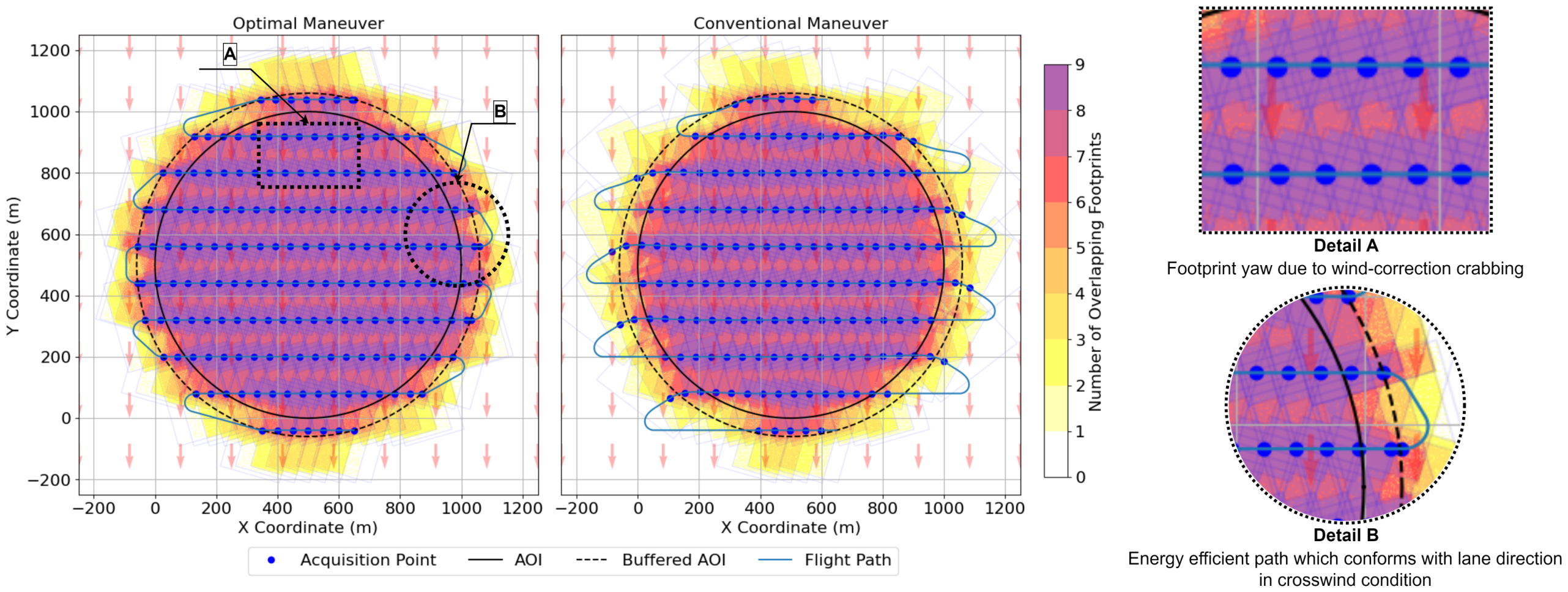
Comparison of image footprints for the optimal and conventional maneuver strategies at a path angle for Test Case 2. Details A and B magnify representative lane-entry regions: A shows the optimized maneuver aligned with the lane direction and producing uniform overlap, whereas B shows conventional lane-entry misalignment and local non-uniform overlap.
Figure 24.
Comparison of image footprints for the optimal and conventional maneuver strategies at a path angle for Test Case 2. Details A and B magnify representative lane-entry regions: A shows the optimized maneuver aligned with the lane direction and producing uniform overlap, whereas B shows conventional lane-entry misalignment and local non-uniform overlap.
Figure 25.
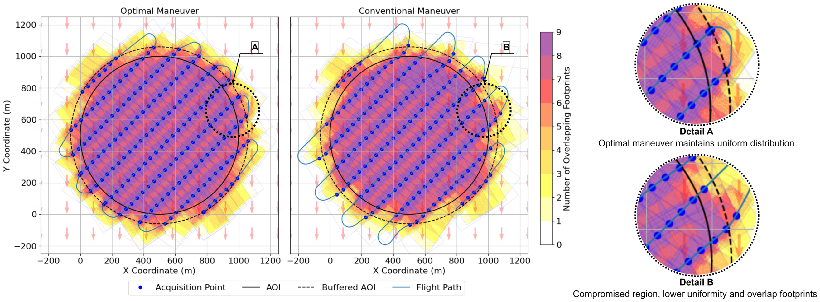
Comparison of image footprints for the optimal and conventional maneuver strategies at a path angle for Test Case 2. Details A and B highlight representative boundary regions: A shows the optimized maneuver, maintaining a more uniform footprint distribution under crabbing, whereas B shows a compromised region with lower uniformity and shifted/overlapping footprints in the conventional strategy.
Figure 25.
Comparison of image footprints for the optimal and conventional maneuver strategies at a path angle for Test Case 2. Details A and B highlight representative boundary regions: A shows the optimized maneuver, maintaining a more uniform footprint distribution under crabbing, whereas B shows a compromised region with lower uniformity and shifted/overlapping footprints in the conventional strategy.
Figure 26.
Comparison of image footprints for the optimal and conventional maneuver strategies at a path angle for Test Case 2. Details highlight the stronger crosswind effect: A illustrates footprint yawing caused by wind-correction crabbing, while B shows the optimized trajectory remaining more consistent with the intended lane-transition direction.
Figure 26.
Comparison of image footprints for the optimal and conventional maneuver strategies at a path angle for Test Case 2. Details highlight the stronger crosswind effect: A illustrates footprint yawing caused by wind-correction crabbing, while B shows the optimized trajectory remaining more consistent with the intended lane-transition direction.
Figure 27.
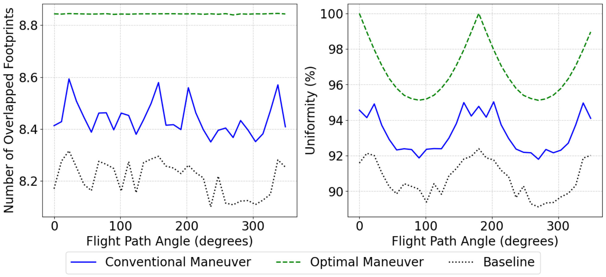
Overlap and uniformity metrics comparison for the optimal and conventional strategies across all path angles for Test Case 2.
Figure 27.
Overlap and uniformity metrics comparison for the optimal and conventional strategies across all path angles for Test Case 2.
Figure 28.
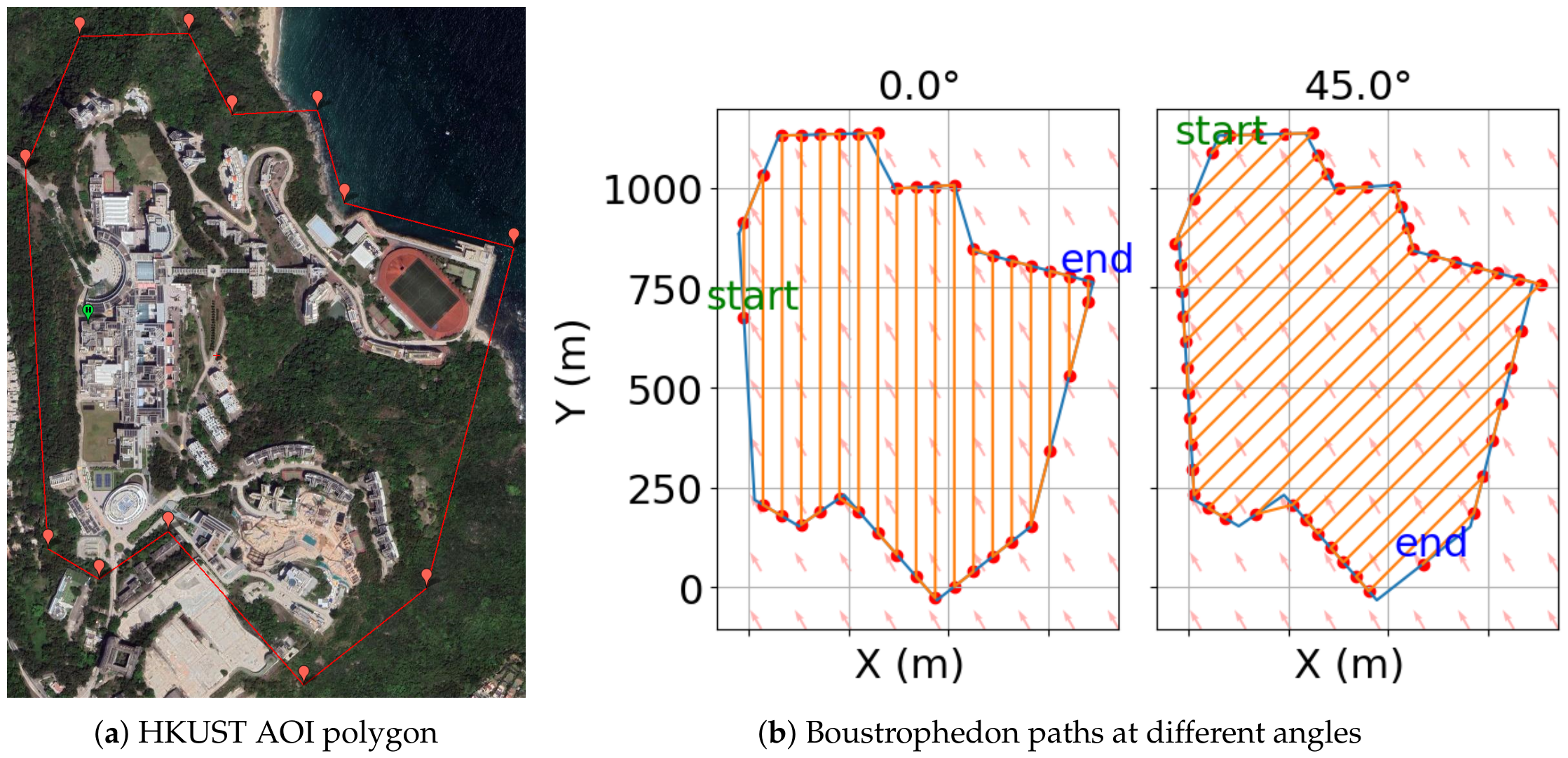
AOI and path setups for Test Case 3.
Figure 28.
AOI and path setups for Test Case 3.
Figure 29.
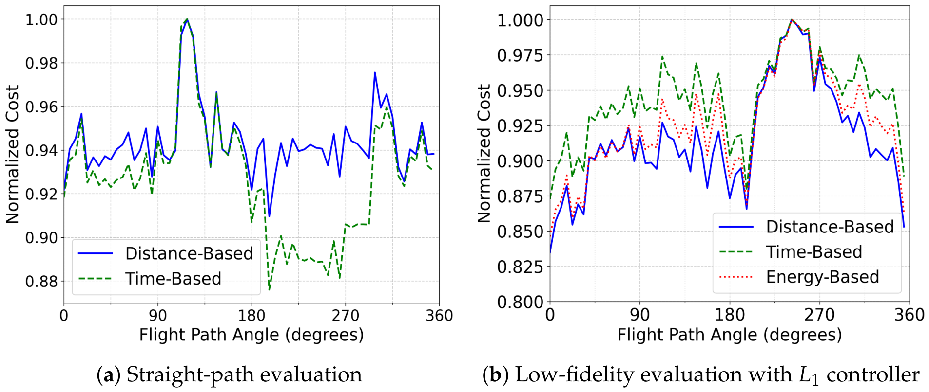
Comparison of cost evaluations for Test Case 3.
Figure 29.
Comparison of cost evaluations for Test Case 3.
Figure 30.
Posterior distribution and acquisition function during BO iterations for Test Case 3.
Figure 30.
Posterior distribution and acquisition function during BO iterations for Test Case 3.
Figure 31.
Comparison between exhaustive evaluation (true function) and BO optimization result for Test Case 3.
Figure 31.
Comparison between exhaustive evaluation (true function) and BO optimization result for Test Case 3.
Figure 32.
Test Case 3 energy-metric comparison over path angle: normalized IEM and relative energy savings of the proposed maneuver strategy versus the conventional baseline.
Figure 32.
Test Case 3 energy-metric comparison over path angle: normalized IEM and relative energy savings of the proposed maneuver strategy versus the conventional baseline.
Figure 33.
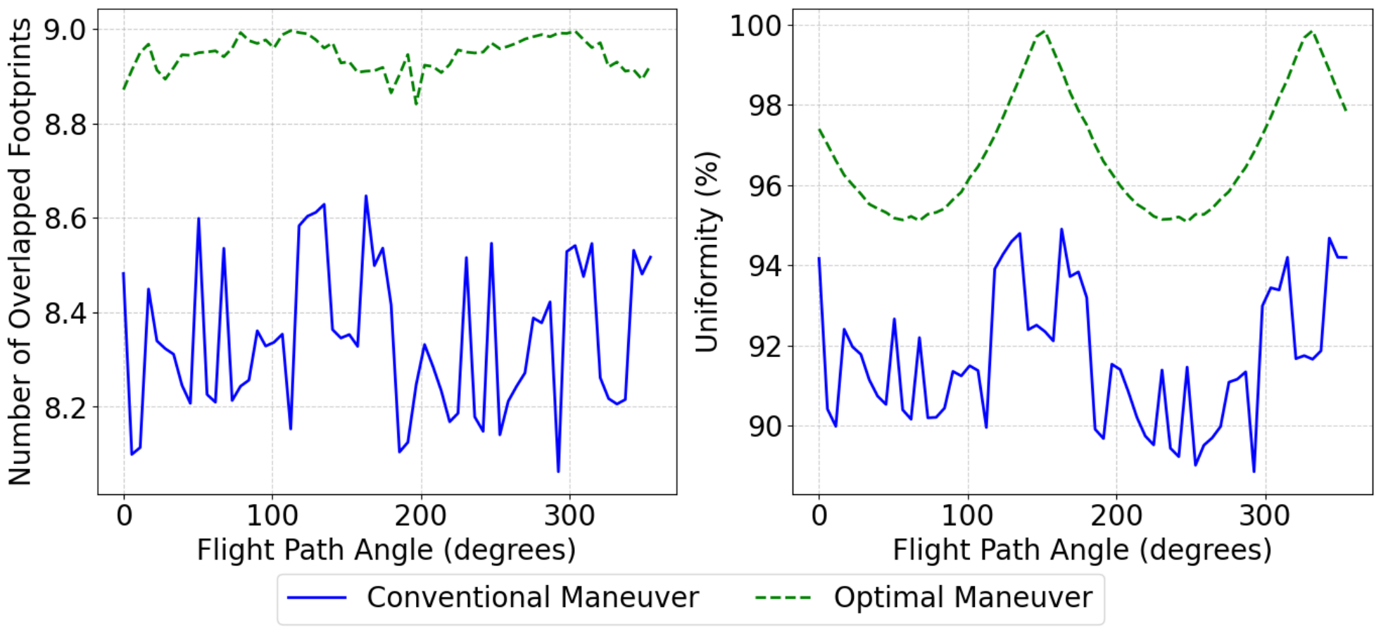
Overlap and uniformity metrics for the optimal and conventional strategies in Test Case 3.
Figure 33.
Overlap and uniformity metrics for the optimal and conventional strategies in Test Case 3.
Figure 34.
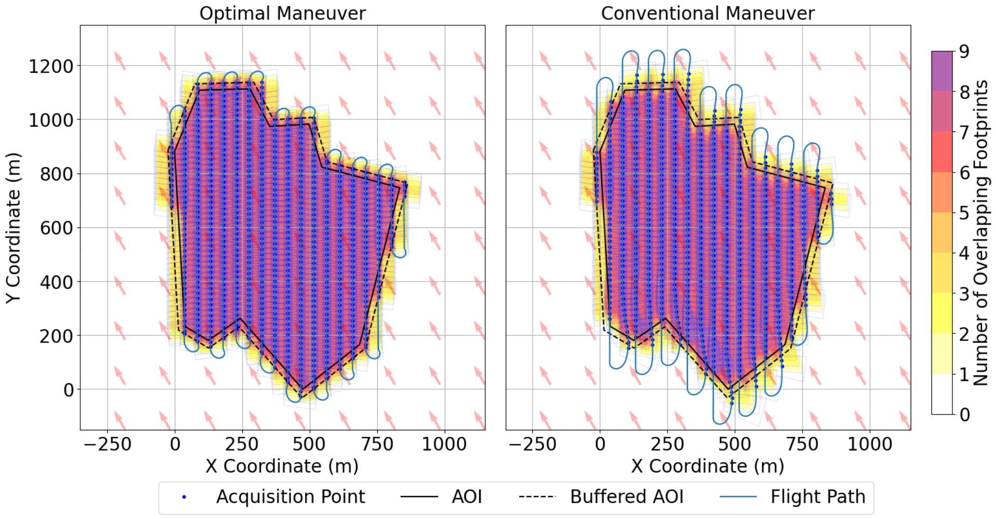
Comparison of footprint distributions for the proposed and conventional maneuver strategies at a path angle for Test Case 3.
Figure 34.
Comparison of footprint distributions for the proposed and conventional maneuver strategies at a path angle for Test Case 3.
Table 1.
Specifications of the BETA Raybe used in the simulations.
Table 1.
Specifications of the BETA Raybe used in the simulations.
| General Parameter | Value |
|---|
| Maximum takeoff weight | 5400 g |
| Wingspan | 1830 mm |
| Length | 1270 mm |
| Wing area | 0.49 |
| Aerodynamic Parameter | Value |
| 0.0210 |
| K | 0.055 |
| 1.25 |
| 16.8 m/s |
Table 2.
Summary of real-flight cases used for trajectory-level simulator comparison. Wind speed and direction were obtained from the aircraft extended Kalman filter (EKF) estimate.
Table 2.
Summary of real-flight cases used for trajectory-level simulator comparison. Wind speed and direction were obtained from the aircraft extended Kalman filter (EKF) estimate.
| Case | EAS | TAS/EAS | TAS | Mean Wind | Wind Dir. | Wind/TAS |
|---|
| | (m/s) | (−) | (m/s) | (m/s) | (° from) | (−) |
|---|
| Light wind | 17.66 | 1.06 | 18.64 | | 320.6 | 0.16 |
| Strong wind | 17.76 | 1.09 | 19.39 | | 79.4 | 0.41 |
Table 3.
Setup conditions for Test Case 2: Basic axisymmetric polygon.
Table 3.
Setup conditions for Test Case 2: Basic axisymmetric polygon.
| Parameter | Value |
|---|
| AOI shape | Axisymmetric polygon (circle-like) |
| AOI radius | 1000 m |
| Wind speed | 5 m/s |
| Wind direction | (from the north) |
| Ground sampling distance (GSD) | 5 cm/pixel |
Table 4.
Setup conditions for Test Case 3: Complex mapping mission at HKUST.
Table 4.
Setup conditions for Test Case 3: Complex mapping mission at HKUST.
| Parameter | Value |
|---|
| AOI shape | Irregular polygon (HKUST campus) |
| Ground sampling distance (GSD) | 2 cm/pixel |
| Wind speed | 5 m/s |
| Wind direction | (southeast) |
Table 5.
Reduction in expensive high-fidelity evaluations achieved by the BO-based workflow relative to exhaustive high-fidelity path-angle sweeps.
Table 5.
Reduction in expensive high-fidelity evaluations achieved by the BO-based workflow relative to exhaustive high-fidelity path-angle sweeps.
| Case | | | | vs. 36 | vs. 72 |
|---|
| Test Case 2 | 17 | 8 | 9 | 52.8% | 76.4% |
| Test Case 3 | 16 | 6 | 10 | 55.6% | 77.8% |