


Highlights
What are the main findings?
- We propose a novel meta-heuristic algorithm, APWMO, with three improvement strategies.
- APWMO outperforms mainstream algorithms in benchmark tests and UAV path planning tasks.
What are the implications of the main findings?
- APWMO provides an effective solution for UAV path planning in complex farmland environments.
- The algorithm and planning framework can be applied to practical agricultural UAV operations.
Abstract
Unmanned aerial vehicle (UAV) path planning is one of the core technologies for realizing precision agricultural operations. In complex farmland environments involving terrain obstacles, tall tree canopies, high-voltage power lines, and restricted no-fly zones, this problem is transformed into a typical multi-objective and multi-constraint optimization problem. Dense constraints drastically narrow the feasible solution space and impose stringent requirements on the convergence, real-time performance, and robustness of planning algorithms. To address this issue, this paper proposes a novel meta-heuristic algorithm: the Agricultural Planting Whole-Cycle Management Optimization (APWMO) algorithm. By integrating the cultivation strategy aligned with crop growth cycle dynamics, the demonstration farmland-based elite guidance mechanism, and the elite archive pruning operation, it achieves a dynamic balance between global exploration and local exploitation. Comparative experiments with 15 advanced meta-heuristic algorithms on the 30-dimensional CEC2017 benchmark test suite show that APWMO achieves the best performance in terms of convergence accuracy, convergence speed, and search stability. Furthermore, the effectiveness of the proposed algorithm is verified in four 3D farmland path planning tasks with different objective weights and complexity levels. Experimental results confirm that APWMO has excellent path planning performance in complex farmland environments and can provide efficient technical support for practical agricultural UAV tasks such as plant protection spraying, crop growth monitoring, and farmland surveying.
1. Introduction
With the rapid iteration of unmanned aerial vehicle (UAV) technology and the continuous advancement of agricultural modernization, UAVs have been widely applied in various farming tasks such as farmland spraying, crop monitoring, and pest and disease control, becoming core equipment for improving agricultural production efficiency and reducing labor costs. As the premise and foundation for UAVs to independently complete farming tasks, path planning, whose rationality and efficiency directly determine the safety, economy, and operation quality of UAV operations, is also a key link connecting UAV technology with practical agricultural applications.
During farming operations, UAV path planning is a core and key issue in the field of UAV applications, aiming to plan a safe and efficient flight path from the starting point to the target point for UAVs performing tasks. It not only needs to accurately avoid airspace hazards such as terrain obstacles, no-fly zones, severe weather, and tall structural barriers (e.g., power lines and tree canopies) and strictly meet its own physical constraints such as maneuverability and turning radius but also coordinately optimize multiple conflicting performance objectives [1,2]; especially in complex agricultural environments such as mountainous areas and dense orchard areas, 3D path planning presents characteristics of strong nonlinearity, high dimensionality, and multiple constraints, putting extremely high requirements on the real-time performance, robustness, and global optimization ability of the algorithm [3]. Single-UAV path planning focuses on generating the optimal or shortest path for a single UAV in a designated agricultural operation area, ensuring the smooth execution of tasks such as spraying, crop monitoring, and agricultural surveying, while minimizing flight time and energy consumption. In contrast, multi-UAV collaborative path planning needs to achieve efficient coordination between formations. While completing the independent planning of each UAV, it also solves problems such as conflict avoidance, collaborative operation, and task coordination. It is necessary to improve the operation efficiency and safety of a single UAV and also take into account task allocation, inter-UAV interference suppression, and overall operation efficiency optimization. How to meet collaborative constraints on the premise of ensuring the independent planning of each UAV has become the focus and difficulty of current research.
Under dynamic farmland and complex airspace conditions, the motion modeling and path planning of UAVs face greater uncertainty. Existing studies have attempted to construct the motion state of UAVs as a Markov process [4] and deduce the current spatial position through state quantities such as position and speed at the previous moment, realizing a time–space coupled state description, which gives it significant advantages in dealing with scenarios such as dynamic obstacles and sudden hazards. At the same time, traditional ideas also try to add supervision and constraint modules to the single-UAV path planning framework to meet the safety and compliance requirements of multi-UAV collaboration. However, such methods generally have limitations such as large computational overhead, insufficient real-time performance, and weak scalability, making it difficult to adapt to large-scale multi-UAV collaborative scenarios.
Therefore, a growing number of studies have shifted to intelligent optimization algorithms, using the idea of multi-population cooperative optimization to address multi-UAV path planning problems [5]. Centered on population-based iterative optimization, these methods can efficiently search for feasible solutions in high-dimensional, non-convex, and highly constrained solution spaces, providing a more practical technical approach for cooperative trajectory generation of multiple UAVs.
Regarding path planning methods, existing solutions can be roughly divided into five categories: graph-based methods, sampling-based methods, artificial potential field methods, reinforcement learning methods, and swarm intelligence algorithms.
At present, UAV path planning methods have formed a diversified technical system, and various approaches show distinct performance differences and applicable boundaries in complex farmland environments. Early studies mostly relied on mathematical programming methods (e.g., mixed-integer linear programming, dynamic programming, etc.) [6,7,8]. Although these methods can obtain theoretically optimal solutions in low-dimensional scenarios, they suffer from computational explosion and fail to meet real-time requirements when facing three-dimensional, highly constrained, and large-scale cooperative missions. Graph-search methods represented by the Dijkstra and A* algorithms [9,10] are widely used in two-dimensional planning due to path optimality, but their search efficiency drops sharply in high-dimensional complex airspace. Sampling-based methods (PRM and RRT series) [11,12] do not require precise environment modeling and can quickly generate feasible trajectories with strong adaptability to motion constraints and multi-degree-of-freedom problems. However, they commonly have shortcomings such as insufficient path smoothness and lack of guaranteed optimality. The artificial potential field method [13,14] features a simple structure and high real-time performance but easily falls into local optima and exhibits poor stability in threat-dense complex environments. Reinforcement learning [15,16] autonomously learns decision-making strategies through agent–environment interaction and reward mechanisms, showing potential in dynamic confrontation scenarios. Nevertheless, it relies on extensive trial-and-error training, and its model generalization ability and convergence stability still need improvement.
Precisely because traditional methods have limitations in high-dimensional, highly constrained, and dynamically cooperative scenarios, swarm intelligence and meta-heuristic algorithms have gradually become the mainstream technical route. Various heuristic algorithms including the Genetic Algorithm (GA) (Holland, 1992), Particle Swarm Optimization (PSO) (Kennedy and Eberhart, 1995), Ant Colony Optimization (ACO) (Dorigo et al., 1996), and Harris Hawks Optimization (HHO) (Heidari et al., 2019) [17,18,19] have been widely applied to real-time UAV path planning owing to their simple structure, strong optimization ability, and wide adaptability. They can output flyable trajectories that meet maneuvering, obstacle avoidance, and coordination requirements within a limited time. However, single algorithms vary significantly in performance under different constraints and scenarios, which has driven the academic community to continuously propose improved strategies and novel intelligent optimization methods. Against this background, the idea of multi-population cooperative optimization has been introduced into multi-UAV path planning. Relying on the population iterative optimization mechanism, it provides more stable search ability in high-dimensional, non-convex, and highly constrained solution spaces, offering a more engineering-practical solution for real-time cooperative trajectory generation of multiple UAVs.
In recent years, numerous improved strategies and novel intelligent optimization methods have emerged: Niu et al. [20] proposed a path planning method based on continuous Ant Colony Optimization, which effectively improves the efficiency and accuracy of three-dimensional path planning by integrating improved state transition probability, random walk, and adaptive trajectory point modification strategies. The Gray Wolf Optimizer and its improved variants have also been applied to solve this problem with satisfactory results [21]. Han et al. [22] improved the Artificial Bee Colony algorithm using multiple strategies and applied it to helicopter path planning. Simulation results verified the algorithm’s significant advantages in fuel economy and flight safety. Van et al. [23] proposed a Fermat–Weber Location-based Particle Swarm Optimization (FWL-PSO) algorithm for UAV path optimization. This method effectively enhances the learning mechanism of standard PSO, promoting search diversity while achieving information co-evolution. Liu et al. [24] applied the Crested Porcupine Optimizer (CPO) to UAV path planning in complex environments and achieved favorable performance. Inspired by the natural behavior of graylag geese, El-Kenawy et al. [25] proposed the Graylag Goose Optimization (GGO) algorithm. Qualitative analysis and validation experiments confirmed its superior performance in handling UAV path optimization problems. To address the tendency of UAV three-dimensional path planning to fall into local optima, Zhou et al. [26] proposed an improved Pelican Optimization Algorithm (LPOA) integrating predator–prey strategy and Levy flight. The algorithm enhances global optimization and convergence speed through chaotic initialization, adaptive parameter updating, and enhanced prey generation strategies. Experimental results show that the algorithm can optimize the total objective cost by 9.75% and the average shortest path by 20.30%. Qi et al. [27] proposed a path planning method based on an improved Non-dominated Sorting Genetic Algorithm III (NSGA-III). Based on establishing a mathematical model for simultaneous arrival, a multi-objective trajectory generation framework integrating time coordination, threat avoidance, and resource consumption was constructed. The NSGA-III was improved by fusing the Artificial Bee Colony (ABC) algorithm to enhance search accuracy and convergence speed under complex constraints. Simulation results demonstrate that the method can optimize flight time, reduce resource consumption, and strengthen threat avoidance while ensuring simultaneous arrival of UAV clusters. Li et al. [28] proposed a guided cooperative control mechanism forming a novel multi-UAV cooperative path planning method. An improved Multi-Dimensional Coati Optimization Algorithm (MDCOA) was developed by introducing Levy flight, differential operator, dynamic opposition-based learning, and Covariance Matrix Learning (CML) for path solution. Experimental results in various offshore simulation scenarios show that the paths obtained by the algorithm effectively reduce path cost and outperform other comparison algorithms, verifying the effectiveness and scalability of the proposed method. In addition to the above examples, recent novel meta-heuristic algorithms such as CPO [29] (Crested Porcupine Optimizer, Guo et al., 2025), TOC [30] (Tornado Optimizer with Coriolis Force, Malik et al., 2025), CJADE [31] (Constrained Joint Adaptive Differential Evolution, Gao, 2019), ESC [32] (Escape Optimization Algorithm, Ouyang et al., 2024), CSA [32] (Chameleon Swarm Algorithm, Malik et al., 2021), BKA [33] (Bat King Algorithm, Wang et al., 2024), CPSOGSA [34] (Constricted Particle Swarm Optimization Gravitational Search Algorithm, Rather, 2020), and IAO [35] (Information Acquisition Optimizer, Wu et al., 2024) have all shown great potential in UAV path planning.
However, existing studies indicate that UAV path planning is highly complex and scenario dependent, and no single algorithm can achieve universal applicability and optimal performance across all scenarios. Therefore, developing more efficient and robust intelligent optimization methods remains a core research hotspot in this field. Furthermore, publicly available applications and validation cases of recent novel intelligent optimization algorithms in agricultural operational scenarios are relatively scarce. UAV path planning methods for complex farmland environments urgently require further breakthroughs and improvements.
To address the UAV path planning problem, this paper proposes the Agricultural Planting Whole-Cycle Management Optimization Algorithm (APWMO). This algorithm finds optimal solutions by simulating the whole-process management logic of farmers from “field planning to crop harvesting” [36]. Its core idea is to convert the “optimization objective” of the algorithm into the “quality of crop growth” and map each “candidate solution” to an “independent planting unit”. By replicating the wisdom of agricultural production—dynamic adjustment with growth stages, avoiding repetition via experience, and controlling boundaries to prevent risks—the algorithm balances global exploration and local search and finally converges to the optimal scheme. This meta-heuristic algorithm is designed to plan feasible flight paths for fixed-wing UAVs. The main contributions of this paper are as follows:
- (1)
- A virtual operational environment incorporating elements such as terrain obstacles, tall tree canopies, and high-voltage power lines is constructed. Based on the number and distribution of obstacles, four test tasks with different objective weights and complexity levels (Task 1 to Task 4) are designed.
- (2)
- For UAV path planning in complex environments, the APWMO algorithm is proposed. The algorithm introduces three strategies: a planting strategy matching crop growth cycles, a “demonstration farmland” strategy, and an elite archive pruning mechanism. The performance of APWMO is verified on 30-dimensional problems from the CEC2017 benchmark, and a rigorous comparative analysis with 15 other advanced intelligent algorithms shows that APWMO ranks first.
- (3)
- The proposed algorithm is validated through experiments. The results demonstrate that the APWMO algorithm can find optimal or near-optimal flight paths for UAVs. Comparative experiments confirm that the APWMO algorithm outperforms other existing algorithms in multi-UAV path planning tasks in complex environments.
The technical route of this paper is as shown in Figure 1. The specific methods for each stage are as follows:
Figure 1.
The technical route adopted in this research.
First, this paper clearly defines the core connotation of the UAV path planning problem and systematically introduces various constraints encountered in the planning process, such as UAV maneuverability constraints and farmland obstacle constraints, laying a theoretical foundation for subsequent algorithm design and verification.
Then, this paper elaborates on the three core strategies of the APWMO algorithm, namely the cultivation strategy combined with crop growth cycle matching, demonstration farmland strategy, and elite archived pruning mechanism. The design logic and implementation details of each strategy are clearly explained, along with their key roles in the algorithm’s optimization process.
Next, comprehensive tests and analyses are conducted on the performance of the APWMO algorithm using the CEC 2017 benchmark suite. By comparing it with 15 state-of-the-art meta-heuristic algorithms, the superiority of the proposed algorithm in key indicators such as optimization accuracy and convergence speed is verified.
Finally, the APWMO algorithm and eight high-performing algorithms from the CEC2017 test suite are applied to the multi-UAV three-dimensional path planning problem. Through multi-scenario simulations, the path planning performance of all comparative algorithms in complex farmland environments is comprehensively evaluated, further validating the engineering practicability of the APWMO algorithm.
2. UAV Trajectory Planning Scene Model Construction
2.1. Description of the Trajectory Planning Problem
This study is set to conduct research on multi-UAV trajectory planning in a known environment, an example of which is shown in the Figure 2. To clearly describe the motion scene, the absolute Cartesian coordinate system is adopted for the description and modeling below.
Figure 2.
Schematic diagram of the obstacles encountered by the unmanned aerial vehicle during flight.
Compared with the obstacle avoidance and cost factors such as flight turning, height, and length that need to be considered in single-UAV path planning, “avoiding inter-UAV collisions” is an additional key issue that needs to be focused on solving in the multi-UAV collaborative operation scenario. Therefore, the core objective of this problem is as follows: under the premise that the starting positions, target positions, environmental elements, and obstacle distribution are all fixed, guide multiple UAVs to fly to their respective target positions, and minimize the overall flight cost while avoiding inter-UAV collisions and environmental obstacles.
Among them, the environmental obstacles include tall tree canopies, high-voltage power lines, and no-fly zones, and their specific representations are shown in the Figure 2 below:
- (1)
- The starting point and target point are defined as S and G, respectively.
- (2)
- Tall tree canopies are marked with green dashed circles, and high-voltage power lines are marked with red dashed circles. Both types of dashed circles represent dangerous areas where “UAVs have a certain probability of collision”, and UAVs will not be at risk of collision after leaving these areas.
- (3)
- No-fly zones are represented by red dashed rectangles, and UAVs are strictly prohibited from flying into these areas (such as agricultural facility protection areas and farmland operation areas with dense personnel activities).
In the process of path optimization, three types of costs need to be minimized simultaneously: flight length cost, flight height cost, and collision cost from tall obstacles and low-altitude interference sources; at the same time, three constraints need to be satisfied: yaw angle constraint, climb angle constraint, and no-fly zone avoidance constraint.
2.2. Path Representation and Smoothing
2.2.1. Path Representation
In the research of this paper, it is assumed that the flight speed of the unmanned aerial vehicle is fixed and that the location of the threat area is known. Each unmanned aerial vehicle is equipped with a track control point. The route of each UAV consists of the starting position S, the destination position G, and N-2 route points between S and G, which are evenly distributed. The coordinates of the path point j of unmanned aerial vehicle i are:
Among them, the value range of i is from 1 to I, and the value range of j is from 1 to N-2.
I represents the total number of unmanned aircraft. From this, it can be known that the complete path of unmanned aerial vehicle i can be expressed as: .
2.2.2. Path Smoothing
During the planning process, the flight path of the unmanned aerial vehicle consists of N to 2 waypoints. In fact, path planning is the optimization of the positions of waypoints. However, due to the physical constraints of fixed-wing unmanned aerial vehicles, the planned flight path cannot meet the flyable conditions. Therefore, it is necessary to introduce a feasible smoothing strategy. This paper introduces the B-spline [37] curve method for the smoothed optimal path, which is widely used in path smoothing problems.
Suppose the path to be optimized for a certain unmanned aerial vehicle is Pi; then, the B-spline curve method is composed of Pi, B-spline basis functions Ni,k(u), and node vectors U = [u0,u1,…,um], and the curve equation is expressed as follows:
The basis function Ni,k(u) is updated by the de Cox–Boor equation, Equation (3) (where k is the order).
2.3. Model for Unmanned Aerial Vehicle Trajectory Planning Problem
Unmanned aerial vehicle trajectory planning is a complex optimization problem with multiple constraints and objectives. The modeling of this article is as follows.
2.3.1. Threat Cost
Different from the strict no-fly zone hard constraint, the collision constraints of tall tree canopies and high-voltage power lines are defined as soft constraints. For such soft constraints, UAVs are permitted to enter the surrounding influence area of obstacles, but corresponding collision penalty costs will be imposed once the UAV flies into the affected range. The closer the UAV approaches the obstacle center, the higher the collision risk and the greater the penalty cost.
Both tall tree canopies and high-voltage power lines are major collision obstacles in UAV agricultural operations. Among them, the collision probability of tall tree canopy obstacles depends on the distance between the UAV’s waypoint and the center of the tree canopy, whose center coordinates are (xR,yR,zR), is the maximum influence radius, and k is the collision risk degree, and the closer the UAV is to the center of the tree canopy, the greater the collision risk; FCanopy is used to represent its collision cost. High-voltage power line obstacles will put UAVs within their influence range at risk of collision, da is the distance between the UAV and the center of the high-voltage power lines, and Ra is the maximum influence radius, and the closer the UAV is to the high-voltage power lines, the greater the collision danger; FLine is used to represent its collision cost, and the relevant formulas are as follows:
2.3.2. Length Cost and Height Cost
- (1)
- Length cost
Length cost refers to the length of the flight path of a drone. Under the condition of a constant flight speed, the shorter the path distance, the less energy the drone consumes. Therefore, a shorter path is preferred. The ratio is typically used to represent the cost of path length, and the corresponding function can be calculated as follows:
Here, li represents the distance from track point i to i + 1; is the Euclidean distance from the starting point S to the target point G.
- (2)
- High cost
To ensure the safer flight of drones, their flight altitude should not be too high. At the same time, the drone should not be too low either. It is usually between two given extreme values, namely the maximum altitude and the minimum altitude. Take aerial reconnaissance as an example. The cameras carried by UAVs need to meet specific resolution and field-of-view requirements to satisfy the demands of data collection. Therefore, restrictions on flight altitude are necessary. The high cost is expressed as follows:
In the formula, hmin and hmax represent the minimum and maximum flight altitudes, respectively. hi is the flight altitude of the unmanned aerial vehicle at track point i. In the formula, penalties are imposed for exceeding the upper and lower extreme values of the flight altitude, thereby enabling the average altitude to be maintained.
2.3.3. Single-Machine Constraint Processing
The collaborative airway of multiple unmanned aerial vehicles must, on the one hand, meet the physical performance constraints of a single UAV itself and, on the other hand, comply with the requirements of collaborative constraints among multiple UAVs. This paper will adopt the penalty function approach to handle various constraints of UAVs. In this section, the focus is on elaborating the handling of single-UAV constraints:
- (1)
- Maximum yaw angle
The maximum yaw angle of a drone refers to the maximum angle at which the projection of its flight path on a horizontal plane changes. Due to the constraints of its own performance and inertia, if a UAV needs to change its flight direction during flight, it can only turn within the maximum yaw angle range and cannot travel at any angle. The imposed constraints and the formula for the yaw angle are shown in Equation (38), where represents the offset angle of the current track line segment relative to the previous track segment.
- (2)
- Maximum pitch angle
The maximum pitch angle of a drone refers to the maximum angle between the drone’s axis and the horizontal plane during its ascent or descent. Due to the performance constraints of the UAV itself and for safety and speed control, if it needs to climb or descend during flight, the angle must be less than the maximum pitch angle. The constraints applied in the text and the formula for the pitch angle are shown in Equation (8), where is the pitch angle of the current route corresponding to the previous route.
- (3)
- Minimum track segment constraint
During the flight of an UAV, there is a stable process of changing from one attitude to another. This stable flight path is called the minimum straight-line flight path distance. At the same time, apart from the limitations of the UAV’s own functions, due to the communication delay between the UAV and the ground control center, the straight-line flight distance during the delay period must also be taken into account when flying at high speed. Therefore, ensuring the minimum flight path segment in the process of UAV flight path planning is an important prerequisite for planning a reasonable flight path. Let the distance of the minimum track segment caused by the functional limitations of the UAV and the maximum delay be Lmin. Therefore, the constraints imposed on the distance of any straight track in the track are as follows:
- (4)
- No-fly zone restrictions
UAVs need to avoid flying into clearly defined areas, such as some sensitive regions, and also stay away from high-voltage lines, high-rise buildings, crowded places, etc. The definition of the no-fly zone constraint NFZ is as follows:
Here, and are the lower and upper limits of NFZ in the x-coordinate, while and are the lower and upper limits in the y-coordinate.
UAVs are required to bypass predefined restricted areas including sensitive regions, high-voltage lines, high-rise buildings, and crowded areas.
2.3.4. Multi-Machine Collaborative Constraints
In multi-UAV path planning, not only the obstacle avoidance issue needs to be considered but also the coordination relationships need to be handled, including spatial coordination and temporal coordination.
- (1)
- Time coordination constraints
The so-called time coordination refers to the fact that when a multi-UAV system is performing a mission, the time when each aircraft reaches the target point should satisfy a certain specific relationship. This paper mainly studies the simultaneous arrival of each aircraft at the target point. In real scenarios, the speed of drones varies within a certain range, and the time it takes for them to reach the target point cannot be exactly the same. Therefore, as long as the time ranges for each UAV to reach the target point overlap, it can be considered that all UAVs can reach the target point simultaneously.
The time coordination set in this paper is as follows: Let the instruction time for the UAV to reach the target endpoint be tc, and ensure the time coordination of the UAV through the instruction time constraint. The time range [tmin,tmax] for the UAV to reach its destination can be obtained from the speed range and track length of the UAV, that is:
Among them, and are the time range when the i-th UAV reaches its destination; L and v represent time and speed, respectively.
If it is , it can be regarded as achieving formation coordination.
Finally, the (time cost) is obtained as:
- (2)
- Spatial collaborative constraints
To ensure that multiple UAVs are not at risk of colliding with each other, it is necessary to test whether they are too close to each other when traveling along the paths planned for them. For this purpose, it is necessary to compare the node coordinates on the planned paths of multiple UAVs with each other. If the distance between UAVs at the same time is less than the safe distance, there is a risk of scraping.
Among them, represents the distance between the track point i of the UAV and other UAVs at the same time. is the safe distance for the unmanned aerial vehicle.
2.3.5. Spherical Vector Coordinate Frame
To improve the feasibility and smoothness of path solutions, this paper adopts the idea from Ref. [38] and uses a spherical vector coordinate system to encode the segment motion of UAVs.
Taking the current waypoint as the local origin, the spherical vector coordinate system uses three parameters to describe the position of the next waypoint: the radial distance r (Euclidean distance between two waypoints), the polar angle (the angle between the segment vector and the z-axis, corresponding to the pitch direction), and the azimuth angle (the angle between the projection of the segment vector on the xOy plane and the x-axis, corresponding to the horizontal turning direction). The conversion relationship with Cartesian coordinates is:
where is the coordinate of the current waypoint, and is the coordinate of the next waypoint.
The spherical vector encoding generates segment parameters based on the previous waypoint, which naturally ensures the continuity of the waypoint sequence and avoids trajectory mutations. Its polar angle and azimuth angle directly correspond to the pitch angle and turning angle of the UAV, making it convenient to apply kinematic constraints during the encoding stage and significantly improving the probability of generating feasible solutions. Meanwhile, in scenarios with fixed flight speed, the problem dimensionality can be simplified by fixing the radial distance , focusing on optimizing the angular parameters to reduce the search complexity of the algorithm.
2.3.6. Objective Function
In this paper, the linear weighted sum method is adopted to transform the constraints into objectives for path planning. This method is usually used to handle practical optimization problems. The entire objective function is regarded as the evaluation function of the candidate path.
The objective function of this paper consists of threat cost, length cost, altitude cost, maximum yaw constraint, maximum pitch angle constraint, minimum track segment constraint, no-fly zone constraint, temporal coordination constraint, and spatial coordination constraint. Among them, the constraint conditions are added to the objective function in the form of penalty functions, and the mathematical expression of the objective function is as follows:
where w denotes the weight vector. In this paper, three groups of differentiated weight vectors are set to carry out weight sensitivity analysis, which focus on three task preferences, respectively: threat avoidance, maximum flight range, and temporal–spatial collaboration constraint. The influence law of each sub-objective weight coefficient on the optimal trajectory and comprehensive objective function of multi-UAV path planning is explored. The detailed settings are as follows:
3. Core Algorithm Strategy
3.1. Physical Background and Sources of Inspiration
In modern agricultural production [39,40], it is necessary to dynamically adjust field management measures such as irrigation, fertilization, and pest and disease prevention and control at each growth stage of crops, including the seedling stage, jointing stage, and grain filling stage. In addition, farmers learn from each other’s planting experience, which leads to differentiation in management schemes among different planting units and obvious differences in yield performance.
The algorithm candidate solutions are mapped to crop planting management schemes, and the solution space is composed of controllable agricultural variables such as fertilizer application amount, irrigation water volume, and planting density. Each scheme can learn from the variable proportion relationships of others and explore brand-new variable combinations through trial and error. Under the balance of experience reuse and unknown region search, it gradually converges to the optimal high-yield management scheme.
The crop growth cycle adaptive farming strategy, demonstration farmland strategy, and elite archive pruning mechanism are the three core strategies to guarantee the optimization performance.
3.2. Cultivation Strategy Combined with Crop Growth Cycle Matching
3.2.1. Initial Population and Parameter Settings
Before engaging in agricultural cultivation, it is first necessary to divide the farmland into N equally large “planting units” (population sizes), which are managed by different farmers.
The specific operation is as follows: In the D-dimensional search space, first set the population matrix . The lower and upper bound of the population are, respectively, represented as and . Here, in the field, the physical meaning represents the degree of watering, fertilizing, loosening the soil, etc., where d represents the dimension.
In , the cultivation strategy (initial position) and growth condition (fitness) of each “planting unit” are defined by the following formulas (Equations (16) and (17)):
3.2.2. The Choice of Farmers’ Attitudes and the Extent of Reference
Taking rice as an example [41], crop growth is divided into the seedling stage, jointing stage, and grain filling stage. The growth cycle coefficient is defined as formula (18), where is the current iteration step, and maxFES is the maximum iteration step of the whole cycle. The larger is, the smaller is, indicating that the crop is more mature (Figure 3).
Figure 3.
CF(t) variation with t (maxFES = 10,000).
The strategy attitude coefficient is defined as Equation (19), corresponding to the planting attitude of farmers. Farmers extensively learn from others and conduct trial and error, resulting in high population diversity and making the algorithm not easy to fall into the local optimum.
The reference amplitude is defined as Equation (21) (including scaling factor), where is the scaling factor:
This index characterizes the learning penetration intensity and behavior adjustment step size of farmers’ learning and imitating production decisions from other individuals. Equation (22) constrains it to be non-negative. decreases nonlinearly in [0, 1] with random perturbation. It adopts an adaptive strategy of dynamic base value coupled with iteration progress plus Cauchy distribution perturbation, taking into account the stability of core search step size and the randomness of global exploration.
3.3. Demonstration Farmland Strategy
3.3.1. Selection of “Demonstration Farmland”
During the process of cultivation, some outstanding farmlands emerged, which can provide good references for other farmlands.
To accelerate the optimization process, we select the current optimal p planting units (with an elite ratio rp set in this article) to form “demonstration farmland” . The relevant formulas are as follows:
These “demonstration farmlands” represent the high-quality solutions in the current search space. Each planting unit should randomly select a planting unit from the “demonstration farmland” as its reference farmland to push it towards a better solution. This process is similar to borrowing information from excellent solutions during the optimization process to accelerate convergence. The specific operation is to first generate N random integer vectors k, where each element , as shown in (25):
Subsequently, for each solution j, the corresponding optimal solution is selected from the “demonstration farmland” by random index kj to form the reference elite matrix :
Among them, , and represents the high-quality solution with index in the original population.
3.3.2. Generation of “New Farming Strategies”
Of course, farmers naturally hope that their farmland grows best. If they only rely on their own exploration, it will be a long process. At this time, the guidance of agricultural experts is indispensable.
The expert combined the current scheme set Xt adopted by all planting units and the historical cultivation scheme At (where A is an empty set before the algorithm iteration) into a full scheme library S, as shown in Equation (27):
Agricultural experts randomly sorted (randomly permutation index) the indexes of the “population scheme library” Xt and the “total scheme library” St through the LHS method, obtaining Equations (28) and (29), which, respectively, represent the indexes of the “population scheme library” and the “total scheme library”:
Take the top N of the population scheme library to obtain:
Subsequently, the experts selected one household each from the “population scheme library” Xt and the “full scheme library” St for research, which were, respectively, denoted as and , among which:
Define the difference matrix:
On this basis, experts generate new farming strategies by combining current experience with historical experience to ensure the effectiveness of the exploration. This difference represents the phase difference between understandings. Through the guidance of the difference matrix, we can generate new farming strategies. The generation formula of the new farming strategy Xnew is as follows:
3.4. Elite Archived Pruning Mechanism
3.4.1. Boundary Control
New farming strategies sometimes encounter extremely unreasonable situations (corresponding solutions exceed the predetermined search space boundaries). To avoid this situation from happening, we adopted the following method (boundary processing approach). When the component of a certain solution exceeds the boundary, we fine-tune it to the legal region. Specifically, the conditions for adjustment are as follows:
3.4.2. Compulsory Learning Strategy
Agricultural experts, in order to ensure better growth of crops, enforce that every household must learn at least one farming strategy from other households. Among them, one strategy that each household must learn is represented by a random dimension index, as shown in Equation (36):
Farmers, on the other hand, decide whether to learn from other farmers based on their attitude coefficient α towards the new farming strategy. Here, a logical mask matrix is constructed, where:
Subsequently, a new cross-solution was obtained as shown in the following formula:
3.4.3. Evaluation and Selection and “Elite Archive Trimming”
At this point, the growth of cultivated land after adopting the new strategy is evaluated. The new fitness is denoted as , and the specific calculation formula is as follows:
If the growth condition of the crops is better than that of the original crops after adopting the new strategy at this time, then replace the original plan with the new one:
At the same time, store the replaced “old plan” in the historical archive At+1. The specific operation is as follows:
If At+1 > N, sort the archive in ascending fitness order, and only retain the first N optimal solutions (j1–jN are the first N indexes after sorting):
At regular intervals, identify the best-growing scheme xtbest and the growth conditions ftbest of the corresponding yield planting units, and record them. The algorithm ends when the total duration of the entire planting cycle is reached.
3.5. Pseudo-Code
The complete step-by-step process of APWMO is listed in Algorithm A1. This pseudo-code outlines the core stage of its algorithm.
3.6. Complexity Analysis
The complexity of swarm intelligence optimization algorithms mainly depends on the population size N, problem dimension D, fitness function C, and maximum number of iterations T. In a single iteration of the algorithm, the fitness function is evaluated N times to measure the algorithm performance, resulting in a total of NT function evaluations during execution.
For the APWMO algorithm, its complexity consists of two parts: initialization and iterative loop. In the initialization phase, population individuals are randomly generated, and their fitness values are evaluated. The complexity of random individual generation is O(ND), and the complexity of fitness calculation for the initial population is O(NC). Thus, the overall complexity of the initialization phase of APWMO is O(ND + NC). During the iterative loop of APWMO, the main operations include population position updating, fitness evaluation, external archive maintenance, and sorting, with computational complexities of O(TND), O(TNC), and O(TNlogN), respectively. Therefore, the overall time complexity of the APWMO algorithm can be expressed as:
4. Basic Verification of Algorithm Performance
4.1. Experimental Setup
To verify the effectiveness of the proposed strategy and evaluate the overall performance of the APWMO algorithm, simulation experiments are conducted on the CEC2017 [42] test set. The CEC2017 benchmark function set contains 29 test functions, among which F2 is removed due to unstable performance. These functions are divided into four categories: unimodal functions (F1 and F3), simple multimodal functions (F4–F10), hybrid functions (F11–F20), and composite functions (F21–F30). In the subsequent experiments, the dimension D of all test functions is set to 30. The serial number, function description, value range, and theoretical minimum value of the test functions are listed in Table 1. Comparative experiments are carried out between the APWMO algorithm and 15 other state-of-the-art intelligent algorithms.
Table 1.
Test functions of CEC2017.
The performance superiority of the proposed algorithm is verified by comparing with a variety of classic and mainstream intelligent optimization algorithms, including PSO (Particle Swarm Optimization) [43] (Kennedy, 1995), EDBO (Improved Differential Evolution-Based Optimization) [44] (Xue, 2022), STOA (Sooty Tern Optimization Algorithm) [45] (Dhiman, 2019), GWO (Gray Wolf Optimizer) [46] (Mirjalili, 2014), AO (Aquila Optimizer) [47] (Abualigah, 2021), SFOA (Sparrow Flight Optimization Algorithm) [48] (Zhong et al., 2025), SCA (Sine Cosine Algorithm) [49] (Mirjalili, 2016), DE (Differential Evolution) [50] (Storn, 1997), WOA (Whale Optimization Algorithm) [51] (Mirjalili, 2016), CSA (Capuchin Search Algorithm) [52] (Braik, 2021), MTDE (Multi-Trial Differential Evolution) [53], THRO (Tianji’s Horse Racing Optimization) [54] (Wang et al., 2025), HHO (Harris Hawks Optimization) [55] (Heidari et al., 2019), AOA (Arithmetic Optimization Algorithm) [56] (Abualigah et al., 2021), and BKA (Black-winged Kite Algorithm) [33] (Wang et al., 2024).
Among them, DE and MTDE are high-performance optimization algorithms; PSO, GWO, the WOA, AO, SCA, and CSA are widely cited mainstream algorithms; and the SFOA, STOA, EDBO, THRO, BKA, HHO, and AOA are popular and widely concerned meta-heuristic algorithms. Therefore, these 15 excellent intelligent algorithms are selected as comparison algorithms to evaluate the performance of APWMO. The parameter settings of all algorithms adopt the recommended configurations in their original literature, as shown in Table 2.
Table 2.
Parameter configuration of the algorithm.
In terms of the selection of evaluation indicators, the final statistical indicators include the mean (mean), standard deviation (standard deviation, abbreviated as Std) and average runtime (average runtime, abbreviated as T) of each algorithm. To conduct a statistical analysis of the significant differences in algorithm performance, the Wilcoxon rank-sum test was adopted, with the significance level set at 0.05. To clearly present the results, this paper uses “+”, “=“, and “−” to, respectively, indicate that the performance of the APWMO algorithm is better than, equal to, or worse than that of each comparison algorithm.
In all the experimental tests of this study, the population size N of all algorithms was set to 200, and the maximum number of iterations was set to 3000. To ensure the reliability of the results, each algorithm was independently run 30 times on the MATLAB (R2020b) platform. The hardware environment for the operation of the experimental program is a personal computer with a Windows 11 system, configured with an Intel Xeon(R) CPU E5-2689 v4@3.10GHZ processor (main frequency 3.10 GHz) and 96.0 GB of memory.
4.2. Convergence Analysis
The core theoretical basis of this proof is the well-recognized Solis–Wets global convergence theorem in the field of stochastic optimization [57]. The theorem gives the necessary and sufficient conditions for stochastic search algorithms to converge to the global optimal solution in probability, and the original statement is as follows:
Theorem 1
(Solis–Wets Global Convergence Theorem for Stochastic Search). Let the search space be a non-empty measurable subset on , the objective function be a measurable function, be the population sequence generated by the stochastic search algorithm, and be the corresponding optimal fitness sequence. If the algorithm satisfies the following two conditions simultaneously:
Monotonic non-increasing condition (H1): For any , , that is, the optimal fitness sequence is monotonically non-increasing;
Global ergodic condition (H2): For any Borel subset satisfying , it holds that:
That is, the sum of probabilities of visiting any positive measure subset diverges during the infinite iteration of the algorithm.
Then, the algorithm globally converges to the global optimal solution set in probability:
where denotes the probability measure, and is the global optimal solution set.
To complete the rigorous derivation, three core auxiliary lemmas are supplemented, all of which are proven conclusions in measure theory and sampling theory:
Lemma 1
(Monotone Convergence Theorem). If a real sequence is monotonically non-increasing and bounded below, it must converge.
Lemma 2
(Global Coverage of Latin Hypercube Sampling, LHS). Let be a bounded closed space with dimensions. Each dimension of is equally divided into non-overlapping subintervals, yielding
hypercube cells with equal volume. Latin hypercube sampling generates
independent uniform random permutations, ensuring that each subinterval of every dimension is sampled exactly once and produces
sample points. For any Borel subset
with
, there exists a constant
, such that the probability that at least one sample point falls into
in a single LHS sampling is not less than
.
Lemma 3
(Divergence Criterion of Positive Series). If each term of a positive series satisfies ( is a fixed positive real number), then the series must diverge to
.
This section strictly proves that the APWMO algorithm satisfies the two necessary and sufficient conditions of the Solis–Wets theorem and finally draws the conclusion of global convergence.
The proof of condition H1 is as follows:
- According to the greedy selection mechanism of the APWMO algorithm, the fitness of each individual in the -th generation population satisfies:
That is, the fitness of each offspring individual is no worse than that of the corresponding parent individual.
- 2.
- The optimal fitness of the -th generation population is defined as:
- 3.
- The optimal fitness of the -th generation population is:
- 4.
- Combined with the inequality in step 1, holds for all ; thus:which holds for any .
- 5.
- Meanwhile, the objective function is bounded below, so holds for all ; that is, is a monotonically non-increasing sequence bounded below.
According to Lemma 1, is convergent. Thus, condition H1 is strictly satisfied.
The proof of condition H2 is divided into three core sub-steps, as follows:
Step 1: Proof of global coverage and positive probability lower bound of LHS mutation operator.
Firstly, we prove that for any positive measure Borel subset , there exists a fixed constant , such that for any , the probability that at least one trial vector falls into in the -th iteration satisfies .
The proof is given as follows:
- From the algorithm structure of APWMO, the algorithm adopts the LHS sampling strategy based on a full permutation index to generate differential vectors, which fully conforms to the core definition of Latin hypercube sampling in Lemma 2.
Meanwhile, the elite archive pruning mechanism incorporates the current population and historical elite individuals, further expanding the sampling coverage without searching blind areas.
- 2.
- According to Lemma 2, the probability that at least one sample point falls into in a single LHS sampling is not less than .
- 3.
- Combined with the crossover operator design of APWMO, at least one dimension of each individual undergoes crossover; thus, the new solution generated by mutation is always valid. Meanwhile, the boundary handling strategy ensures that all trial vectors lie within without overflow failure.
- 4.
- Therefore, for any , the probability measure that individuals generated by the algorithm fall into in the -th iteration satisfies:
That is, the access probability of any positive measure subset has a fixed positive lower bound, independent of the iteration number .
Step 2: Proof of optimal neighborhood memorability and measure non-decay of elite archive.
The proof is as follows:
- Let be an arbitrary neighborhood of the global optimal solution set , satisfying , i.e., is a positive measure Borel subset containing the global optimal solution.
- By the elite archive updating rule of the elite pruning mechanism, the archive always stores excellent individuals replaced in historical iterations. When the archive exceeds capacity, only the top individuals with optimal fitness are retained. Therefore, the archive satisfies:
That is, all individuals in the archive are historical non-dominated solutions with continuously optimized fitness.
- 3.
- When individuals falling into are generated during algorithm iteration, such individuals are either retained in the population or stored in the elite archive without being discarded. Therefore, excellent individuals in are continuously memorized by the algorithm and serve as samples of differential vectors to participate in new solution generation in the mutation operator of subsequent iterations, making accessed persistently.
- 4.
- Combined with the conclusion of Step 1, holds for all , which means the access probability of the neighborhood of the global optimal solution does not decay with the increase in iteration number and always maintains a positive lower bound.
Step 3: Proof of probability series divergence under infinite iteration.
From the conclusion of Step 1, for any positive measure Borel subset , there exists a fixed constant , such that holds for all .
Thus, the infinite series satisfies:
Since , the positive series on the right is the sum of infinite constants. According to Lemma 3, the series must diverge to . Hence:
In summary, condition H2 is satisfied.
Finally, the convergence theorem of the APWMO algorithm can be obtained:
Let the search space be a non-empty bounded measurable closed set on and the objective function be a measurable function bounded below. Denote the population sequence iteratively generated by the APWMO algorithm as and the corresponding optimal fitness sequence as . Then, the APWMO algorithm globally converges to the global optimal solution set in probability.
4.3. Selection of the Elite Ratio
In order to select the appropriate elite ratio rp, this paper uses the test benchmark function in Table 1 to test the ratio rp that best performs the algorithm when the dimension D is 30.
Among them, the parameters of rp are set to 0.1, 0.3, 0.5, 0.7, and 0.9, which are, respectively, denoted as Test1, Test2, Test3, Test4, and Test5. The Friedman bar chart of tested algorithms with different elite proportions on 30-dimensional benchmark functions is shown in Figure 4.
Figure 4.
Friedman test results for different elite ratios of test algorithms.
As can be seen in Figure 4, when rp = 0.3, its Friedman value is 2.05. From the above, it can be concluded that the most appropriate elite ratio rp value is 0.3.
4.4. Ablation Experiments
To further verify the effectiveness of the farming strategy combined with crop growth cycle matching, the demonstration farmland strategy, and the elite archive pruning mechanism (hereinafter referred to as Strategy 1, Strategy 2, and Strategy 3 for simplicity), ablation experiments are carried out to separately evaluate the performance of each single strategy.
Firstly, the farming strategy combined with crop growth cycle matching is investigated independently. To explore the influence of adaptive variable parameters on algorithm performance, four groups of comparative experiments are designed. The first group sets CF = 0.9 with other parameters unchanged, denoted as ; the second group sets F = 0.5 with other parameters unchanged, denoted as ; the third group sets CF = 0.9 and F = 0.5 simultaneously, denoted as ; and the fourth group adopts the original APWMO algorithm.
The corresponding radar chart and Friedman test bar chart are shown in Figure 5 and Figure 6. It can be observed from the radar chart that the area enclosed by the original APWMO is the smallest. Meanwhile, the Friedman test results indicate that the original APWMO achieves the best comprehensive ranking. It is verified that the farming strategy combined with crop growth cycle matching is effective.
Figure 5.
Radar chart of APWMO and its parameter variants on CEC2017 benchmark functions.
Figure 6.
Friedman rank bar chart of APWMO and its parameter variants.
To further demonstrate the effectiveness and synergistic mechanism of the “farming strategy matched with crop growth cycle”, “demonstration farmland strategy”, and “elite archive pruning mechanism” (hereinafter referred to as Strategy 1, Strategy 2, and Strategy 3 for brevity), ablation experiments are conducted on these three strategies in the APWMO algorithm:
- −
- APWMO1 represents the variant that only uses the “demonstration farmland strategy” to generate new farming strategies;
- −
- APWMO2 uses only the “farming strategy matched with crop growth cycle”;
- −
- APWMO3 employs only the “elite archive pruning mechanism”;
- −
- APWMO12 combines only Strategy 1 and Strategy 2;
- −
- APWMO13 combines only Strategy 1 and Strategy 3;
- −
- APWMO23 combines only Strategy 2 and Strategy 3.
The corresponding radar chart and Friedman test bar chart are shown in Figure 7 and Figure 8. As observed from the radar chart, the area enclosed by the original APWMO is the smallest, and the Friedman test bar chart indicates that the original APWMO achieves the best comprehensive performance (corresponding to the lowest rank values).
Figure 7.
Radar chart of APWMO and its ablation variants under different strategy combinations.
Figure 8.
Friedman test results of APWMO using different strategies.
In summary, the experimental results show that the comprehensive performance of APWMO is significantly better than all its ablation variants. Its mean rank 2.47 and Friedman rank 1 are both the lowest, fully demonstrating the necessity of synergy among the three strategies. Analysis of the role of each strategy reveals that Strategy 3 performs the worst when used alone and requires synergy with Strategies 1 and 2 to achieve its maximum performance. Strategy 2 shows good performance when used alone and maintains satisfactory performance when combined with other strategies. Strategy 1 acts as a synergy hub, improving performance when combined with other strategies. Furthermore, combinations of two strategies (e.g., APWMO12 and APWMO23) outperform single strategies but still have lower comprehensive rankings than the original APWMO, indicating that all three strategies are indispensable. Overall, APWMO achieves dual advantages in accuracy and stability through the synergistic effect of the three strategies. Each strategy plays a differentiated role in the synergy, collectively supporting the excellent performance of the model.
4.5. Analysis of Convergence Performance and Optimization Accuracy of APWMO
To analyze the convergence performance of APWMO, we selected several test functions and conducted a qualitative analysis on them. Firstly, the unimodal function F3 was extracted. Figure 9 shows the multi-dimensional performance analysis diagram of the optimization results of the F3 function by the APWMO algorithm, as follows: Subfigure 1 visualizes the surface map of the benchmark test in three-dimensional form; Subfigure 2 shows the fitness variation curve of the APWMO population; Subfigure 3 visualizes the convergence trajectory of APWMO individuals in the first dimension. Subfigure 4 visualizes the convergence curve of APWMO; Subfigure 5 visualizes the population diversity change curve of APWMO during the iterative process; and Subfigure 6 describes the exploration and development change curves of APWMO during the convergence process. Among them, the calculation formula for population diversity is as follows [58]:
Figure 9.
Search history of APWMO at different iteration stages under the F3 test function.
Here, Ic represents the dispersion of the population from the center of mass c in each iteration, and the parameter xid represents the value of the d-th dimension of the i-th individual at iteration t.
The relevant calculation formulas for exploring and developing changes are as follows [58]:
Among them, Divmax represents the maximum diversity of the entire iteration, and the parameter xid indicates the value of the d-th dimension of the i-th individual at iteration t.
Figure 9 clearly shows the search history of the F3 test function by APWMO at different times. It can be seen that in the initial stage, the point distribution is relatively scattered, covering a large range of parameter spaces. In the middle of the iteration, the number of points near the optimal point increases, and the local search ability of the algorithm is enhanced. In the later stage of the iteration, the search solutions are almost completely concentrated around the optimal position, indicating that the algorithm has converged to the optimal solution and the search range is highly concentrated.
Figure 10a clearly shows the functional characteristics of the F3 test function in three-dimensional space. It can be seen that it has only one minimum value.
Figure 10.
Schematic diagram of multi-dimensional performance analysis for the optimization results of the F3 function by the APWMO algorithm. (a) Parameter space of the benchmark function F3; (b) Average fitness curve over iterations; (c) Trajectory of the first-dimensional variable; (d) Convergence curve of the best score; (e) Evolution of population diversity; (f) Exploration and exploitation ratio.
It can be clearly seen in Figure 10b,d that as the iteration proceeds, the overall convergence performance of APWMO in F3 is better, reflecting that APWMO has better optimization characteristics for unimodal functions.
As can be seen in Figure 10c, the fluctuation in the first dimension of the algorithm iteration is relatively intense in the early stage but tends to be stable in the later stage, indicating that the algorithm has a strong global exploration ability in the early stage and a strong local optimization ability in the later stage.
As can be seen in Figure 10e, the population diversity is relatively high at the beginning of the iteration and then slightly decreases and remains stable. This indicates that the algorithm can effectively maintain population diversity, avoid falling into local optimum too early, and provide a guarantee for continuous exploration of new regions and breaking out of local extremums.
As can be seen in Figure 10f, at the beginning of the iteration, the algorithm has a good exploration ability. As the iteration progresses, the algorithm’s exploration ability weakens and its local search ability increases, which is in line with Figure 10e.
Figure 11 shows a schematic diagram of the search history of the F6 test function by APWMO at different periods. It can be seen that in the initial stage, the point distribution is relatively scattered, covering a large range of parameter spaces. In the middle of the iteration, the local search ability of the algorithm was enhanced; in the later stage of the iteration, the search solutions are almost completely concentrated around the optimal position, indicating that the algorithm has converged to the optimal solution and the search range is highly concentrated.
Figure 11.
Search history of APWMO at different iteration stages under the F3 test function.
To further explore the test performance of APWMO on multimodal functions, the test performance of APWMO on F6 is further analyzed. Figure 12 is a schematic diagram of the multi-dimensional performance analysis of the optimization results of the F6 function by the APWMO algorithm.
Figure 12.
Schematic diagram of the multi-dimensional performance analysis of the optimization results of the F6 function by the APWMO algorithm. (a) Parameter space of the benchmark function F3; (b) Average fitness curve over iterations; (c) Trajectory of the first-dimensional variable; (d) Convergence curve of the best score; (e) Evolution of population diversity; (f) Exploration and exploitation ratio.
As can be seen in Figure 12a, F6 has a multi-peak structure and complex non-convex characteristics, with multiple local extremum regions. This is a typical function structure where optimization algorithms are prone to fall into the local optimum.
As can be seen in Figure 12b,d, the curve rapidly declines in the early stage and then stabilizes, indicating that the algorithm can quickly optimize the overall performance of the population in the early stage of iteration and converge to a stable average level in the later stage, reflecting the algorithm’s overall optimization ability for the population.
As can be seen in Figure 12c, in the early stage of the algorithm iteration, the fluctuation in the first dimension is relatively intense, and the global search ability is relatively strong at this time. As the iteration proceeds, it tends to stabilize.
As can be seen in Figure 12e, the population diversity remains at a high level and fluctuates little during the iterative process. This indicates that the algorithm can still effectively maintain population diversity in the test environment of this multimodal function.
As can be seen in Figure 12f, for the test function F6, the global search ability is relatively strong at the beginning of the iteration. As the iteration progresses, the proportion of development gradually increases, and the proportion of exploration gradually decreases. During the iteration process, APWMO maintains a dynamic balance between exploration and development, which provides a significant advantage in avoiding local optima and premature convergence.
Taking F10 as the test function, Figure 13 presents the search history of APWMO at different iteration stages under the F10.
Figure 13.
Search history of APWMO at different iteration stages under the F10 test function.
As can be seen from the search history, the algorithm’s initialization strategy is effective: the population in the first generation is uniformly distributed over the entire search space and covers all major terrains. At the 1500th generation, approximately 40% of the population has converged to the low-value region where the global optimal solution is located, while more than 60% of the individuals remain scattered in other positions for continuous exploration. By the final iteration at the 3000th generation, the historical points are almost distributed throughout the entire search space. The newly generated points do not converge in the global optimal region; instead, they begin to gather near the local optimum.
Figure 14 shows the multi-dimensional performance analysis diagram of the APWMO algorithm’s optimization results on the F10 function.
Figure 14.
Schematic diagram of the multi-dimensional performance analysis of the optimization results of the F10 function by the APWMO algorithm. (a) Parameter space of the benchmark function F3; (b) Average fitness curve over iterations; (c) Trajectory of the first-dimensional variable; (d) Convergence curve of the best score; (e) Evolution of population diversity; (f) Exploration and exploitation ratio.
The following can be seen:
In Figure 14a, the 3D parameter space plot presents the characteristic tilted, stripe-shaped multimodal terrain of the F10 function, which is covered with numerous parallel-distributed local optima.
In Figure 14b, the average fitness curve remains at a consistently high level throughout the iterations.
In Figure 14c, the search trajectory of the first dimension exhibits a step-like pattern, with a significant dimensional jump occurring around the 2500th generation.
In Figure 14d, the convergence curve indicates that the algorithm’s overall convergence speed is extremely slow, and it has not yet reached a converged state.
In Figure 14e, the population diversity curve shows an abnormal, continuous upward trend, meaning that the population has not converged but instead become increasingly dispersed.
In Figure 14f, the exploration–exploitation ratio curve reveals a severe strategy imbalance: the algorithm is heavily biased toward exploration throughout the entire process, with the exploration rate staying at a high level of 65–90% and the exploitation rate below 35%, failing to switch to a local exploitation-dominated search mode by the end of the iterations.
This phenomenon arises from the inherent characteristics of the F10 test function: “tilted stripe-shaped anisotropic terrain + gradient vanishing along the stripe direction”.
The poor performance of the APWMO algorithm on CEC2017 F10 is essentially caused by the purely isotropic differential mutation operator, which results in over 90% of step sizes being perpendicular to the stripe direction and thus directly rejected. The strict greedy selection mechanism rejects beneficial moves with weak gradients along the stripe direction, while the overly enhanced large mutation step size and elite archive mechanism further form a “diversity trap”. Consequently, the algorithm can only jump randomly between different stripes instead of converging steadily within the optimal stripe, ultimately showing typical characteristics of extremely slow convergence speed and insufficient precision.
In view of the test performance of APWMO on composite functions, F22 is selected for qualitative analysis. Figure 15 shows the schematic diagram of the search history of the APWMO algorithm for the F22 test function at different iteration stages. It can be seen that in the initial stage, the distribution of sampling points is relatively scattered, covering a wide range of the parameter space. At the mid-iteration stage, attracted by the local extremums of F22, the algorithm begins to converge to local optimal regions. At this time, the local optimal regions of the function constrain the exploitation behavior of the algorithm, while the exploration capability fails to break through the barrier of local regions, resulting in a tendency to fall into the local optimum. In the later iteration stage, the search solutions are completely trapped in the local optimum. This is because the local optimal regions of F22 possess strong viscosity, and the algorithm lacks sufficient exploration capability in the late iteration stage to escape from the trapped local optimal region, eventually being captured by the local extremums of the function.
Figure 15.
Search history of APWMO at different iteration stages under the F22 test function.
Figure 16 is the multi-dimensional performance analysis diagram of the optimization results of the APWMO algorithm for the F22 function.
Figure 16.
Schematic diagram of the multi-dimensional performance analysis of the optimization results of the F22 function by the APWMO algorithm. (a) Parameter space of the benchmark function F3; (b) Average fitness curve over iterations; (c) Trajectory of the first-dimensional variable; (d) Convergence curve of the best score; (e) Evolution of population diversity; (f) Exploration and exploitation ratio.
In Figure 16a, it can be seen that F22 also has a multimodal structure and complex non-convex characteristics, with multiple local extremum regions.
It can be observed in Figure 16b,d that under the condition of the F22 test function, the APWMO algorithm quickly falls into the local optimum.
As shown in Figure 16c, the first dimension fluctuates drastically in the early iteration stage and soon tends to be stable.
In Figure 16e, the population diversity curve shows that the diversity rises rapidly to about 19,000 at the initial stage of iteration and then remains completely stable.
According to Figure 16f, there is only a very short exploration period at the initial stage. Starting from the 100th generation, the exploitation rate soars to nearly 100%, while the exploration rate drops sharply to close to 0% and remains at this level until the end of the iteration. This indicates that the algorithm completely abandons global exploration prematurely and permanently loses the ability to cross the high-energy barrier to discover the global optimal basin in the upper-right area.
The reason why the APWMO algorithm falls into the local optimal region in the lower-left area on CEC2017 F22 is essentially the malignant interaction between its core mechanism and the deceptive terrain with the large attraction basin of F22. This forms a distinct mirror contrast with its performance on F10. The algorithm fails on F10 due to excessive exploration and insufficient exploitation, while it fails on F22 because of premature termination of exploration and over-concentrated exploitation. The iteratively decreasing mutation step size strategy makes the algorithm fail to complete comprehensive global exploration when it possesses the strongest global jumping capability in the early stage and lacks sufficient step size to cross the high-energy ridge in the later stage. When the demonstration farmland is fully occupied by local optimal individuals, the demonstration farmland strategy forms a positive feedback loop, making all mutation directions point to the center of the local optimum. The strict greedy selection mechanism completely rejects any attempt to jump out of the basin, causing the exploration rate to plummet to nearly 0% after the 100th generation. The elaborately designed elite archive mechanism not only fails to work but also further accelerates convergence by only preserving excellent individuals from the local optimal basin, eventually confining the population permanently within the local optimal region without any chance of escape.
To further quantitatively investigate the performance of the APWMO algorithm on CEC2017, APWMO is compared with another 15 algorithms. The comparison table of results between APWMO and other algorithms on 30-dimensional benchmark test functions is presented in Table A1.
Figure 17 is a horizontal stacked bar chart. Based on the results of the Wilcoxon rank-sum test, it intuitively presents the distribution of significance levels of performance differences between the APWMO algorithm and fifteen other optimization algorithms on 29 benchmark test functions of CEC2017. The vertical axis represents various comparative optimization algorithms, and the horizontal axis denotes the number of test functions corresponding to different significance levels.
Figure 17.
Distribution of statistical significance levels for optimization algorithms on CEC2017 benchmark functions.
The red sections indicate highly significant performance differences where p < 0.01, the magenta sections represent significant differences where , and the white sections stand for differences with no statistical significance. Overall, the performance differences between most comparative algorithms and APWMO are predominantly highly significant, and the comparison results possess strong statistical reliability on most test functions. Only a few algorithms show merely significant differences on individual functions. No marginally significant results are observed in this test, leading to clear statistical judgment criteria. This effectively verifies the scientificity and stability of the comparison results between each algorithm and APWMO.
Figure 18 shows the Friedman ranking bar chart of APWMO and comparison algorithms on the CEC2017 test set.
Figure 18.
Friedman ranking bar chart of APWMO and comparison algorithms on the CEC2017 test suite.
It can be seen that the average rank of the APWMO algorithm is only 0.53448, ranking first among all comparison algorithms and significantly lower than other algorithms, showing an overwhelming superiority in statistical performance. MTDE (2.72414), THRO (4.15517), and the CSA (4.68966) have relatively low ranks and belong to the suboptimal performance tier. By contrast, the WOA, SCA, and AOA have an identical average rank of 14.62069, ranking the last among all algorithms with the worst performance.
The above Friedman test results corroborate the analytical conclusions of the radar charts and ablation experiments in the previous sections. It further statistically verifies that the overall performance of the APWMO algorithm on the CEC2017 test set is significantly superior to all comparison algorithms, which fully demonstrates the effectiveness of the proposed strategy and the competitiveness of the algorithm.
As indicated by the experimental results (tabular data and box plots), APWMO exhibits excellent overall optimization performance. Specifically, APWMO achieves the optimal results on all test functions except F4, F6, F10, F17, F25, and F27. For further analysis, Figure 19 presents the box plots of APWMO and 15 other algorithms on F4, F6, F10, F17, F25, and F27. Blue boxes show the interquartile range (IQR); red lines inside boxes indicate the median. Dashed whiskers represent 1.5×IQR ranges, and red crosses mark outliers.
Figure 19.
Box plots of APWMO and 15 other algorithms on F4, F6, F10, F17, F25, and F27.
It can be observed that except for the relatively poor performance on F10, APWMO still maintains a competitive performance level on the other listed test functions.
In summary, APWMO takes a leading position in comprehensive performance across all test functions and is capable of solving most complex optimization problems.
Figure 20 illustrates the convergence curves of the 16 algorithms on several typical test functions. The APWMO algorithm delivers superior convergence speed and optimization accuracy on most test functions, which highlights the effectiveness of the proposed strategy.
Figure 20.
Convergence curves of APWMO and comparative algorithms on typical functions of the CEC2017 test set.
Figure 21 shows the cumulative heat map of running time for the 16 algorithms on F1–F30 (excluding F2). The APWMO algorithm demonstrates a fast computational speed on all test functions.
Figure 21.
Algorithms’ Running Time (s) on CEC Benchmark Functions.
In conclusion, APWMO possesses both fast running speed and high convergence accuracy. Nevertheless, due to the ideality and limitations of standard test functions, they cannot fully reflect the characteristics of practical engineering scenarios, such as strong variable coupling, random disturbances, and complex constraints, nor can they simulate the curse of dimensionality encountered in real-world applications. Therefore, it is necessary to test the actual robustness of APWMO in a simulation environment and preliminarily verify its engineering feasibility. Simulation tests can expose potential hidden defects of the algorithm to the greatest extent, thereby achieving the goal of evaluating the practical migration capability of APWMO.
Accuracy and computational efficiency need to be simultaneously considered in UAV path planning. Accordingly, in the subsequent section, several algorithms that also perform well on the CEC2017 test set, including PSO, DE, EDBO, the CSA, BKA, GWO, MTDE, and SFOA, are selected as comparison algorithms. The APWMO algorithm is applied to six UAV trajectory planning scenarios with different complexity levels and task requirements, so as to further verify its superiority and robustness in practical applications.
5. Path Planning Experiment
The scenarios adopted in this paper for algorithm performance evaluation are constructed based on real Digital Elevation Model (DEM) data acquired by LiDAR sensors (Christmas Island, Australia, 2015). Two verification scenarios are established by superimposing threat elements with different complexity levels. These scenarios differ in the quantity and spatial distribution of threats, resulting in varying degrees of solution complexity, which can effectively verify the path optimization capability of the algorithm, as shown in Figure 22.
Figure 22.
Schematic diagram of the verification experiment scene.
The settings of UAV starting and ending coordinates, as well as the number of configured obstacles, are listed in Table 3.
Table 3.
Settings of the starting coordinate points and ending points of the unmanned aerial vehicle as well as the number of obstacle settings.
Spherical coordinates are taken as the calculation space [38] to conduct comparative verification experiments of different algorithms. The experimental parameters are set as follows: the population size is 200, the number of waypoints is 15, and the maximum iteration number is 200. Each scenario runs independently 20 times, and the mean value, standard deviation, and optimal value are output as the basis for evaluating algorithm performance. There are two different tasks implemented in two separate scenarios, respectively, forming four combined subtasks. The specific division is presented in Table 4.
Table 4.
Weight vector settings corresponding to different task objectives and scenarios.
5.1. Analysis of Flight Path Planning Map
(1) Analysis of Trajectory Planning Diagram for Task 1.
Figure 23 and Figure 24, respectively, show the 3D curves and side views of the optimal UAV trajectories planned by eight comparison algorithms under Task 1, which reflect the performance of each algorithm in trajectory smoothness and altitude control. It can be observed in Figure 23 that all algorithms can generate safe and feasible trajectories to bypass obstacles and threats. Among them, the trajectory smoothness achieved by APWMO is significantly better than that of PSO, DE, EDBO, the CSA, BKA, MTDE, and SFOA. Combined with the side views in Figure 24, the trajectories of APWMO and GWO are more stable than those of the other six algorithms in Task 1.
Figure 23.
Schematic diagram of the three-dimensional curves of different algorithms’ trajectory planning in Task 1.
Figure 24.
Side views of trajectory planning with different algorithms in Task 1.
Figure 25 presents the top view of UAV trajectories planned by eight comparison algorithms under Task 1, which can more clearly reflect the differences among algorithms in path optimization and obstacle avoidance capability. As shown in the figure, the trajectory generated by the APWMO algorithm is smoother overall with almost no large-angle turns, demonstrating outstanding trajectory optimization ability. Meanwhile, when dealing with obstacle clusters, APWMO adopts a more intelligent obstacle avoidance strategy. It can effectively coordinate global obstacle avoidance and local optimization and further improve the safety and feasibility of the path.
Figure 25.
Top view of trajectory planning with different algorithms in Task 1.
(2) Analysis of Trajectory Planning Diagram for Task 2.
Figure 26 and Figure 27, respectively, show the 3D curves and side views of UAV trajectories planned by eight comparison algorithms under Task 2, which intuitively reflect the performance differences of each algorithm in trajectory smoothness and flight altitude control. Compared with Task 1, the environmental complexity of Task 2 is significantly higher.
Figure 26.
Schematic diagram of the three-dimensional curves of different algorithms’ trajectory planning in Task 2.
Figure 27.
Side views of trajectory planning with different algorithms in Task 2.
It can be observed in Figure 26 that only the UAV-3 trajectory planned by the EDBO algorithm mistakenly enters the dangerous threat area, while all other algorithms can effectively avoid airspace threats. Apart from APWMO and GWO, the trajectories planned by the remaining comparison algorithms suffer from poor smoothness.
It can be further seen in Figure 26 that the trajectory planned by APWMO possesses excellent smooth characteristics, whereas the trajectory generated by the GWO algorithm still has noticeable fluctuations and imperfections.
Figure 28 displays the top view of UAV trajectories planned by eight comparison algorithms under Task 2. As illustrated in the figure, even with the increase in terrain complexity, the trajectory generated by APWMO outperforms other optimization algorithms. It can plan an approximately straight flight path in complex environments, demonstrating outstanding trajectory optimization capability. When facing obstacle clusters, APWMO can also bypass major obstacles and minimize the obstacle avoidance cost.
Figure 28.
Top view of trajectory planning with different algorithms in Task 2.
(3) Analysis of Trajectory Planning Diagram for Task 3.
Figure 29 and Figure 30 illustrate the 3D curves and side views of UAV trajectories planned by eight comparison algorithms under Task 3, which intuitively reflect the trajectory configuration, altitude fluctuation characteristics, and spatial avoidance performance of each algorithm.
Figure 29.
Schematic diagrams of three-dimensional curves for trajectory planning using different algorithms in Task 3.
Figure 30.
Side views of trajectory planning with different algorithms in Task 3.
Both Task 3 and Task 4 take the optimal flight range as the core planning goal. Therefore, the weight coefficient of the threat cost in the comprehensive cost function is appropriately reduced to prioritize shortening the flight path and improving task execution efficiency. It can be seen from the trajectory distribution in Figure 29 that the UAV-2 trajectories planned by all comparison algorithms pass through the threat area for a short time. There are two main reasons for this: first, restricted by the spatial positions of the start and end waypoints of UAV-2, the shortest flight path is naturally close to the threat airspace; second, the threat area is only a risk penalty zone, which is essentially different from the fully prohibited no-fly zone. Under the range-prioritized optimization strategy, UAVs are allowed to traverse the area briefly, with penalty constraints imposed through the cost function.
It can be further observed in Figure 29 that the trajectory planned by APWMO presents better smoothness than the other seven optimization algorithms.
Figure 31 provides the top view of UAV trajectories of eight comparison algorithms under the working condition of Task 3. It is obvious from the trajectory distribution that the paths planned by all optimization algorithms need to cross the threat area except PSO. Compared with Task 1, the flight range of all algorithms in Task 3 is significantly optimized and shortened. Combined with the comprehensive analysis of the aforementioned 3D trajectories and side views, the trajectory curve planned by APWMO is the smoothest and most regular among all comparison algorithms.
Figure 31.
Top view of trajectory planning with different algorithms in Task 3.
(4) Analysis of Trajectory Planning Diagram for Task 4.
Figure 32 and Figure 33 show the 3D curves and side views of UAV trajectories planned by eight comparison algorithms under Task 4. It can be observed in Figure 32 that all algorithms can effectively avoid terrain obstacles and various threat areas and generate safe and feasible flight trajectories. Among all algorithms, only APWMO, MTDE, and GWO exhibit excellent trajectory smoothness, whereas the trajectories obtained by other algorithms contain numerous turns with relatively tortuous routes.
Figure 32.
Three-dimensional curve diagrams of different algorithms’ trajectory planning in Task 4.
Figure 33.
Side views of trajectory planning with different algorithms in Task 4.
Figure 33 further demonstrates that APWMO, MTDE, and GWO can achieve smoother trajectory performance.
Figure 34 illustrates the top view of UAV trajectories planned by eight comparison algorithms under Task 3. From the overall layout of the trajectories, it can be clearly seen that the trajectories of other comparison algorithms suffer from varying degrees of detours and multiple turns, leading to obvious path redundancy. By comparison, the trajectory planned by APWMO is straight and coherent, which is close to the ideal straight-line form with the lowest path redundancy. Its global search ability and path optimization performance are remarkably better than those of the other comparison algorithms.
Figure 34.
Top view of trajectory planning with different algorithms in Task 4.
5.2. Algorithm Fitness Analysis
Figure 35 shows the heat map of p-values from the Wilcoxon rank-sum test. With APWMO taken as the baseline algorithm, this heat map compares APWMO with seven comparative algorithms, including the CSA, DE, EDBO, GWO, MTDE, PSO, and SFOA, under four test tasks (Task 1~Task 4).
Figure 35.
Heatmap of p-values from the Wilcoxon rank-sum test between APWMO and comparative algorithms across all test tasks.
The p-value heat map of the Wilcoxon rank-sum test indicates that APWMO significantly outperforms the seven comparative algorithms of the CSA, DE, EDBO, PSO, SFOA, GWO, and MTDE in all four test tasks. Only in Task 2 are the p-values of GWO and MTDE slightly higher than those of other comparison algorithms, presenting a performance level relatively closer to APWMO, while the differences still possess statistical significance.
Figure 36 presents the fitness convergence curves of different algorithms under four scenarios. This figure compares the fitness convergence curves of eight optimization algorithms in four multi-UAV path planning tasks (Task 1–Task 4), which intuitively demonstrates the convergence performance and optimization effect of each algorithm.
Figure 36.
Fitness convergence curves of APWMO and comparative algorithms for multi-UAV path planning in Tasks 1–4.
From the overall trend, the fitness values of all algorithms follow a typical optimization process: declining rapidly in the early iteration stage and gradually stabilizing in the later stage. This verifies the convergence feasibility of each algorithm in multi-UAV path planning scenarios.
In terms of convergence speed, APWMO achieves a faster decline rate in the early stage across all tasks. By contrast, algorithms such as the SFOA and EDBO show a slower initial decline and require more iterations to complete convergence.
In terms of convergence accuracy, APWMO converges to the lowest final fitness value among all algorithms in the four tasks, indicating that it can find the UAV path with the optimal comprehensive cost. For instance, in Task 1, APWMO finally converges to a fitness level of approximately 0.055, which is significantly superior to the final results of other algorithms.
In terms of robustness and stability, APWMO maintains the optimal convergence performance consistently in task scenarios with different complexities from Task 1 to Task 4, without convergence stagnation or substantial accuracy degradation. In comparison, some comparison algorithms (e.g., SFOA in Task 1) still suffer from fitness fluctuations in the late iteration stage, resulting in insufficient stability.
In conclusion, the convergence curve results demonstrate that APWMO possesses faster convergence speed and higher convergence accuracy for multi-UAV path planning problems while exhibiting excellent robustness across different task scenarios.
Figure 37 presents the bar chart with error bars for each algorithm. Across all tasks, the APWMO algorithm demonstrates excellent search stability, as well as superior robustness and environmental adaptability.
Figure 37.
Fitness performance of different algorithms in four multi-UAV path planning scenarios. (a) Task 1; (b) Task 2; (c) Task 3; (d) Task 4.
Figure 38 shows the comparative bar chart of cost components for multi-UAV path planning algorithms under different tasks. The results indicate the following:
Figure 38.
Comparative bar chart of cost breakdown for multi-UAV path planning algorithms in different tasks. (a) Task 1; (b) Task 2; (c) Task 3; (d) Task 4.
In threat-prioritized scenarios, as shown in Figure 38a,b, the threat costs of all algorithms are nearly zero (except for the SFOA), which aligns with the threat-prioritized optimization objective. Meanwhile, while maintaining a low threat cost, APWMO achieves the lowest path cost among all comparison algorithms, indicating that even with a higher weight assigned to threat cost, APWMO can still effectively balance path efficiency.
In range-prioritized scenarios, the core objective is to prioritize path efficiency optimization. As can be seen from the figures, the path costs in Task 3 and Task 4 are significantly reduced compared with those in the corresponding Task 1 and Task 2, which is consistent with the range-prioritized weight settings. However, the threat costs of some algorithms also increase (e.g., DE and SFOA in Task 3) due to the reduced weight of threat cost. Meanwhile, the altitude costs of all algorithms also decrease. Nevertheless, APWMO still achieves the optimal path cost among all algorithms while maintaining low values in other cost components, demonstrating that even with a higher weight assigned to path cost, APWMO does not fall into the pitfall of “single-objective optimization”.
By comparing the performance of APWMO under the two weight configurations, it can be found that whether in range-prioritized or threat-prioritized scenarios, APWMO can stably optimize the core objective under the corresponding weight settings while balancing other cost components, with no significant performance fluctuations. This fully verifies the robustness of the algorithm to different weight configurations.
Overall, APWMO achieves optimal optimization in path cost while also performing excellently in secondary cost components such as altitude, turning angle, and threat avoidance. Its overall cost control capability is significantly superior to that of the comparison algorithms, and it maintains stable performance across different task scenarios.
6. Conclusions
This paper addresses the critical unmanned aerial vehicle (UAV) path planning problem in complex agricultural farmland environments, which is distinguished by multiple constraints (terrain obstacles, tall tree canopies, high-voltage power lines, and no-fly zones) and multi-objective optimization requirements (optimality, real-time performance, and robustness). To overcome the challenges posed by the narrow feasible solution space and stringent algorithmic demands in such scenarios, a novel meta-heuristic algorithm named the Agricultural Planting Whole-Cycle Management Optimization (APWMO) algorithm is proposed.
To enhance the algorithm’s performance, three innovative enhancement strategies are integrated: the cultivation strategy combined with crop growth cycle matching, the demonstration farmland strategy, and the elite archived pruning mechanism.
First, the CEC2017 test suite is selected to evaluate APWMO’s performance on 30-dimensional optimization problems, and a rigorous comparative analysis is conducted against 15 state-of-the-art intelligent algorithms. APWMO achieves the top overall ranking with an average rank of 1.5348. Consistent experimental results and statistical analyses demonstrate that APWMO exhibits superior performance in terms of convergence speed, convergence accuracy, and robustness.
Subsequently, a mathematical model is established to construct the UAV mission environment, and four scenarios with increasing complexity levels are designed to validate the proposed algorithm. For UAV path planning, the classic linear weighted sum method is adopted to transform constraints derived from the environment and UAV physical characteristics into optimization objectives. Four algorithms—PSO, EDBO, DE, and the CSA—which also demonstrated strong performance on the CEC2017 test suite, are selected as baselines for benchmarking against APWMO.
While the APWMO algorithm proposed in this paper exhibits excellent performance on most test functions, the present study still has the following limitations that warrant further improvement:
- (1)
- The algorithm yields unsatisfactory optimization results on some complex test functions (e.g., F10), indicating that its search strategies and parameter settings leave considerable room for enhancement;
- (2)
- The underlying mechanism responsible for the superior generalization ability of APWMO compared with baseline algorithms has not been systematically theoretically analyzed and deeply elucidated;
- (3)
- The simulation model constructed in this paper is based on several ideal assumptions, resulting in a certain discrepancy between the model and real-world engineering application scenarios.
Experimental results confirm that APWMO can generate optimal UAV paths across all four scenarios. Even in the most complex environment, its performance surpasses that of all comparative algorithms. Building on these achievements, future research will focus on the following directions:
Integrating APWMO with advanced constraint handling technologies to address UAV path planning problems with more complex constraints;
Further optimizing and extending APWMO to tackle more intricate scenarios and challenges;
Developing effective obstacle avoidance strategies for irregular obstacles without precise center point information.
The current study adopts simplified spherical and cylindrical no-fly zone models based on obstacle center points for obstacle avoidance modeling, which often leads to excessive planning conservatism and unnecessary detours when dealing with irregular obstacles. In practical engineering applications, it is also difficult to obtain accurate center coordinates and complete prior position information of obstacles. Accordingly, follow-up research will adopt a real-time obstacle avoidance framework integrating LiDAR and visual online perception, which does not rely on predefined obstacle positions and center parameters. Onboard sensors will be utilized to collect obstacle contours in real time, while point cloud clustering and image semantic segmentation will be employed to extract boundaries and identify irregular obstacles online. The YOLO deep learning detection algorithm will be further introduced to improve recognition accuracy under complex working conditions. Meanwhile, a real-time path replanning mechanism will be established to perceive newly emerging obstacles and environmental changes online and adjust the flight path adaptively. This approach can break the limitations of traditional fixed geometric modeling, reduce the conservatism of path planning, adapt to unknown and irregular complex engineering scenarios, and further enhance the practical application value of the proposed algorithm.
Author Contributions
Conceptualization, Z.C., Z.Y., H.N., and Y.Z.; methodology, Z.C., Z.Y., H.N., and Y.Z.; software, none; validation, Z.Y. and Y.Z.; formal analysis, Z.C., H.N., and Y.Z.; investigation, Z.C., Z.Y., H.N., and Y.Z.; resources, Z.C., Z.Y., H.N., and Y.Z.; data curation, Z.Y. and Y.Z.; writing—original draft preparation, Z.Y., H.N., and Y.Z.; writing—review and editing, Z.C., H.N., and Y.Z.; visualization, Z.Y., H.N., and Y.Z.; supervision, Z.C., H.N., and Y.Z.; project administration, none; funding acquisition, H.N. All authors have read and agreed to the published version of the manuscript.
Funding
This research was funded by the National Natural Science Foundation of China, grant number 12402335. Resource source: Dr. Niu Haibo.
Data Availability Statement
The data used in this study are confidential and not publicly available, while the source code implemented in this work is publicly accessible at: https://github.com/caige666520/APWMO (accessed on 20 May 2026).
Acknowledgments
No administrative, technical support, or in-kind donations were received for this study. During the preparation of this manuscript, the authors used Doubao for the purposes of English academic polishing, including refining the academic expression of the full text, optimizing sentence structures, standardizing professional terminology in the aerospace field, and ensuring the consistency and rigor of English writing in compliance with international journal norms. The authors have reviewed and edited all the polished output carefully and take full responsibility for the content and academic integrity of this publication.
Conflicts of Interest
The authors declare no conflicts of interest.
Appendix A
| Algorithm A1: Pseudocode of APWMO |
| 1: Begin APWMO 2: Input: N (population size), lb/ub (boundaries), maxFES (maximum function evaluations), f(x) (objective function), d (dimension) 3: Output: xbest (optimal solution), fbest (optimal fitness) 4: 5: // Initialization 6: Initialize N individuals: X = // Randomly generate initial solutions within the range [ld, ud] 7: Calculate initial fitness: for i = 1 to N, fit(i) = f(xi) 8: Historical archive A = [] // Stores replaced suboptimal solutions 9: t = N // Current number of function evaluations 10: 11: 12: While t < maxFES: 13: // 1. The choice of farmers’ attitudes and the extent of reference 14: Calculate parameter α (Equation (4)) 15: Calculate parameter F (Equation (6)) 16: 17: // 2. Selection of "Demonstration Farmland" 18: Choose a specific percentage of high-fitness individuals from the population as examples (Equations (8) and (9)) 19: Each individual randomly selects 1 demonstration individual as its reference role model (Equations (10) and (11)) 20: 21: // 3. The generation of new farming strategies 22: Merge the current population Xt and historical archive At to construct the full solution library St (Equation (12)) 23: Randomly select 1 individual xtr1 from population Xt and 1 individual Str2 from full library St (Equations (16) and (17)) 24: Calculate difference matrix drt (Equation (18)) 25: 26: // 4. Generate new solutions and perform boundary control 27: Define mutated solution Xtnew (Equation (19)) 28: Boundary control (Equation (20)) 29: 30: // 5. Mandatory learning strategy 31: Perform crossover operation to generate final new solutions xtnew (Equation (23)) 32: 33: // 6. Selection and archive update 34: Calculate fitness of xtnew: for i = 1 to N, Ftnew (i) = ft (xnew (i)) 35: If Ft+1new(i) < F(i) (new solution is better): 36: Xt+1 (i) = xtnew (i) // Replace the original individual 37: Ft+1 (i) = Ftnew (i) // Update fitness 38: Store the replaced old individual in archive A (Equation (26)) 39: 40: // 7. Archive pruning 41: If size(A t+1, 1) > N (size of archive A exceeds population size): 42: Sort archive A t+1 in ascending order of fitness, and retain the top N optimal solutions (Equation (27)) 43: End if 44: 45: // 8. Update optimal solution 46: f tbest=min(Fti) // Find the optimal fitness and its index in the current population 47: xtbest = argmin Fti // Update the optimal solution 48: 49: // 9. Update iteration count 50: t = t + N // Cumulative function evaluations 51: 52: End while 53: 54: Return xbest, fbest 55: End APWMO |
Table A1.
Performance comparison of multiple meta-heuristic optimization algorithms on F1–F30 benchmark functions and Friedman rank-sum test results.
References
- Debnath, D.; Vanegas, F.; Sandino, J.; Hawary, A.F.; Gonzalez, F. A Review of UAV Path-Planning Algorithms and Obstacle Avoidance Methods for Remote Sensing Applications. Remote Sens. 2024, 16, 4019. [Google Scholar] [CrossRef] [Scilit]
- Li, J.; Xiong, Y.; She, J. UAV Path Planning for Target Coverage Task in Dynamic Environment. IEEE Internet Things J. 2023, 10, 17734–17745. [Google Scholar] [CrossRef] [Scilit]
- Ma, Z.; Chen, J. Adaptive Path Planning Method for Uavs in Complex Environments. Int. J. Appl. Earth Obs. Geoinf. 2022, 115, 103133. [Google Scholar] [CrossRef] [Scilit]
- Ming, Y.; Huimin, Y.; Jie, X.; Ying, Y.; Libiao, J. Task Allocation and Route Planning of Multiple Uavs in A Marine Environment Based on an Improved Particle Swarm Optimization Algorithm. EURASIP J. Adv. Signal Process. 2021, 2021, 94. [Google Scholar] [CrossRef] [Scilit]
- Weiguo, Z.; Liying, W.; Seyedali, M. Artificial Hummingbird Algorithm: A New Bio-Inspired Optimizer with Its Engineering Applications. Comput. Methods Appl. Mech. Eng. 2022, 388, 114194. [Google Scholar] [CrossRef] [Scilit]
- Kuwata, Y.; How, J.P. Cooperative Distributed Robust Trajectory Optimization Using Receding Horizon MILP. IEEE Trans. Control Syst. Technol. 2010, 19, 423–431. [Google Scholar] [CrossRef] [Scilit]
- Earl, M.G.; D’andrea, R. Iterative MILP Methods for Vehicle-Control Problems. IEEE Trans. Robot. 2005, 21, 1158–1167. [Google Scholar] [CrossRef] [Scilit]
- Jorris, T.R.; Cobb, R.G. Three-Dimensional Trajectory Optimization Satisfying Waypoint and No-Fly Zone Constraints. J. Guid. Control Dyn. 2009, 32, 551–572. [Google Scholar] [CrossRef] [Scilit]
- Bayili, S.; Polat, F. Limited-Damage A*: A Path Search Algorithm That Considers Damage As A Feasibility Criterion. Knowl. Based Syst. 2011, 24, 501–512. [Google Scholar] [CrossRef] [Scilit]
- Nilforoushan, Z.; Mohades, A.; Rezaii, M.M.; Laleh, A. 3D Hyperbolic Voronoi Diagrams. Comput. Aided Des. 2010, 42, 759–767. [Google Scholar] [CrossRef] [Scilit]
- Sara, A.; ElHassane, A.; Ahmed, C.; Ali, K. Thorough Review Analysis of Safe Control of Autonomous Vehicles: Path Planning and Navigation Techniques. Energies 2022, 15, 1358. [Google Scholar] [CrossRef] [Scilit]
- Alarabi, S.; Luo, C.; Santora, M. A PRM Approach to Path Planning with Obstacle Avoidance of an Autonomous Robot. In Proceedings of the 2022 8th International Conference on Automation, Robotics and Applications (ICARA), Prague, Czech Republic, 18–20 February 2022; pp. 76–80. [Google Scholar]
- Orozco-Rosas, U.; Montiel, O.; Sepúlveda, R. Mobile Robot Path Planning Using Membrane Evolutionary Artificial Potential Field. Appl. Soft Comput. 2019, 77, 236–251. [Google Scholar] [CrossRef] [Scilit]
- Chen, Y.-b.; Luo, G.-c.; Mei, Y.-s.; Yu, J.-q.; Su, X.-l. UAV Path Planning Using Artificial Potential Field Method Updated By Optimal Control Theory. Int. J. Syst. Sci. 2016, 47, 1407–1420. [Google Scholar] [CrossRef] [Scilit]
- Chen, L.; Wang, Y.; Miao, Z.; Mo, Y.; Feng, M.; Zhou, Z.; Wang, H. Transformer-Based Imitative Reinforcement Learning for Multirobot Path Planning. IEEE Trans. Ind. Inform. 2023, 19, 10233–10243. [Google Scholar] [CrossRef] [Scilit]
- Xi, M.; Dai, H.; He, J.; Li, W.; Wen, J.; Xiao, S.; Yang, J. A Lightweight Reinforcement-Learning-Based Real-Time Path-Planning Method for Unmanned Aerial Vehicles. IEEE Internet Things J. 2024, 11, 21061–21071. [Google Scholar] [CrossRef] [Scilit]
- Yang, P.; Tang, K.; Lozano, J.A.; Cao, X. Path Planning for Single Unmanned Aerial Vehicle By Separately Evolving Waypoints. IEEE Trans. Robot. 2015, 31, 1130–1146. [Google Scholar] [CrossRef] [Scilit]
- Roberge, V.; Tarbouchi, M.; Labonte, G. Comparison of Parallel Genetic Algorithm and Particle Swarm Optimization for Real-Time UAV Path Planning. IEEE Trans. Ind. Inform. 2013, 9, 132–141. [Google Scholar] [CrossRef] [Scilit]
- Pandit, D.; Zhang, L.; Chattopadhyay, S.; Lim, C.P.; Chengyu, L. A Scattering and Repulsive Swarm Intelligence Algorithm for Solving Global Optimization Problems. Knowl. Based Syst. 2018, 156, 12–42. [Google Scholar] [CrossRef] [Scilit]
- Niu, B.; Wang, Y.; Liu, J.; Yue, G.X.-G. Path Planning for Unmanned Aerial Vehicles in Complex Environment Based on an Improved Continuous Ant Colony Optimisation. Comput. Electr. Eng. 2025, 123, 110034. [Google Scholar] [CrossRef] [Scilit]
- Zhou, Z.; Guo, Y.; Wang, Y.; Lyu, J.; Gong, H.; Ye, X.; Li, Y. Multi-UAV Trajectory Optimization Under Dynamic Threats: An Enhanced GWO Algorithm Integrating A Priori and Real-Time Data. Int. J. Comput. Intell. Syst. 2025, 18, 140. [Google Scholar] [CrossRef] [Scilit]
- Han, Z.; Chen, M.; Shao, S.; Wu, Q. Improved Artificial Bee Colony Algorithm-Based Path Planning of Unmanned Autonomous Helicopter Using Multi-Strategy Evolutionary Learning. Aerosp. Sci. Technol. 2022, 122, 107374. [Google Scholar] [CrossRef] [Scilit]
- Van Nguyen, L.; Kwok, N.M.; Ha, Q.P. Fermat-Weber Location Particle Swarm Optimization for Cooperative Path Planning of Unmanned Aerial Vehicles. Appl. Soft Comput. 2024, 167, 112269. [Google Scholar] [CrossRef] [Scilit]
- Liu, S.; Jin, Z.; Lin, H.; Lu, H. an Improve Crested Porcupine Algorithm for UAV Delivery Path Planning in Challenging Environments. Sci. Rep. 2024, 14, 20445. [Google Scholar] [CrossRef] [Scilit] [PubMed]
- El-Kenawy, E.-S.M.; Khodadadi, N.; Mirjalili, S.; Abdelhamid, A.A.; Eid, M.M.; Ibrahim, A. Greylag Goose Optimization: Nature-Inspired Optimization Algorithm. Expert Syst. Appl. 2024, 238, 122147. [Google Scholar] [CrossRef] [Scilit]
- Zhou, G.; Lü, S.; Mao, L.; Xu, K.; Bao, T.; Bao, X. Path Planning of UAV Using Levy Pelican Optimization Algorithm in Mountain Environment. Appl. Artif. Intell. 2024, 38, 2368343. [Google Scholar] [CrossRef] [Scilit]
- Qi, D.; Shi, X.; Li, H.; He, X.; Ren, X. Research on Simultaneous Arrival Route Planning for UAV Clusters Based on an Improved NSGA-III Algorithm. Drones 2026, 10, 138. [Google Scholar] [CrossRef] [Scilit]
- Li, H.; Miao, F.; Mei, X. Facilitating Multi-Uavs Application for Rescue in Complex 3D Sea Wind Offshore Environment: A Scalable Multi-Uavs Collaborative Path Planning Method Based on Improved Coatis Optimization Algorithm. Ocean Eng. 2025, 324, 120701. [Google Scholar] [CrossRef] [Scilit]
- Guo, Z.; Liu, G.; Jiang, F. Chinese Pangolin Optimizer: A Novel Bio-Inspired Metaheuristic for Solving Optimization Problems. J. Supercomput. 2025, 81, 517. [Google Scholar] [CrossRef] [Scilit]
- Braik, M.; Al-Hiary, H.; Alzoubi, H.; Hammouri, A.; Azmi Al-Betar, M.; Awadallah, M.A. Tornado Optimizer with Coriolis Force: A Novel Bio-Inspired Meta-Heuristic Algorithm for Solving Engineering Problems. Artif. Intell. Rev. 2025, 58, 123. [Google Scholar] [CrossRef] [Scilit]
- Gao, S.; Yu, Y.; Wang, Y.; Wang, J.; Cheng, J.; Zhou, M. Chaotic Local Search-Based Differential Evolution Algorithms for Optimization. IEEE Trans. Syst. Man Cybern. Syst. 2019, 51, 3954–3967. [Google Scholar] [CrossRef] [Scilit]
- Ouyang, K.; Fu, S.; Chen, Y.; Cai, Q.; Heidari, A.A.; Chen, H. Escape: An Optimization Method Based on Crowd Evacuation Behaviors. Artif. Intell. Rev. 2024, 58, 19. [Google Scholar] [CrossRef] [Scilit]
- Wang, J.; Wang, W.C.; Hu, X.X.; Qiu, L.; Zang, H.F. Black-Winged Kite Algorithm: A Nature-Inspired Meta-Heuristic for Solving Benchmark Functions and Engineering Problems. Artif. Intell. Rev. 2024, 57, 1. [Google Scholar] [CrossRef] [Scilit]
- Rather, S.A.; Bala, P.S. A Hybrid Constriction Coefficient-Based Particle Swarm Optimization and Gravitational Search Algorithm for Training Multi-Layer Perceptron. Int. J. Intell. Comput. Cybern. 2020, 13, 129–165. [Google Scholar] [CrossRef] [Scilit]
- Wu, X.; Li, S.; Jiang, X.; Zhou, Y. Information Acquisition Optimizer: A New Efficient Algorithm for Solving Numerical and Constrained Engineering Optimization Problems. J. Supercomput. 2024, 80, 25736–25791. [Google Scholar] [CrossRef] [Scilit]
- Thorburn, P.J.; Wilkinson, S.N. Conceptual Frameworks for Estimating the Water Quality Benefits of Improved Agricultural Management Practices in Large Catchments. Agric. Ecosyst. Environ. 2013, 180, 192–209. [Google Scholar] [CrossRef] [Scilit]
- Perez, J.; Catedra, M.F. Application of Physical Optics To the RCS Computation of Bodies Modeled with NURBS Surfaces. IEEE Trans. Antennas Propag. 1994, 42, 1404–1411. [Google Scholar] [CrossRef] [Scilit]
- Phung, M.D.; Ha, Q.P. Safety-Enhanced UAV Path Planning with Spherical Vector-Based Particle Swarm Optimization. Appl. Soft Comput. 2021, 107, 107376. [Google Scholar] [CrossRef] [Scilit]
- Vldu, N.V.; Ungureanu, N. Beyond Agriculture 4.0: Design and Development of Modern Agricultural Machines and Production Systems. Agriculture 2024, 14, 991. [Google Scholar] [CrossRef] [Scilit]
- Brown, J.C.; Jepson, W.E.; Kastens, J.H.; Wardlow, B.D.; Lomas, J.M.; Price, K.P. Multitemporal, Moderate-Spatial-Resolution Remote Sensing of Modern Agricultural Production and Land Modification in the Brazilian Amazon. GISci. Remote Sens. 2007, 44, 117–148. [Google Scholar] [CrossRef] [Scilit]
- Vergara, B.S. Rice Plant Growth and Development; Springer: Boston, MA, USA, 1991. [Google Scholar]
- Wu, G.; Mallipeddi, R.; Suganthan, P.N. Problem Definitions and Evaluation Criteria for the CEC 2017 Competition on Constrained Real-Parameter Optimization; Technical Report; National University of Defense Technology: Changsha, China; Kyungpook National University: Daegu, Republic of Korea; Nanyang Technological University: Singapore, 2017; Volume 9, p. 2017. [Google Scholar]
- Kennedy, J.; Eberhart, R. Particle Swarm Optimization. In Proceedings of the Icnn95-International Conference on Neural Networks, Perth, WA, Australia, 27 November–1 December 1995. [Google Scholar]
- Xue, J.; Shen, B. Dung Beetle Optimizer: A New Meta-Heuristic Algorithm for Global Optimization. J. Supercomput. 2022, 79, 7305–7336. [Google Scholar] [CrossRef] [Scilit]
- Dhiman, G.; Kaur, A. STOA: A Bio-Inspired Based Optimization Algorithm for Industrial Engineering Problems. Eng. Appl. Artif. Intell. 2019, 82, 148–174. [Google Scholar] [CrossRef] [Scilit]
- Mirjalili, S.; Mirjalili, S.M.; Lewis, A. Grey Wolf Optimizer. Adv. Eng. Softw. 2014, 69, 46–61. [Google Scholar] [CrossRef] [Scilit]
- Abualigah, L.; Yousri, D.; Abd Elaziz, M.; Ewees, A.A.; Al-Qaness, M.A.; Gandomi, A.H. Aquila Optimizer: A Novel Meta-Heuristic Optimization Algorithm. Comput. Ind. Eng. 2021, 157, 107250. [Google Scholar] [CrossRef] [Scilit]
- Zhong, C.; Li, G.; Meng, Z.; Li, H.; Yildiz, A.R.; Mirjalili, S. Starfish Optimization Algorithm (SFOA): A Bio-Inspired Metaheuristic Algorithm for Global Optimization Compared with 100 Optimizers. Neural Comput. Appl. 2025, 37, 3641–3683. [Google Scholar] [CrossRef] [Scilit]
- Mirjalili, S. SCA: A Sine Cosine Algorithm for Solving Optimization Problems. Knowl. Based Syst. 2016, 96, 120–133. [Google Scholar] [CrossRef] [Scilit]
- Storn, R.; Price, K. Differential Evolution–A Simple and Efficient Heuristic for Global Optimization Over Continuous Spaces. J. Glob. Optim. 1997, 11, 341–359. [Google Scholar] [CrossRef] [Scilit]
- Mirjalili, S.; Lewis, A. the Whale Optimization Algorithm. Adv. Eng. Softw. 2016, 95, 51–67. [Google Scholar] [CrossRef] [Scilit]
- Braik, M.S. Chameleon Swarm Algorithm: A Bio-Inspired Optimizer for Solving Engineering Design Problems. Expert Syst. Appl. 2021, 174, 114685. [Google Scholar] [CrossRef] [Scilit]
- Nadimi-Shahraki, M.H.; Taghian, S.; Mirjalili, S.; Faris, H. MTDE: An Effective Multi-Trial Vector-Based Differential Evolution Algorithm and Its Applications for Engineering Design Problems. Appl. Soft Comput. 2020, 97, 106761. [Google Scholar] [CrossRef] [Scilit]
- Wang, L.; Du, H.; Zhang, Z.; Hu, G.; Mirjalili, S.; Khodadadi, N.; Hussien, A.G.; Liao, Y.; Zhao, W. Tianji’s Horse Racing Optimization (THRO): A New Metaheuristic Inspired By Ancient Wisdom and Its Engineering Optimization Applications. Artif. Intell. Rev. 2025, 58, 282. [Google Scholar] [CrossRef] [Scilit]
- Heidari, A.A.; Mirjalili, S.; Faris, H.; Aljarah, I.; Mafarja, M.; Chen, H. Harris Hawks Optimization: Algorithm and Applications. Future Gener. Comput. Syst. 2019, 97, 849–872. [Google Scholar] [CrossRef] [Scilit]
- Abualigah, L.; Diabat, A.; Mirjalili, S.; Abd Elaziz, M.; Gandomi, A.H. the Arithmetic Optimization Algorithm. Comput. Methods Appl. Mech. Eng. 2021, 376, 113609. [Google Scholar] [CrossRef] [Scilit]
- Solis, F.J.; Wets, J.B. Minimization By Random Search Techniques. Math. Oper. Res. 1981, 6, 19–30. [Google Scholar] [CrossRef] [Scilit]
- Nadimi-Shahraki, M.H.; Zamani, H. DMDE: Diversity-Maintained Multi-Trial Vector Differential Evolution Algorithm for Non-Decomposition Large-Scale Global Optimization. Expert Syst. Appl. 2022, 198, 116895. [Google Scholar] [CrossRef] [Scilit]
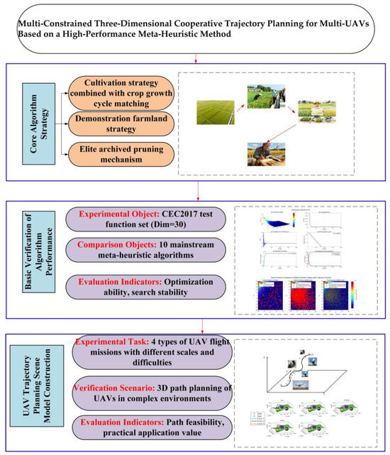
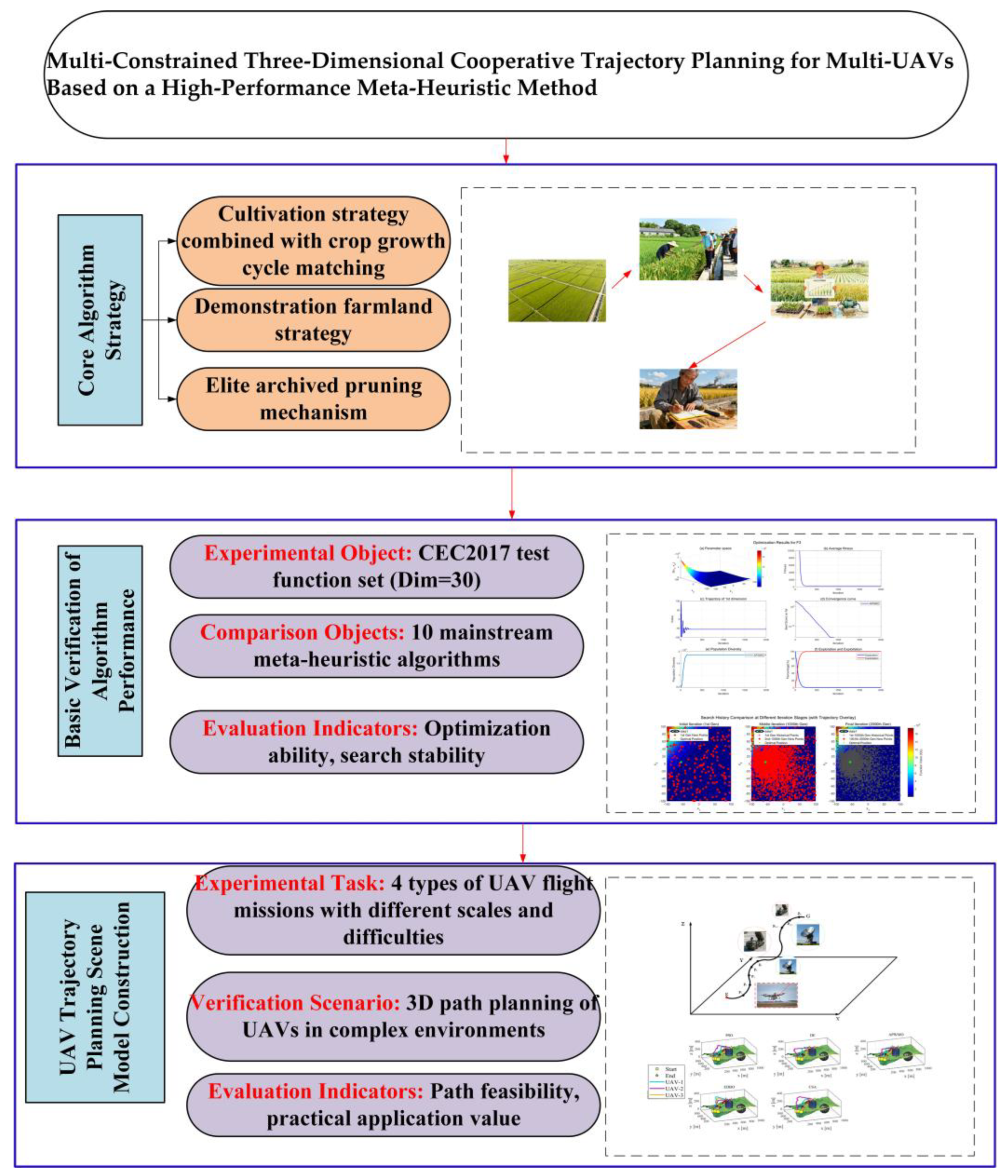
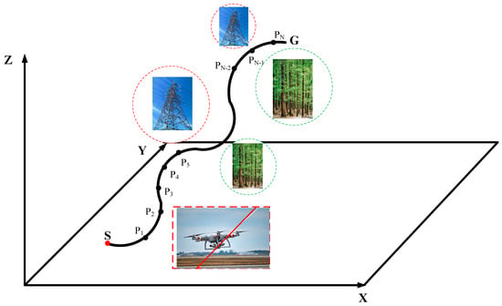
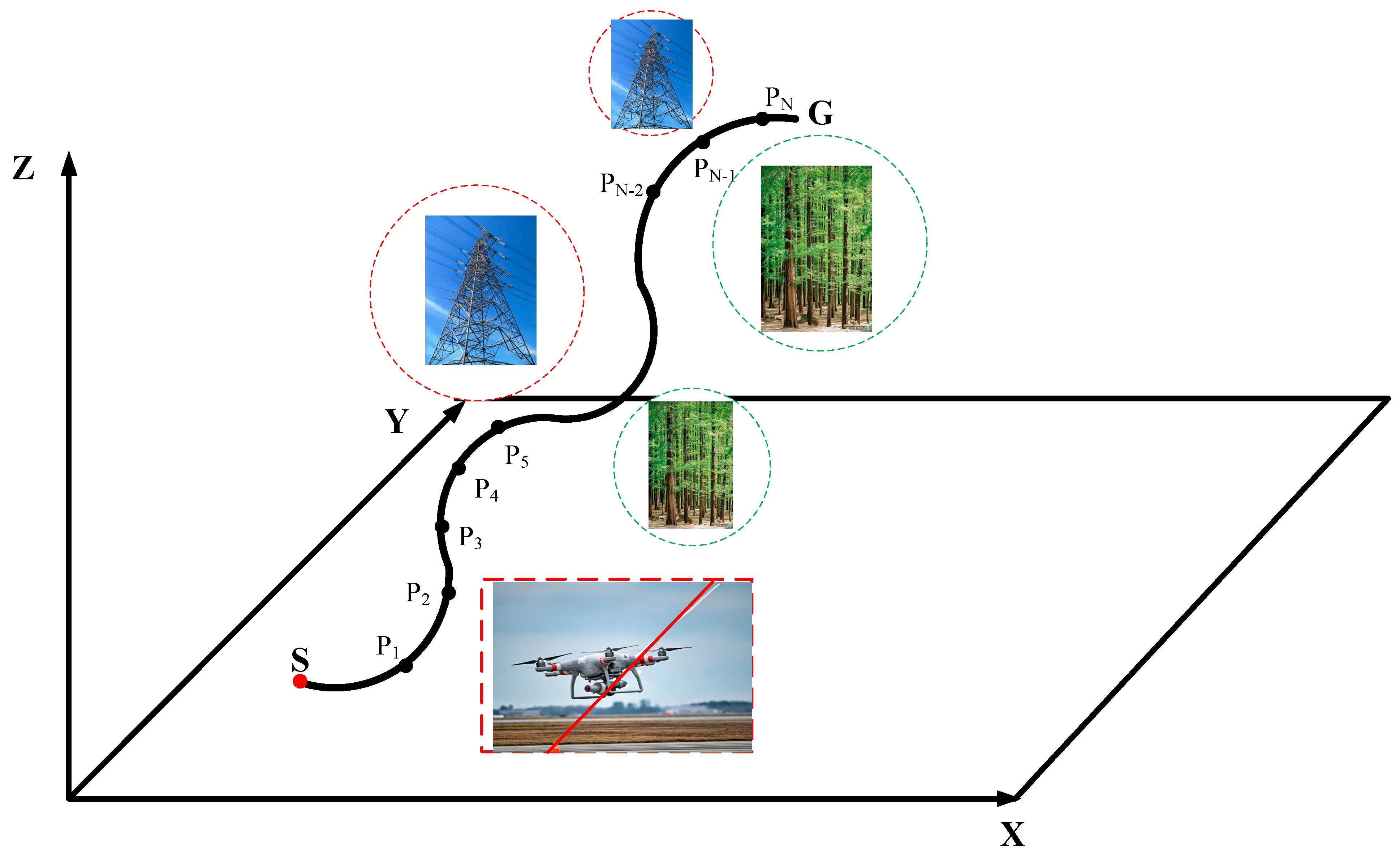
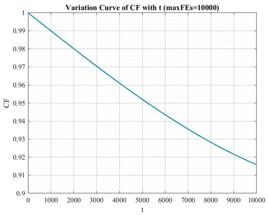
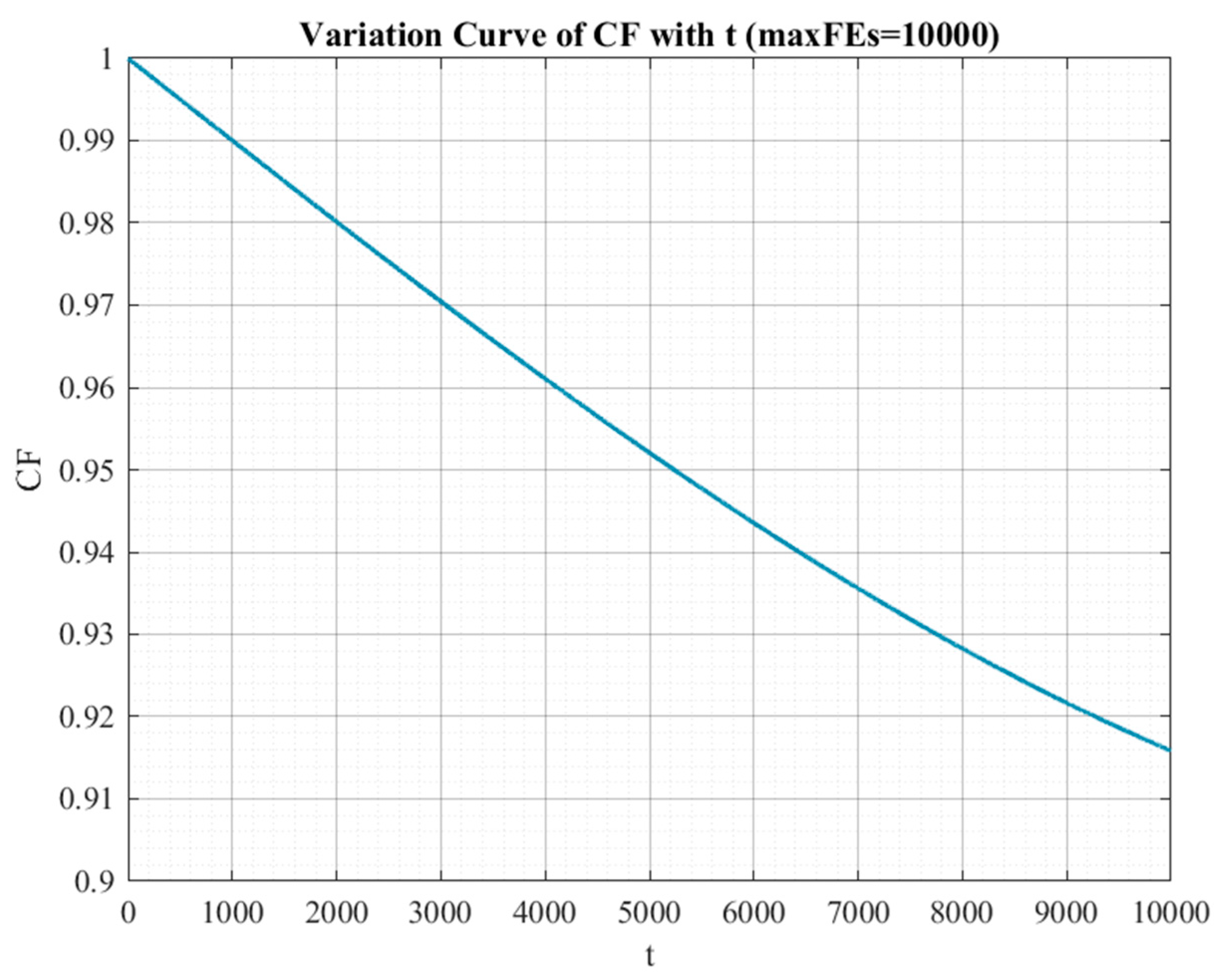
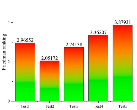
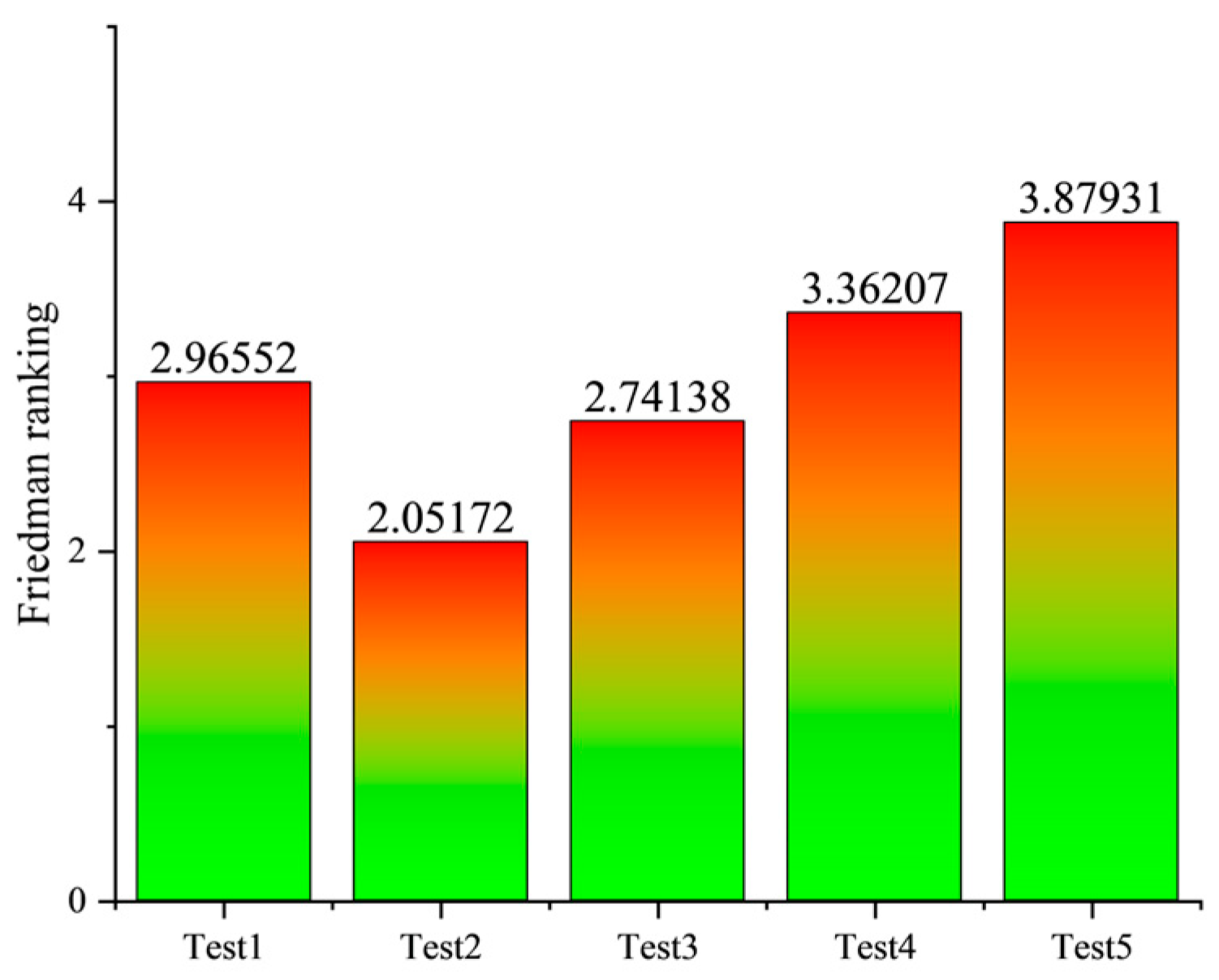
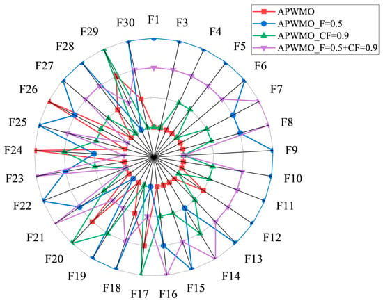
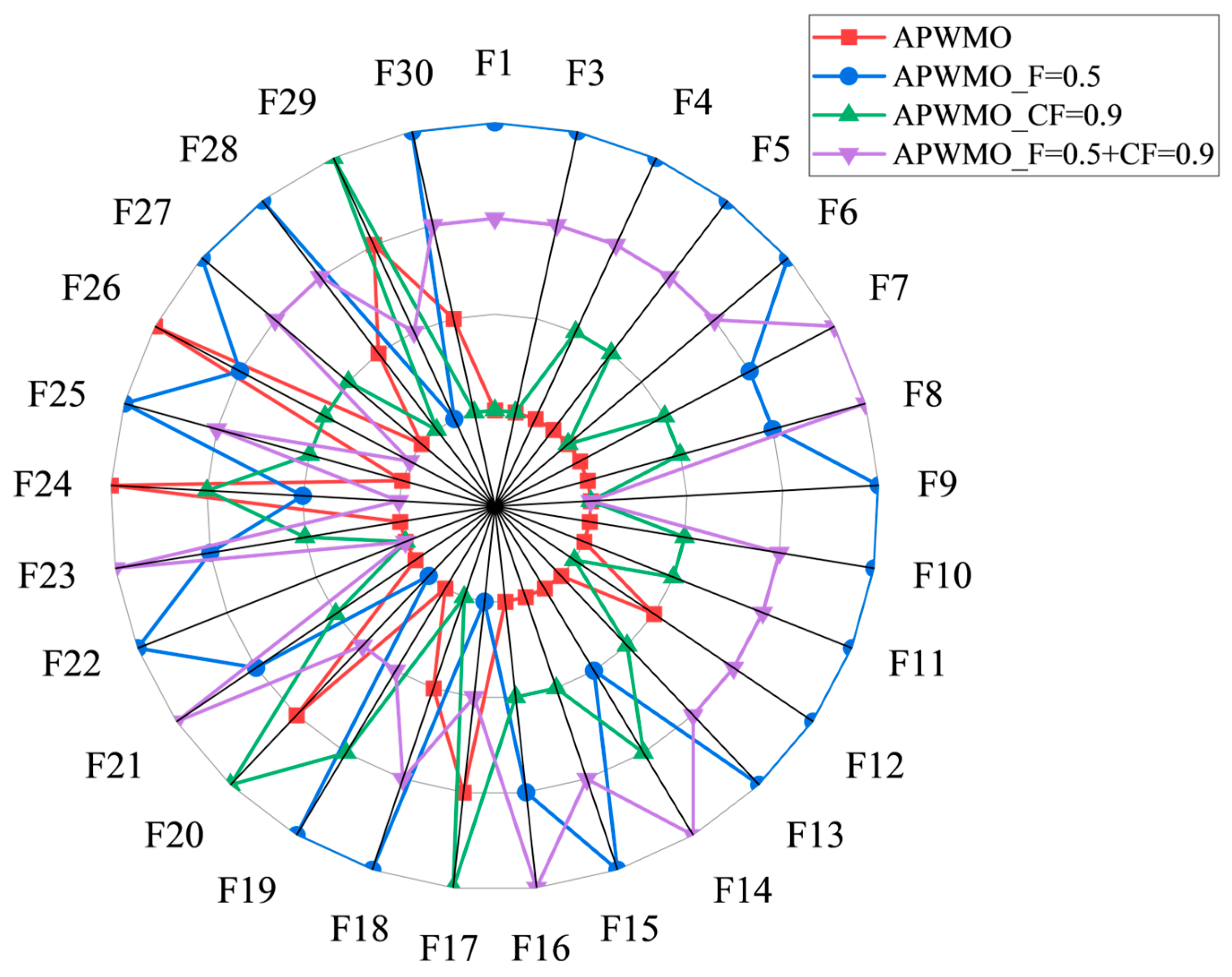
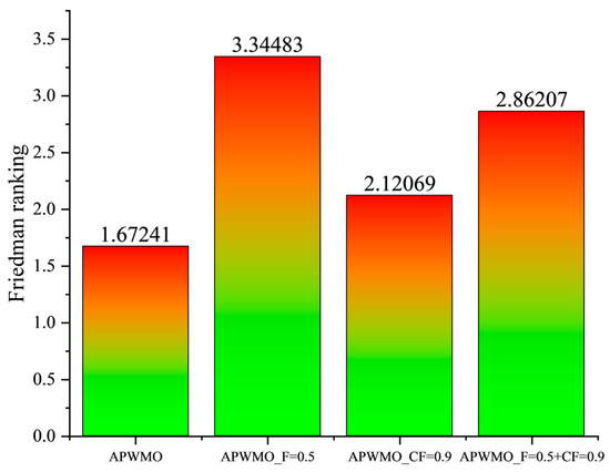
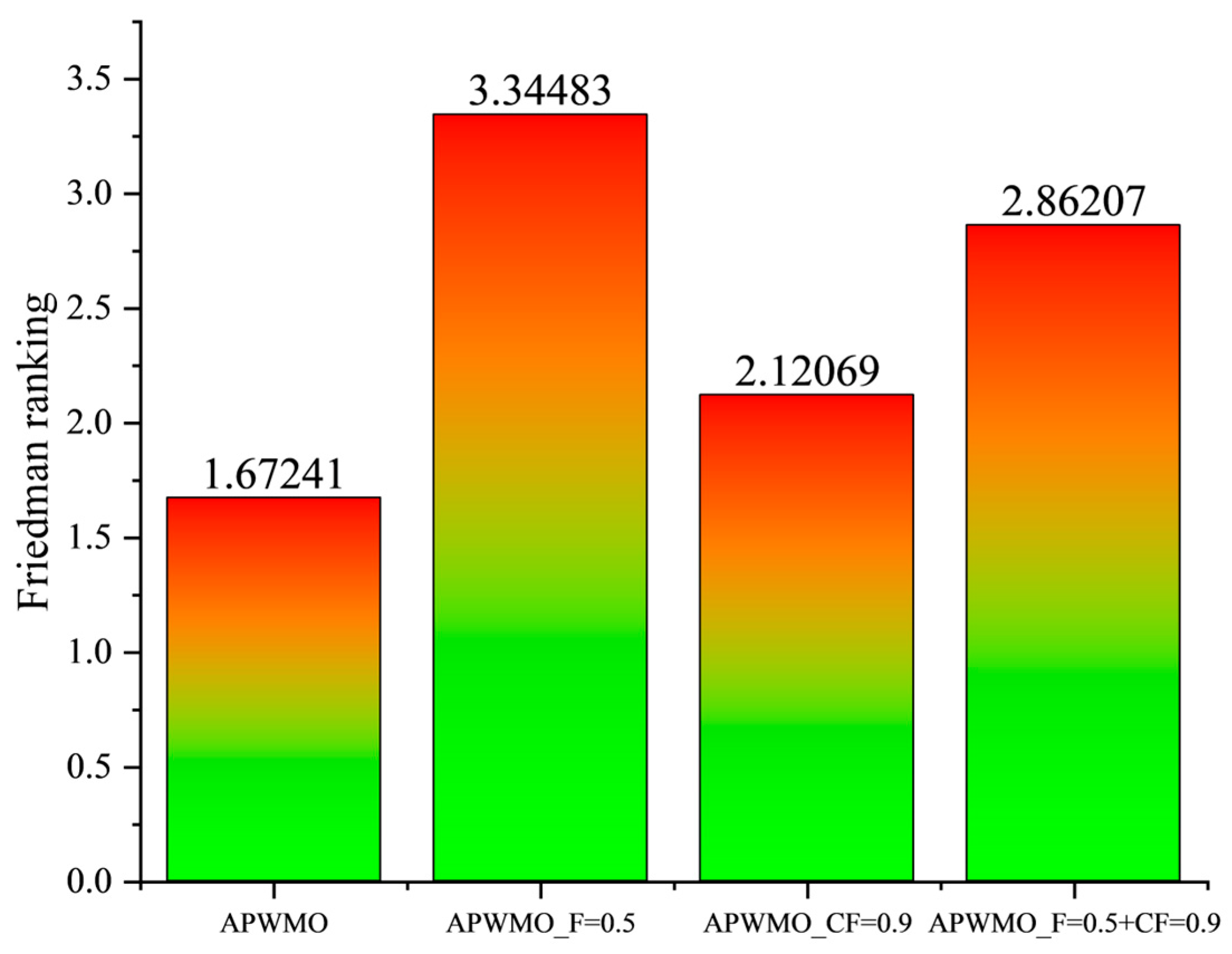
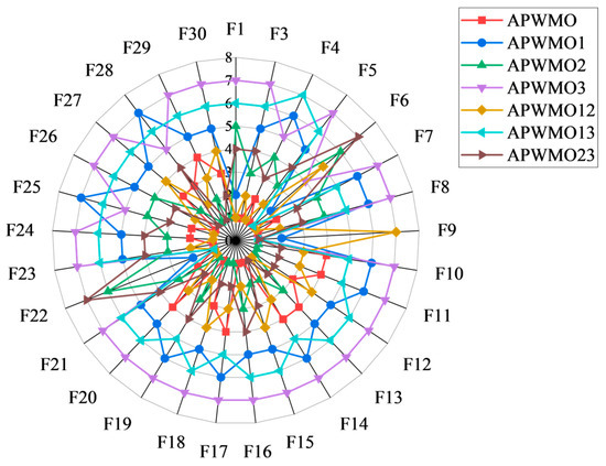
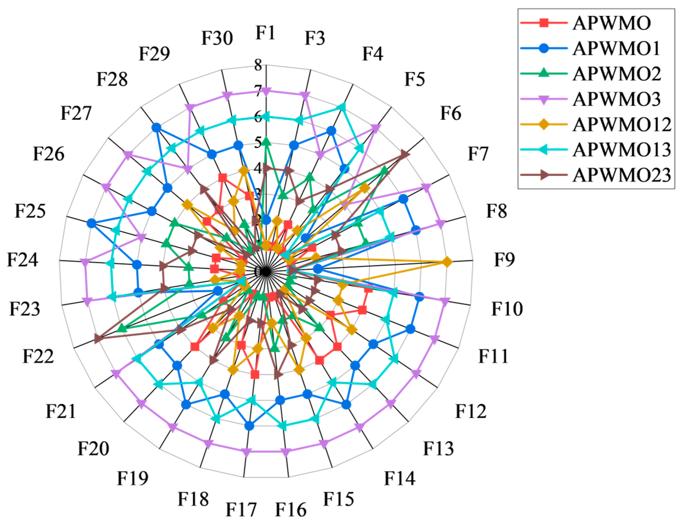
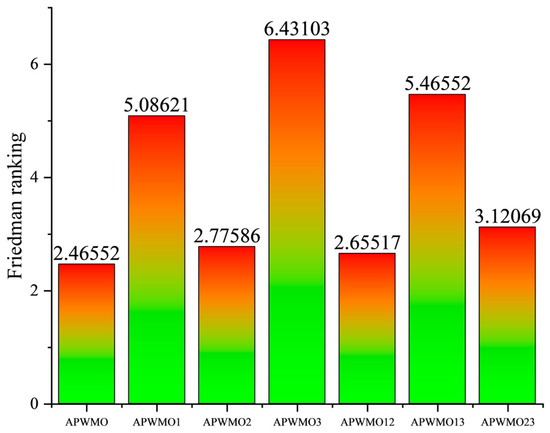
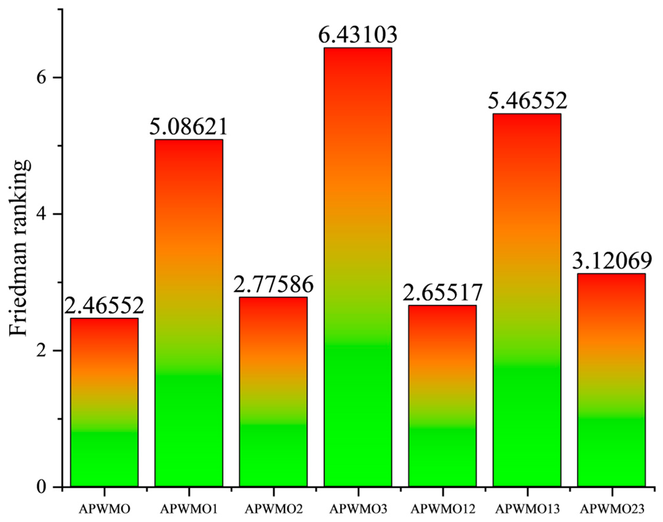
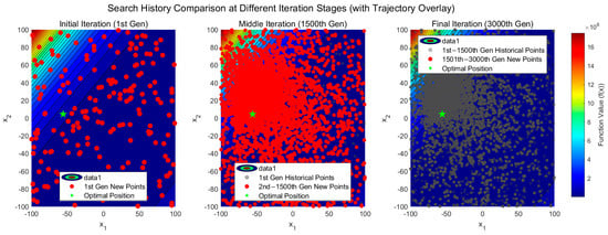
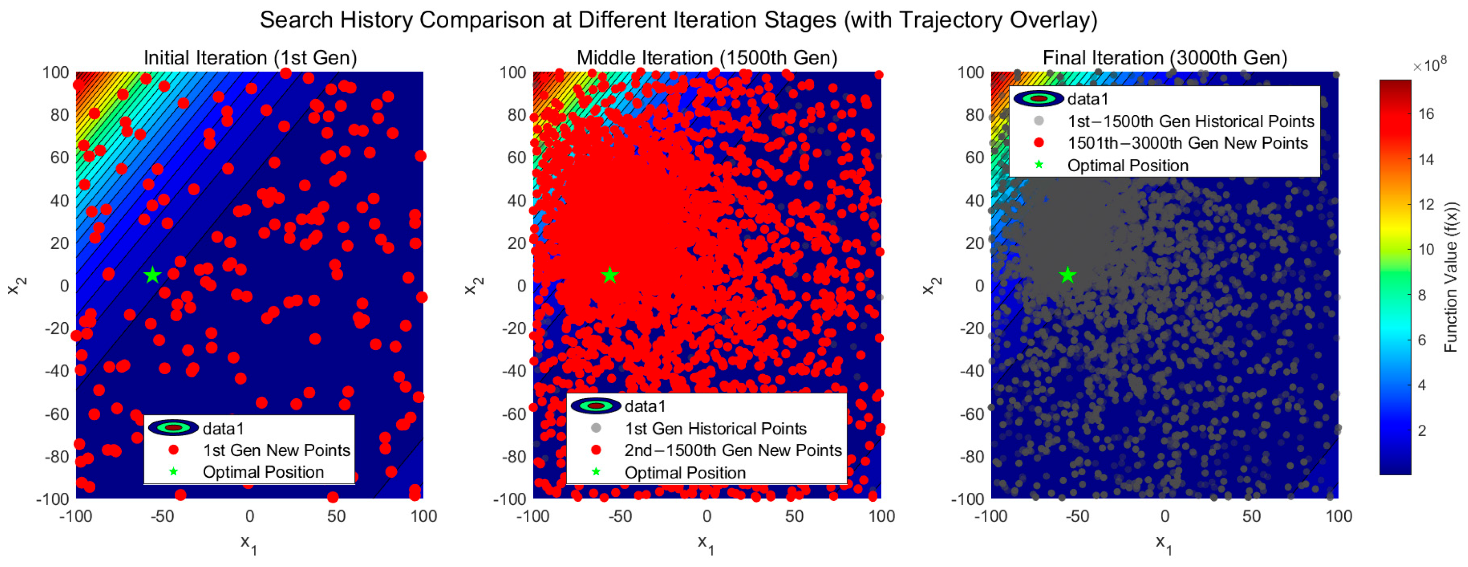
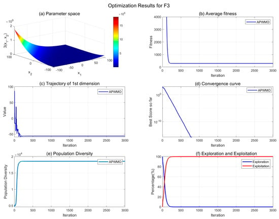
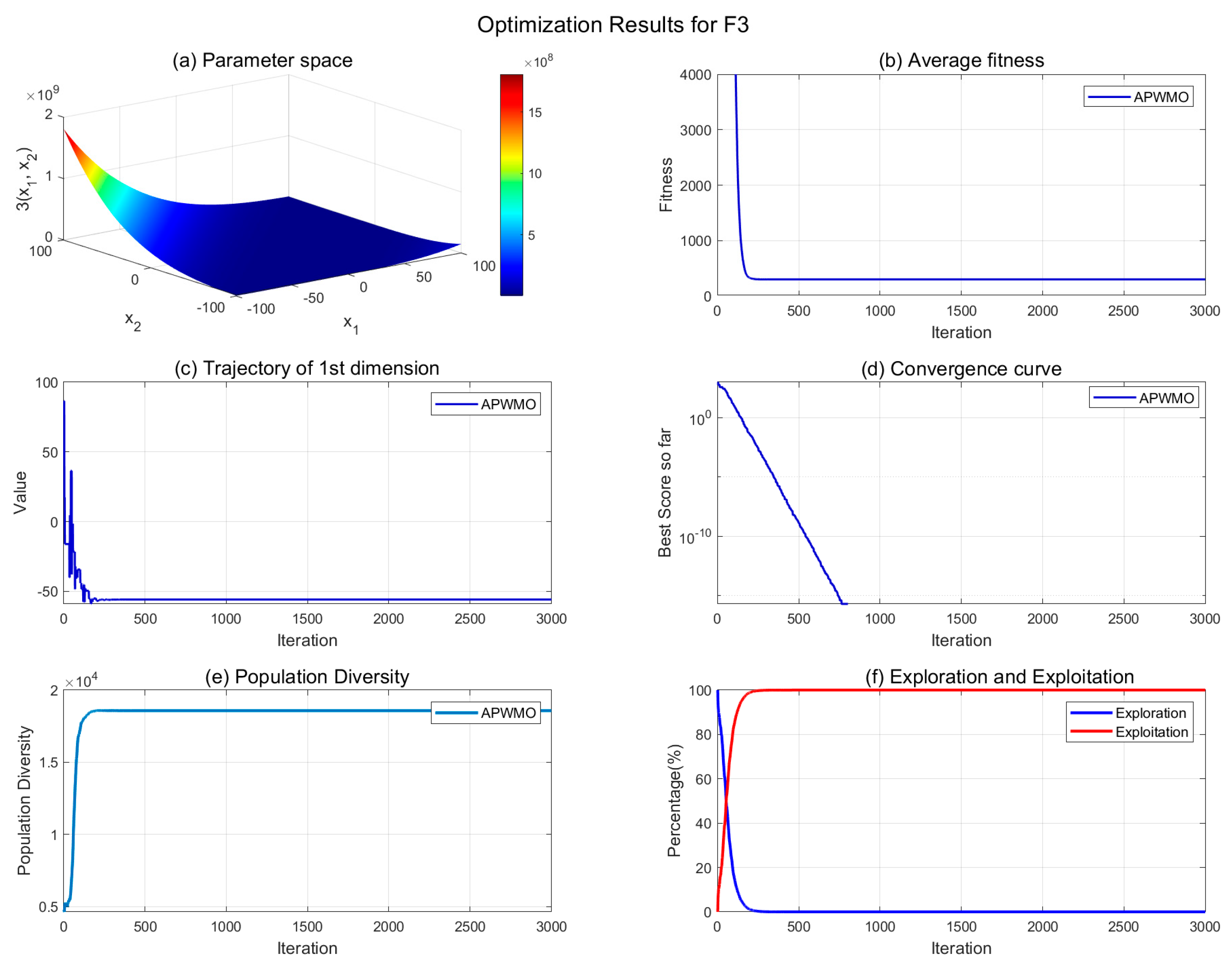
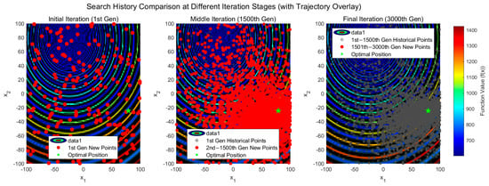
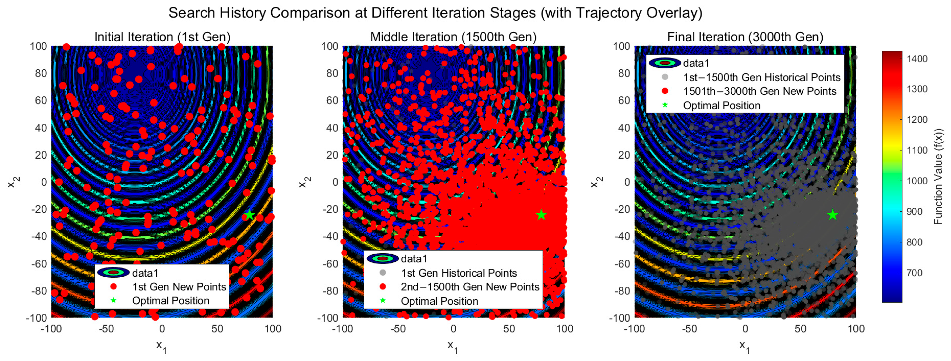
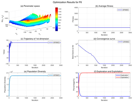
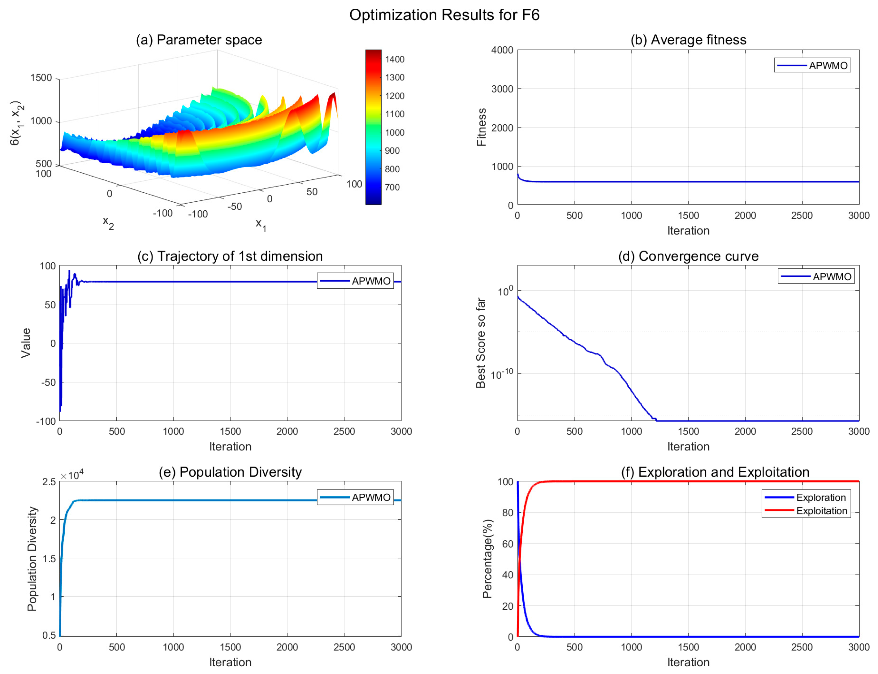
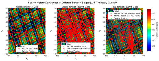
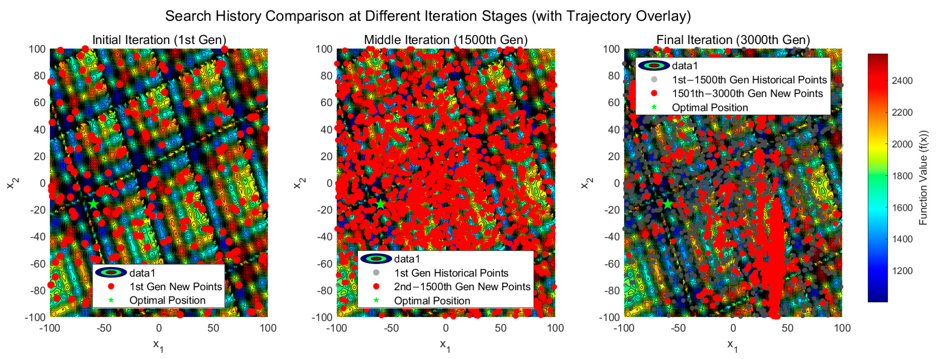
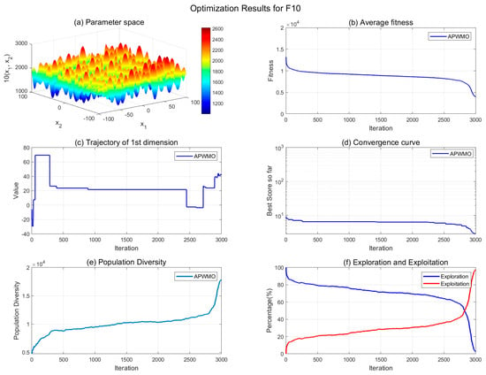
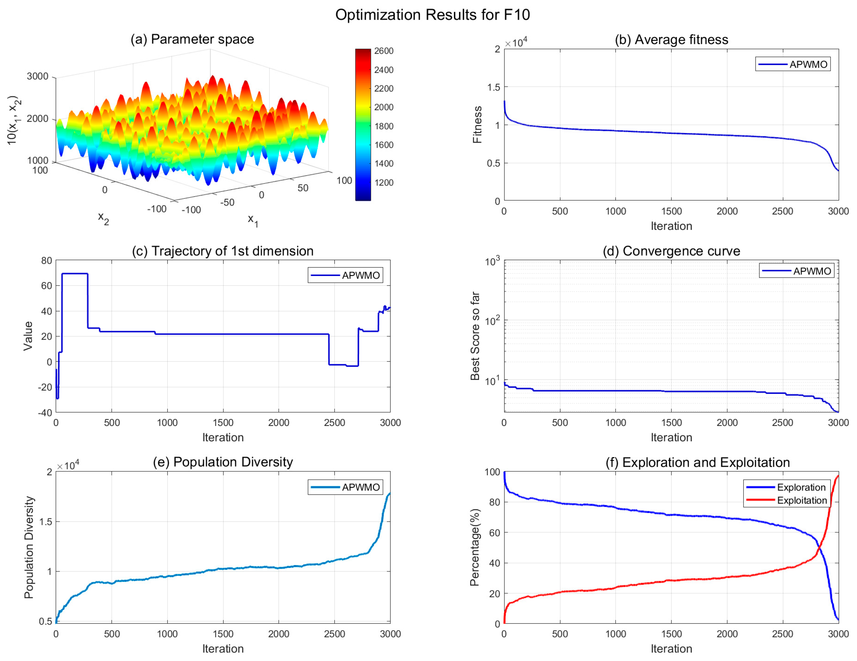
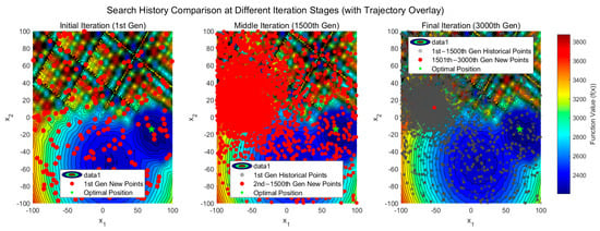
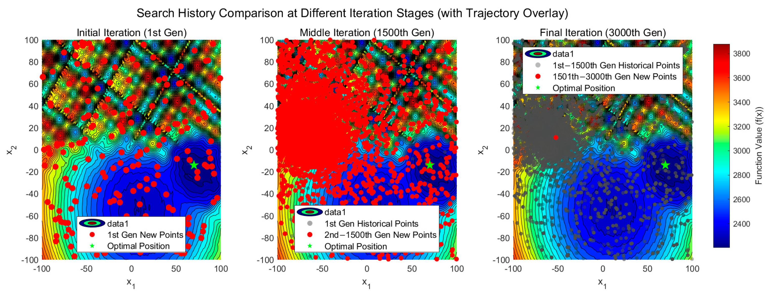
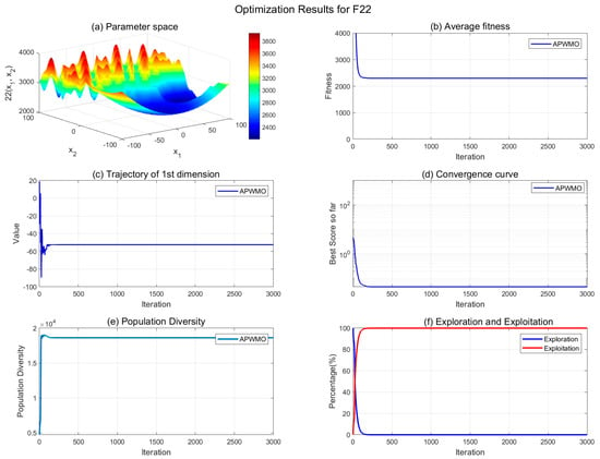
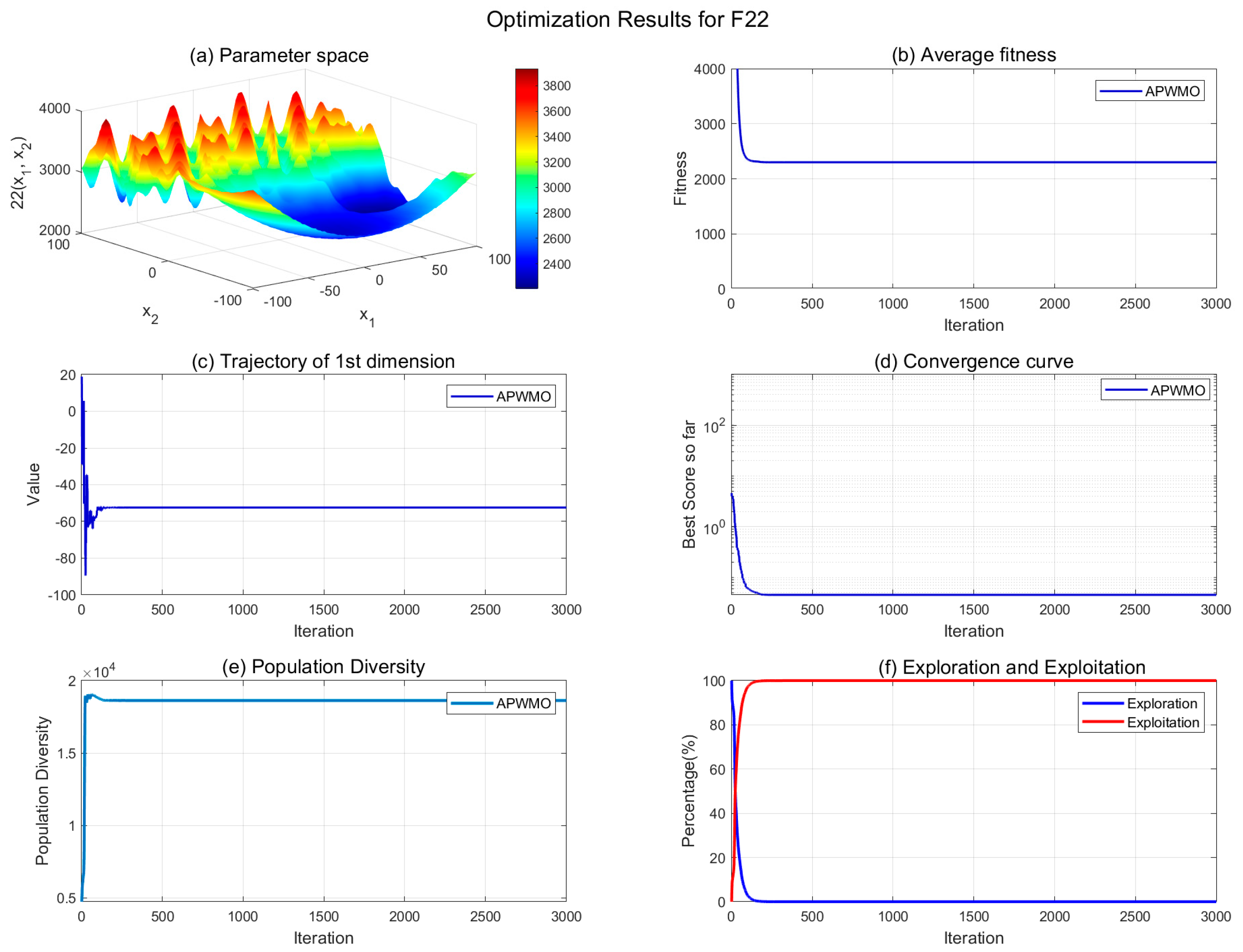
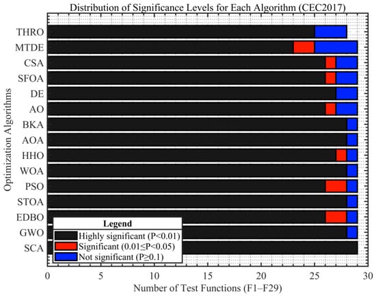
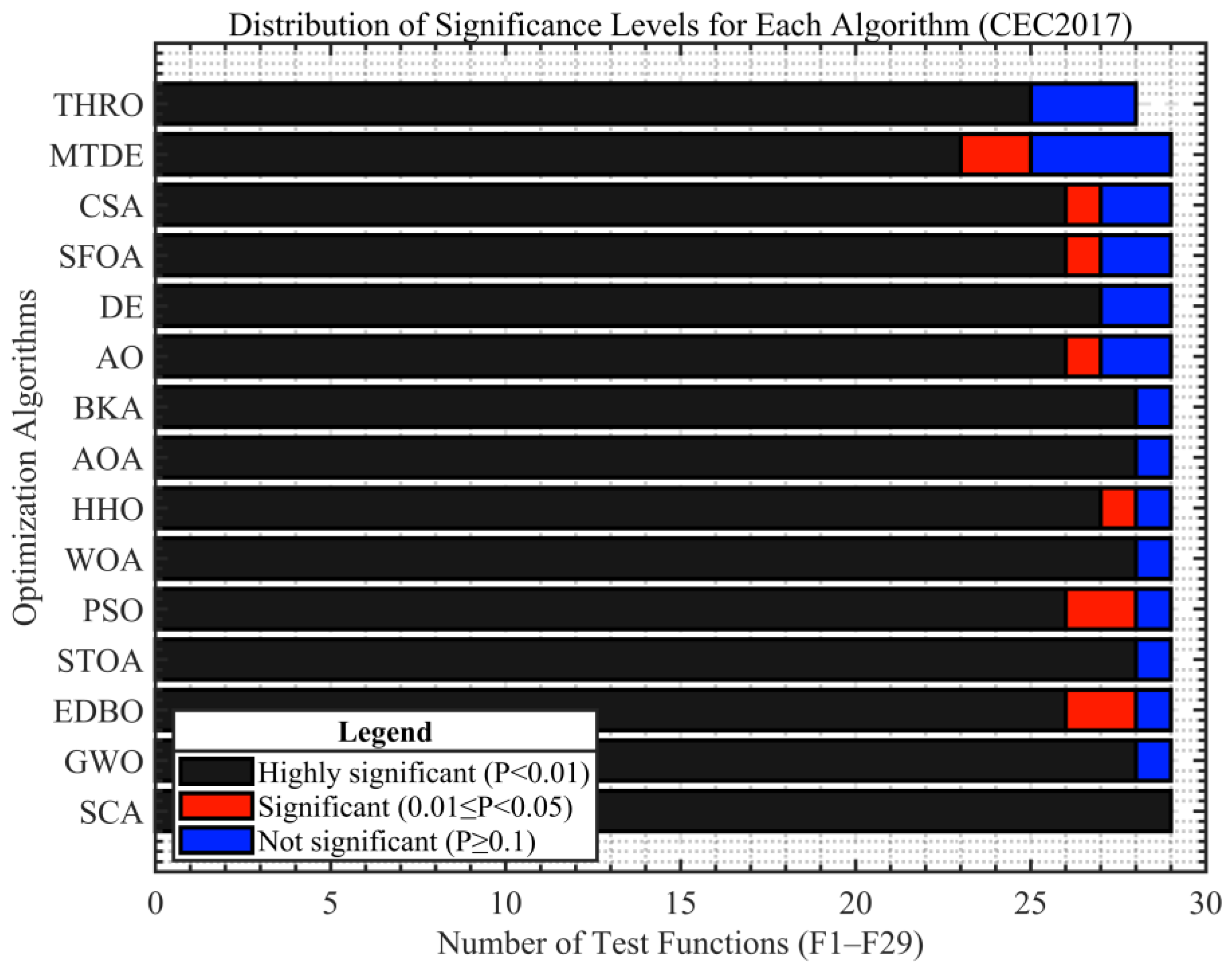
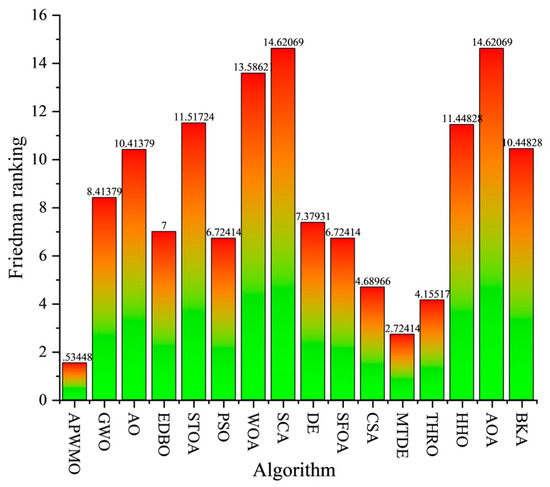
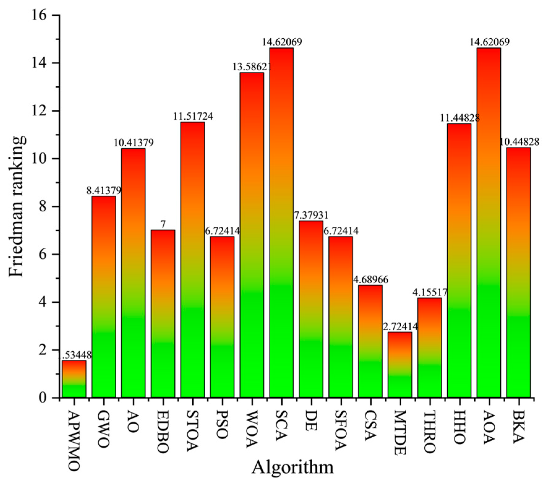
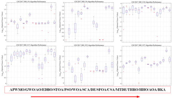
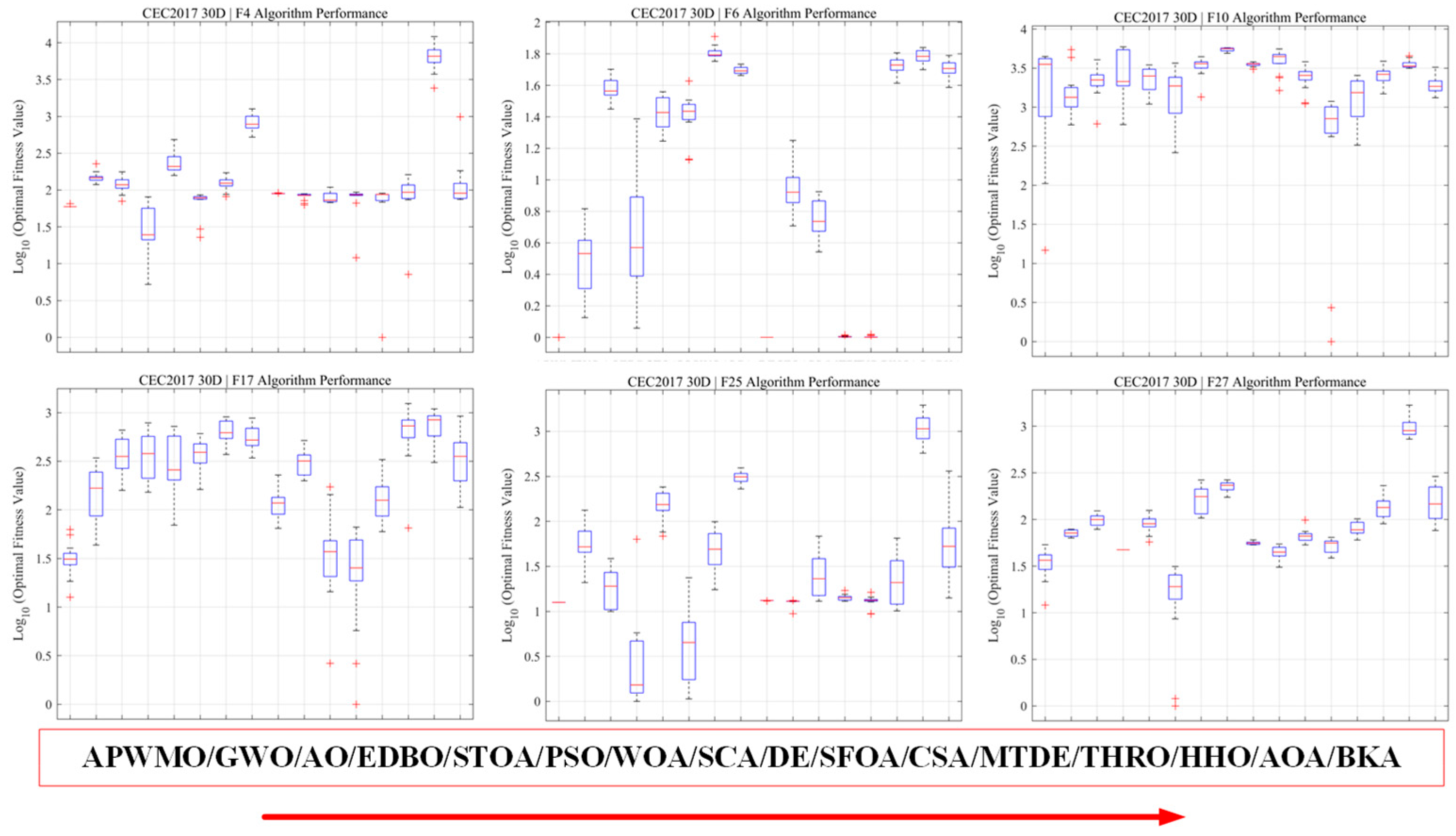
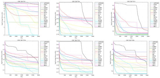
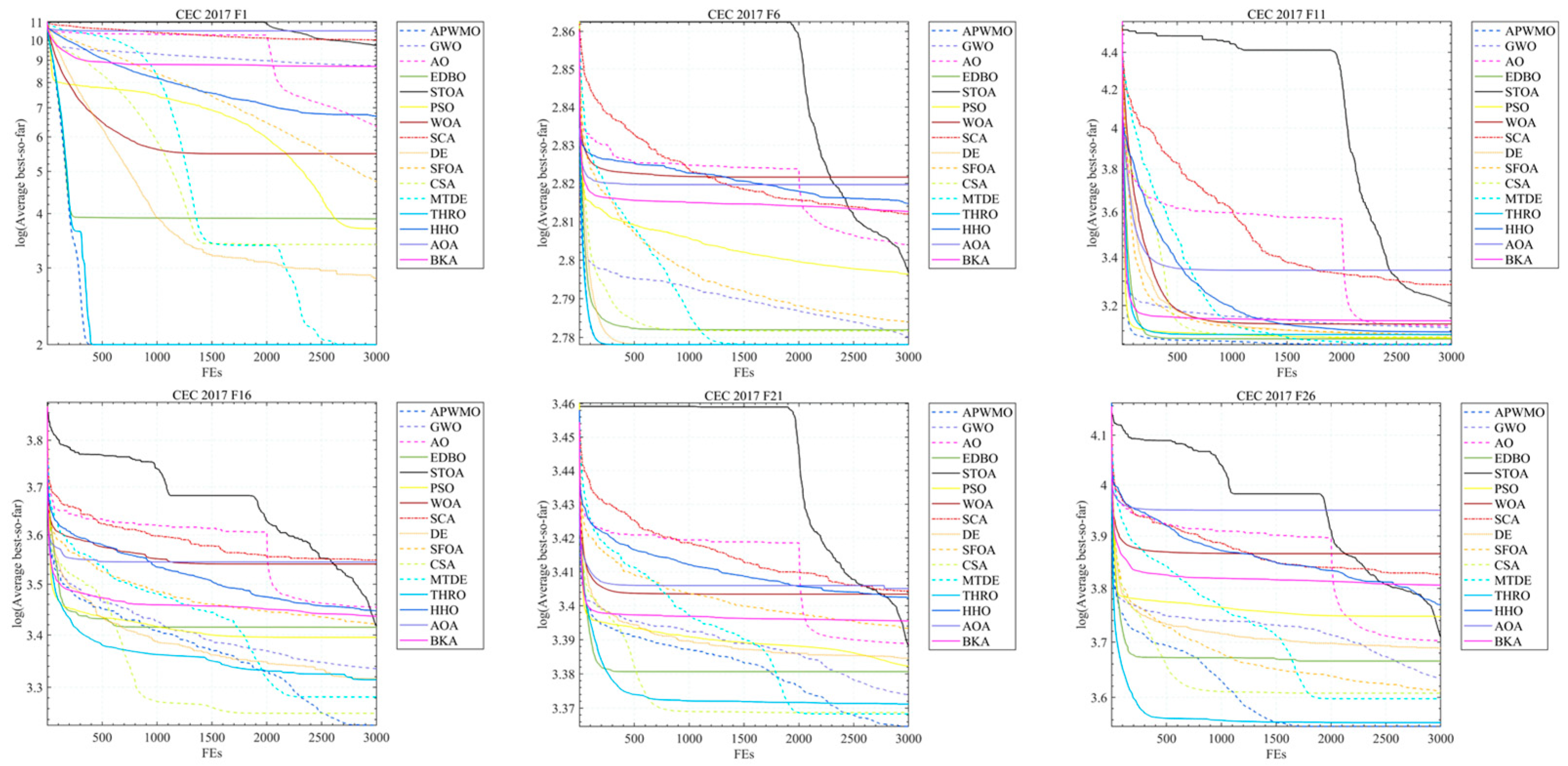
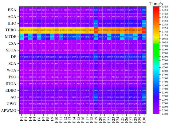
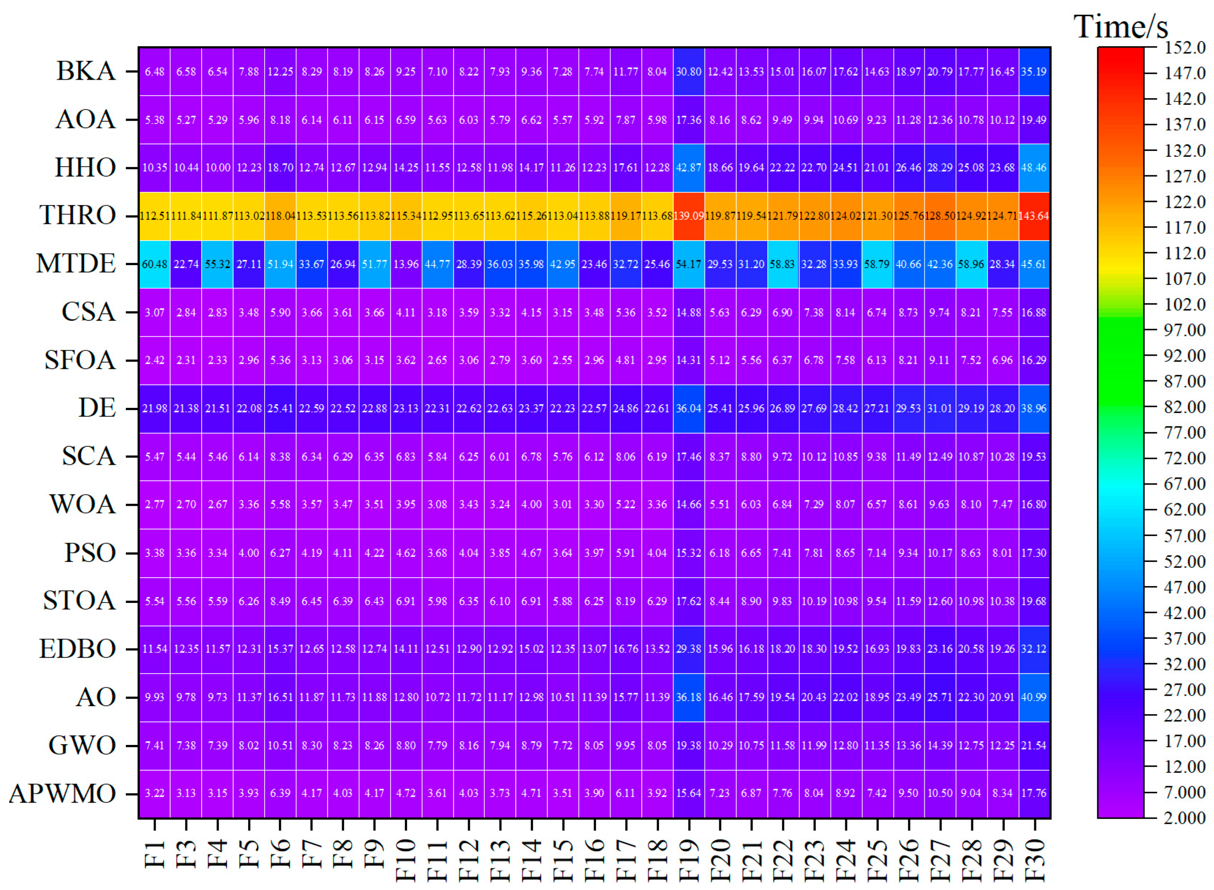
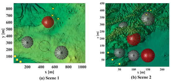
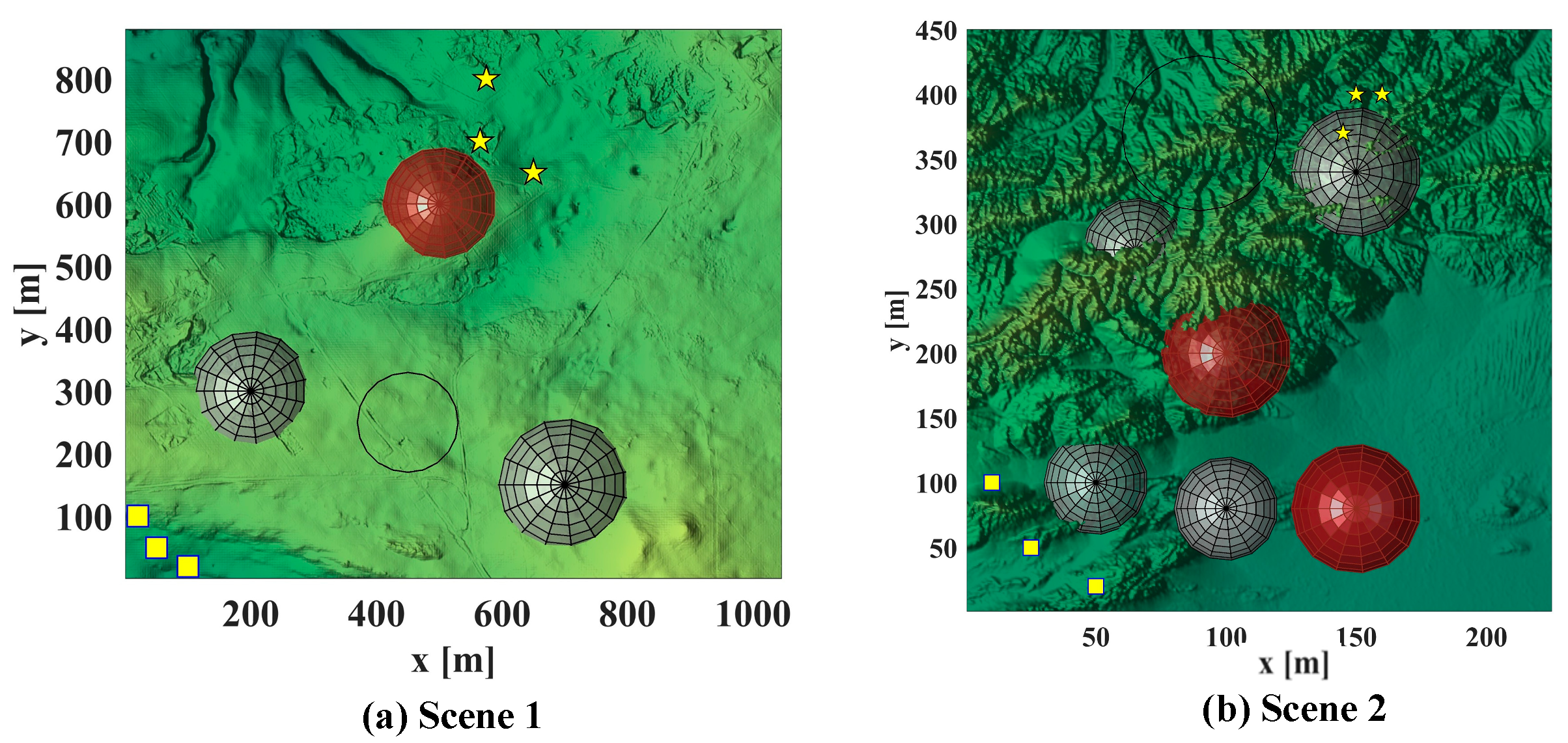
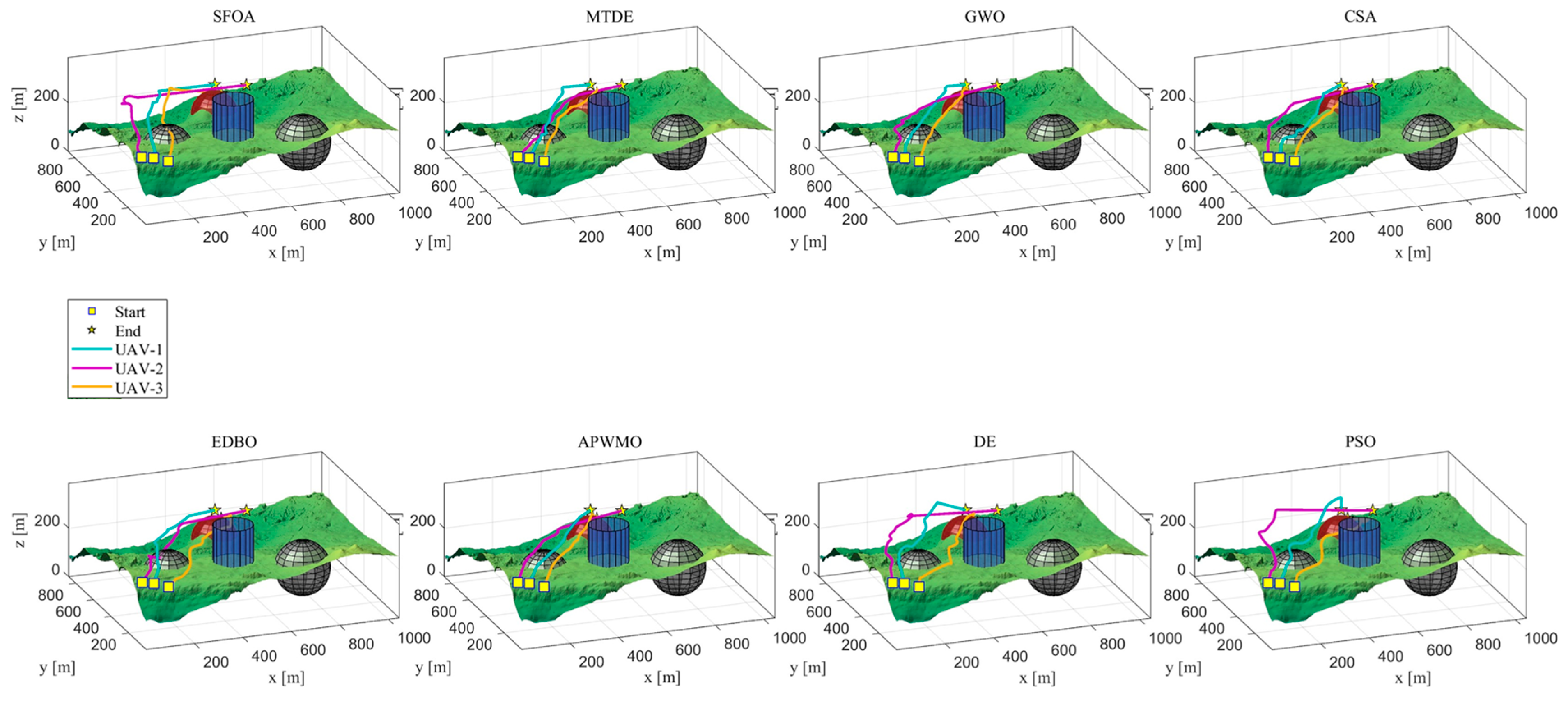
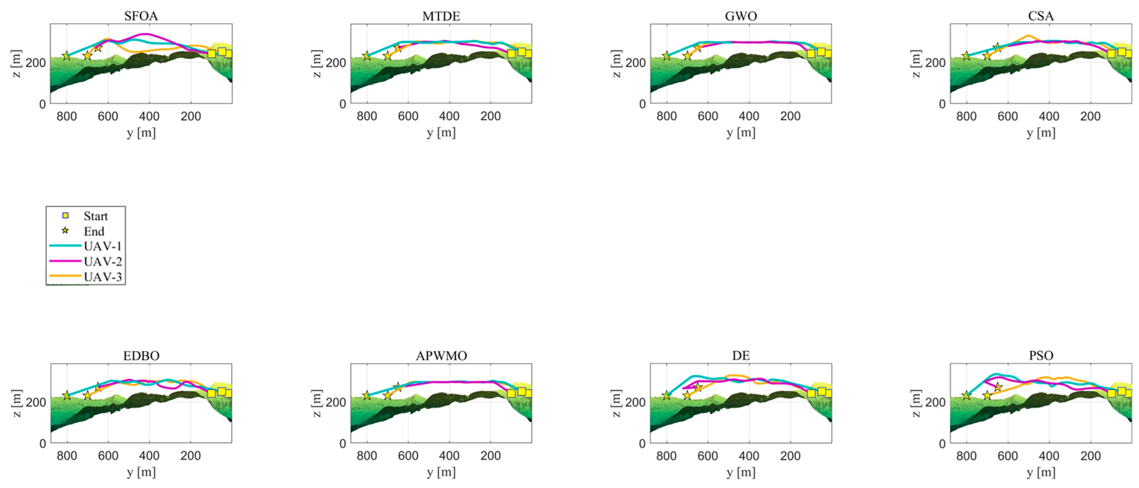
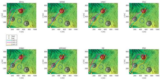
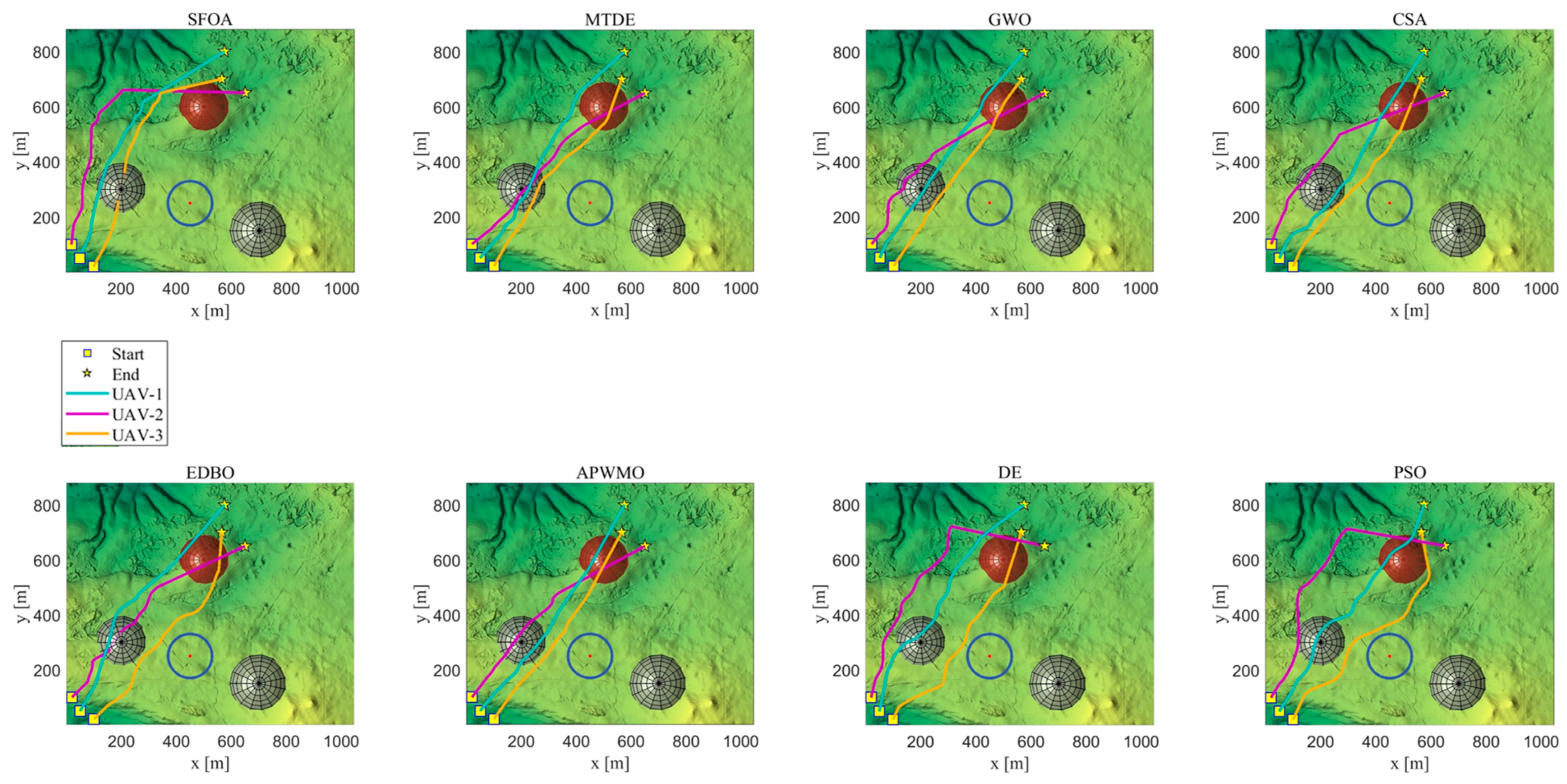
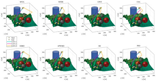
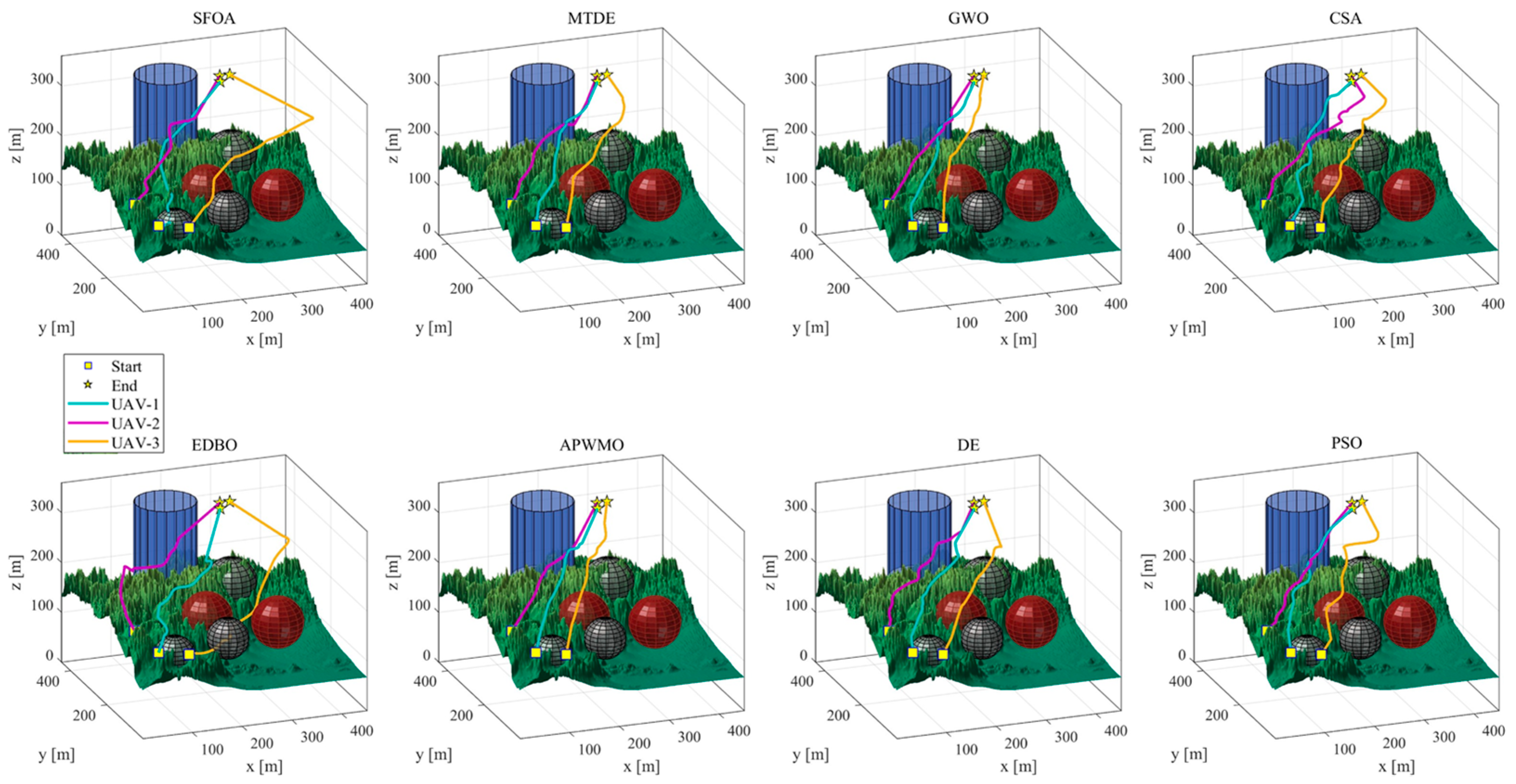
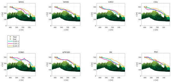
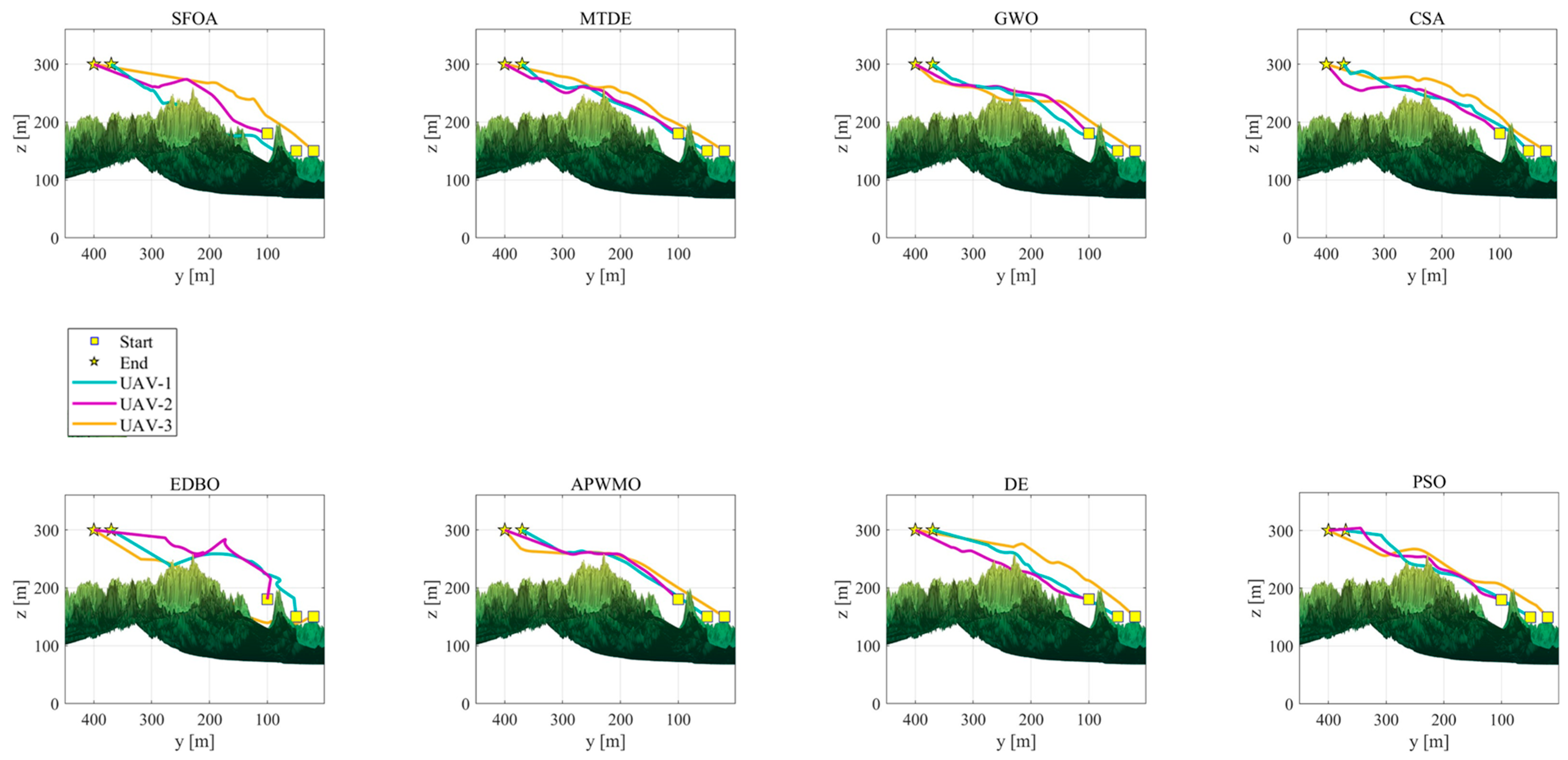
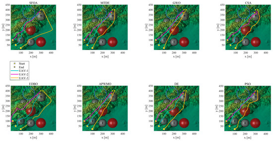
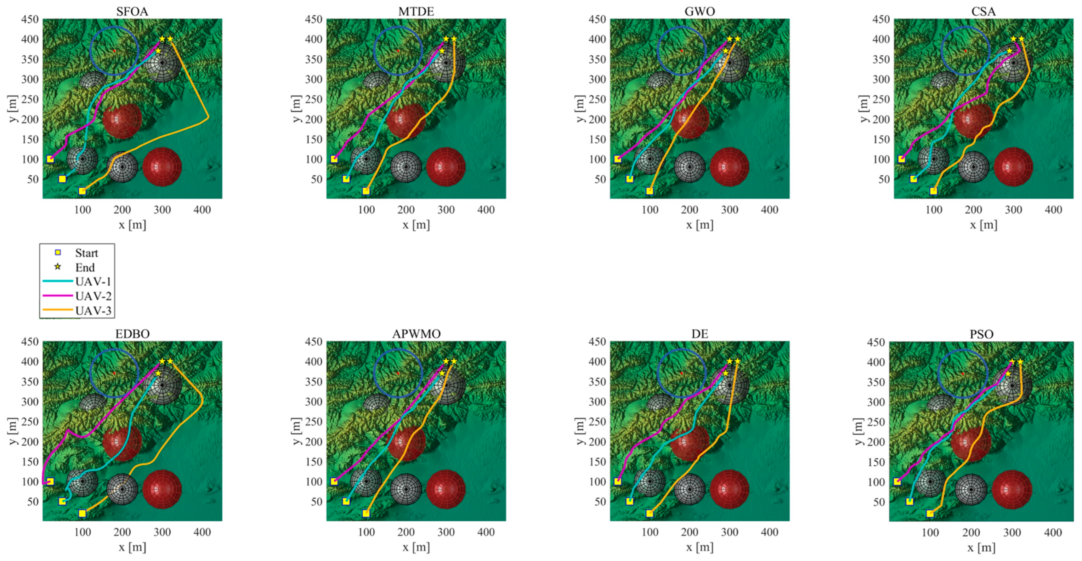
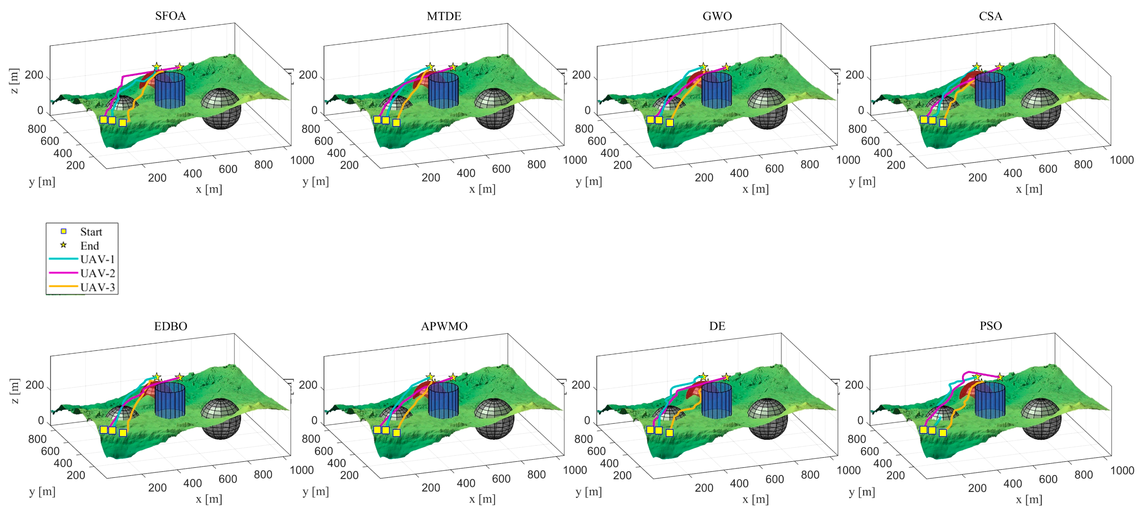
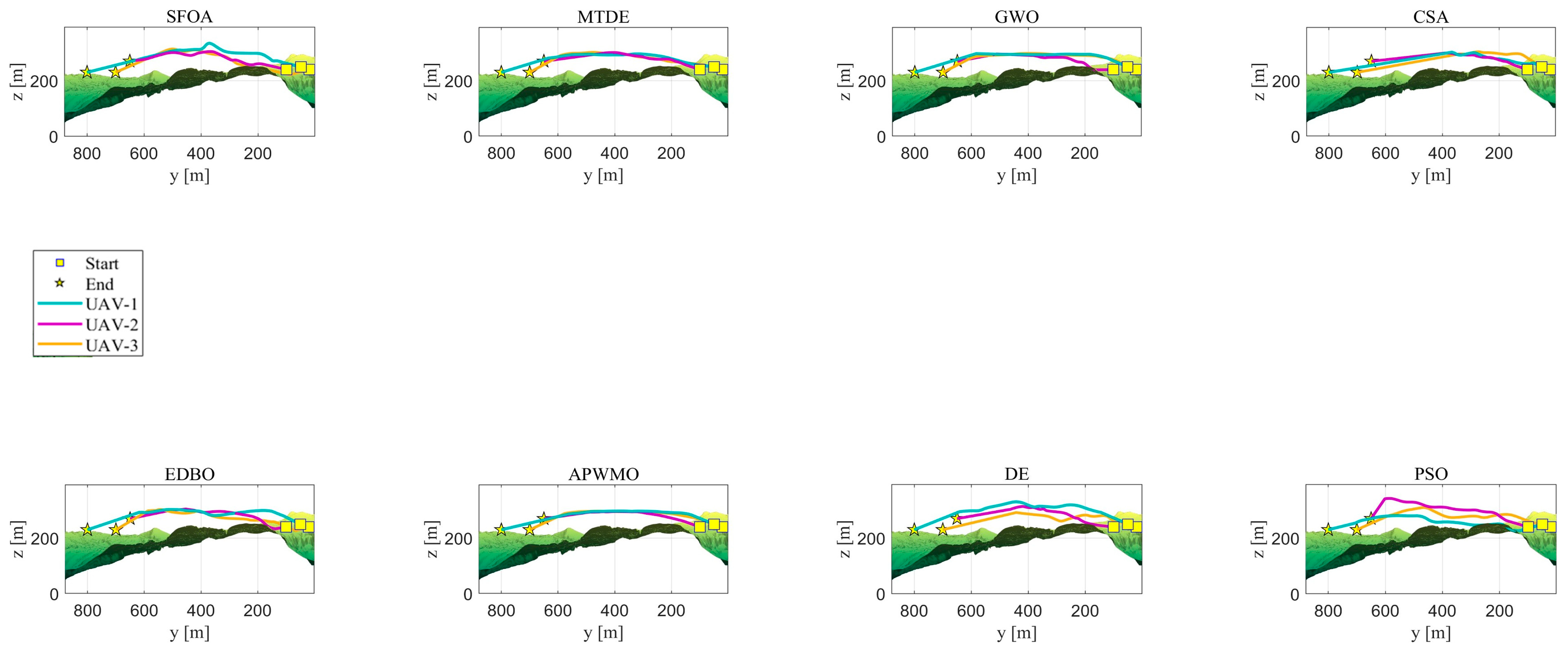
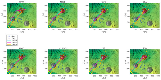
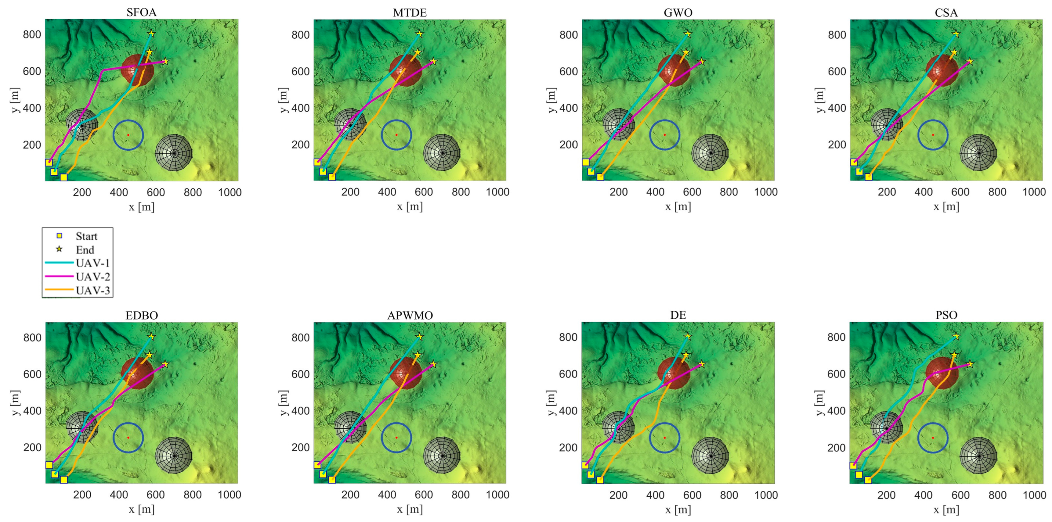
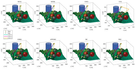
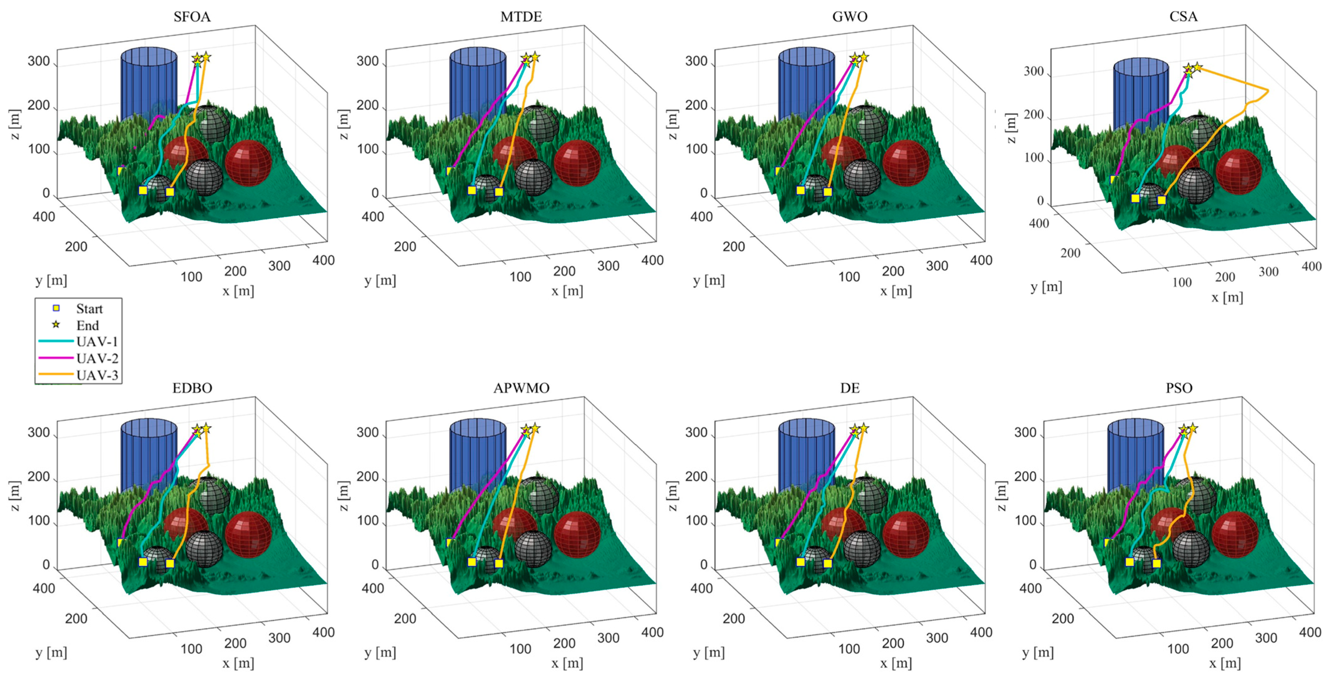
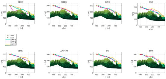
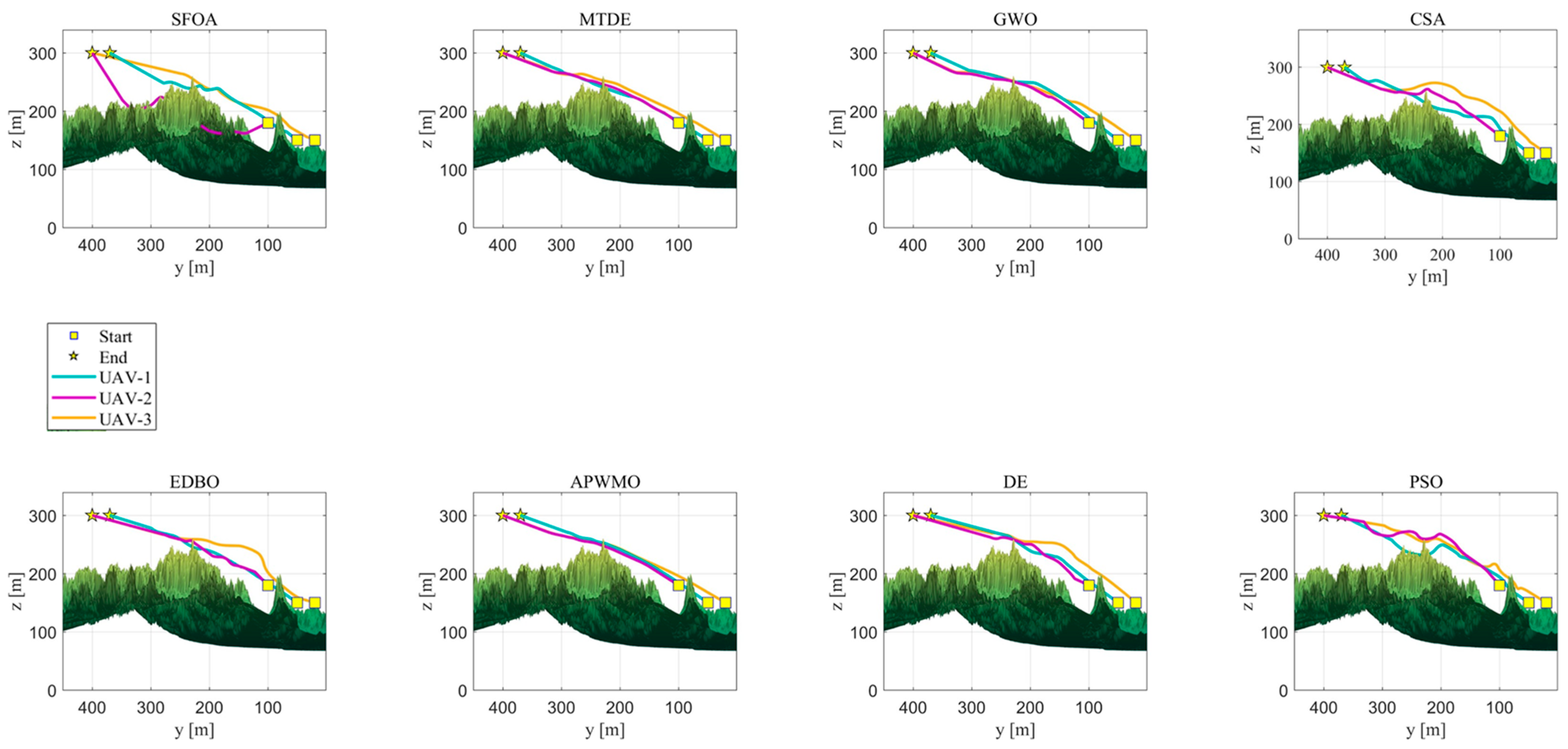
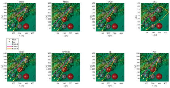
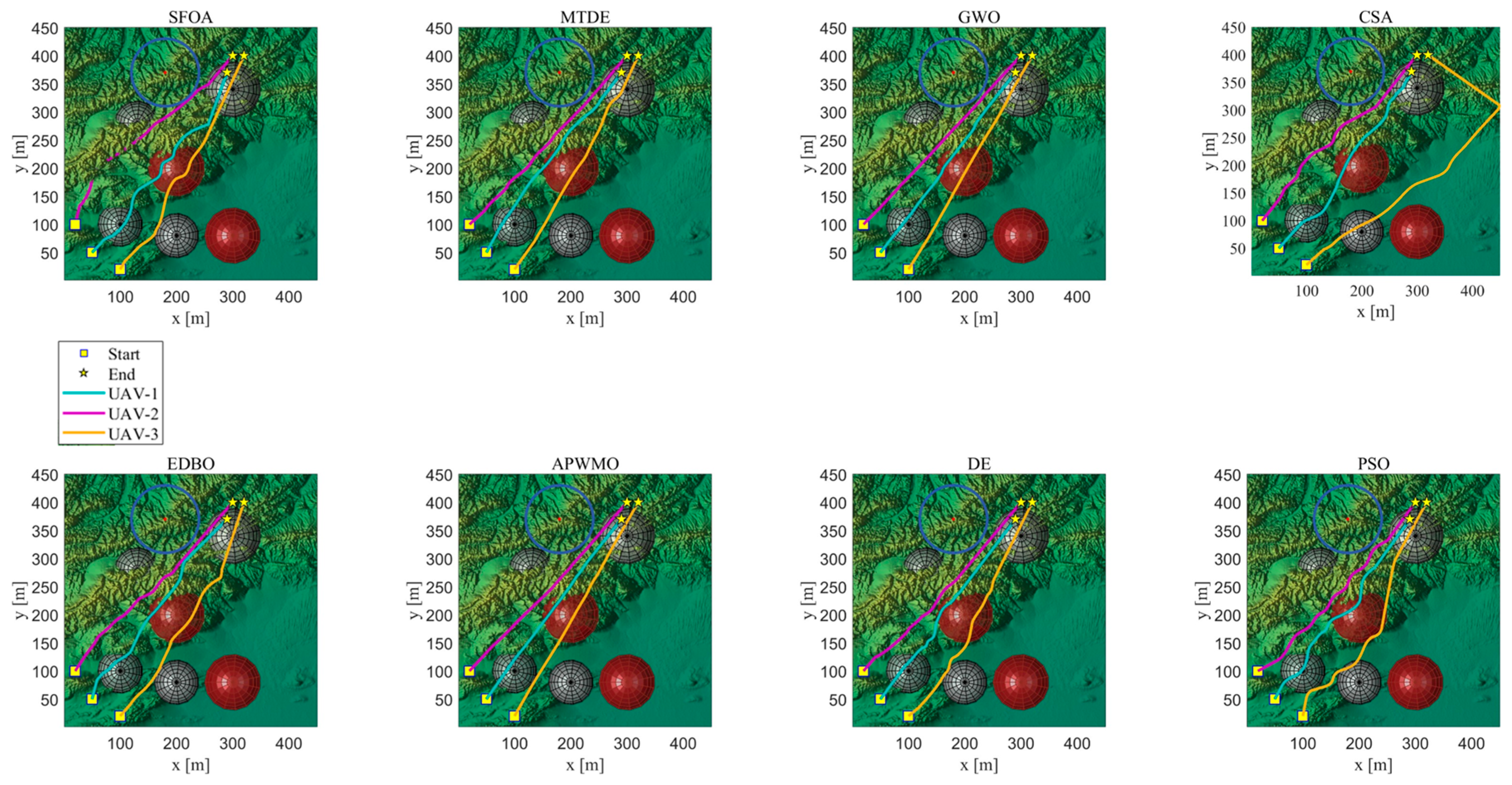
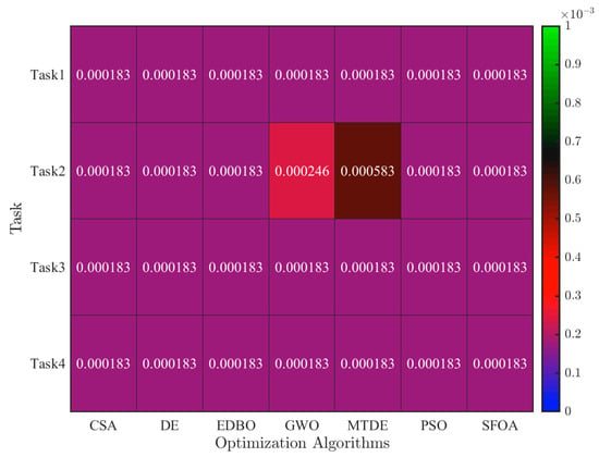
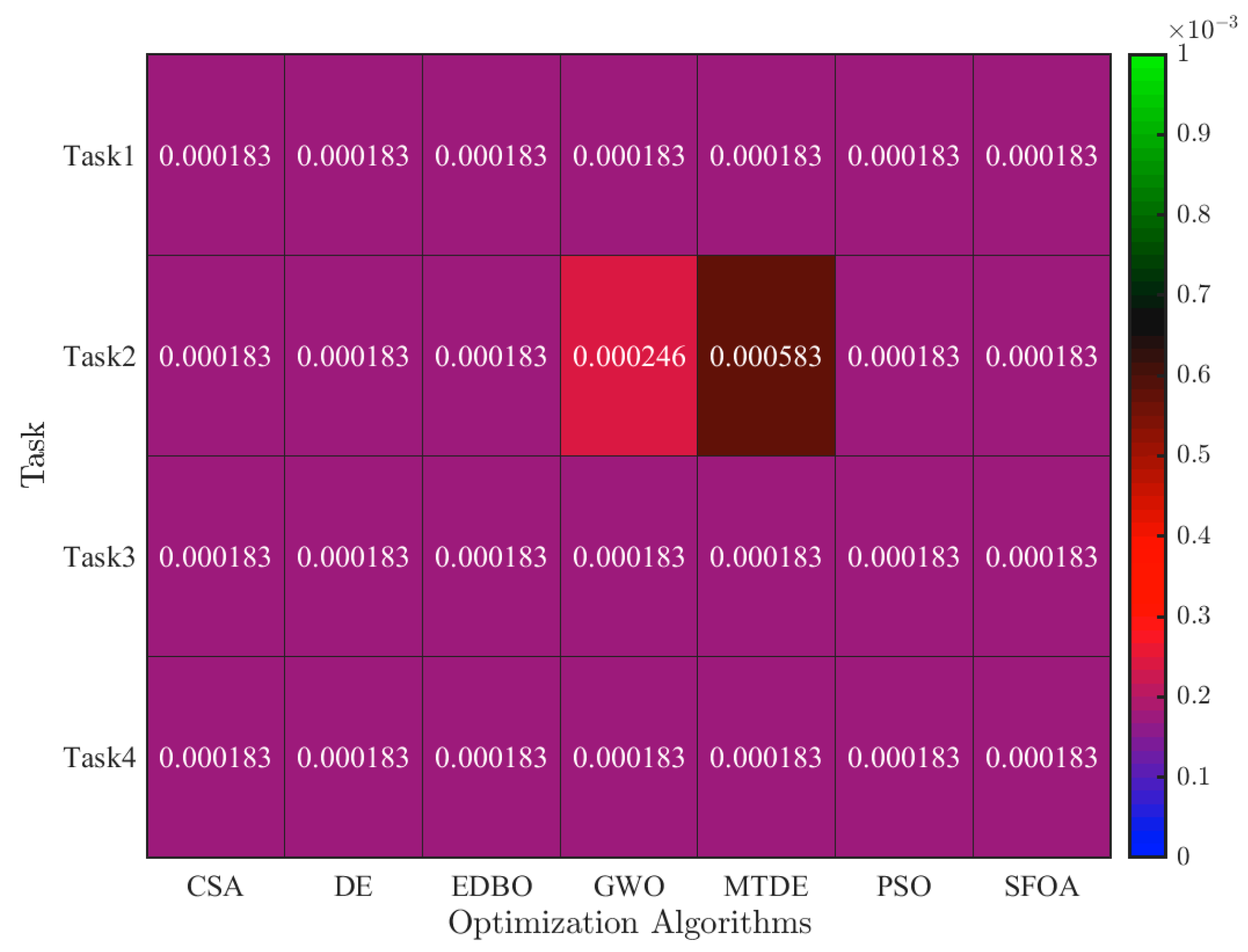
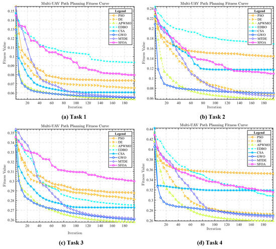
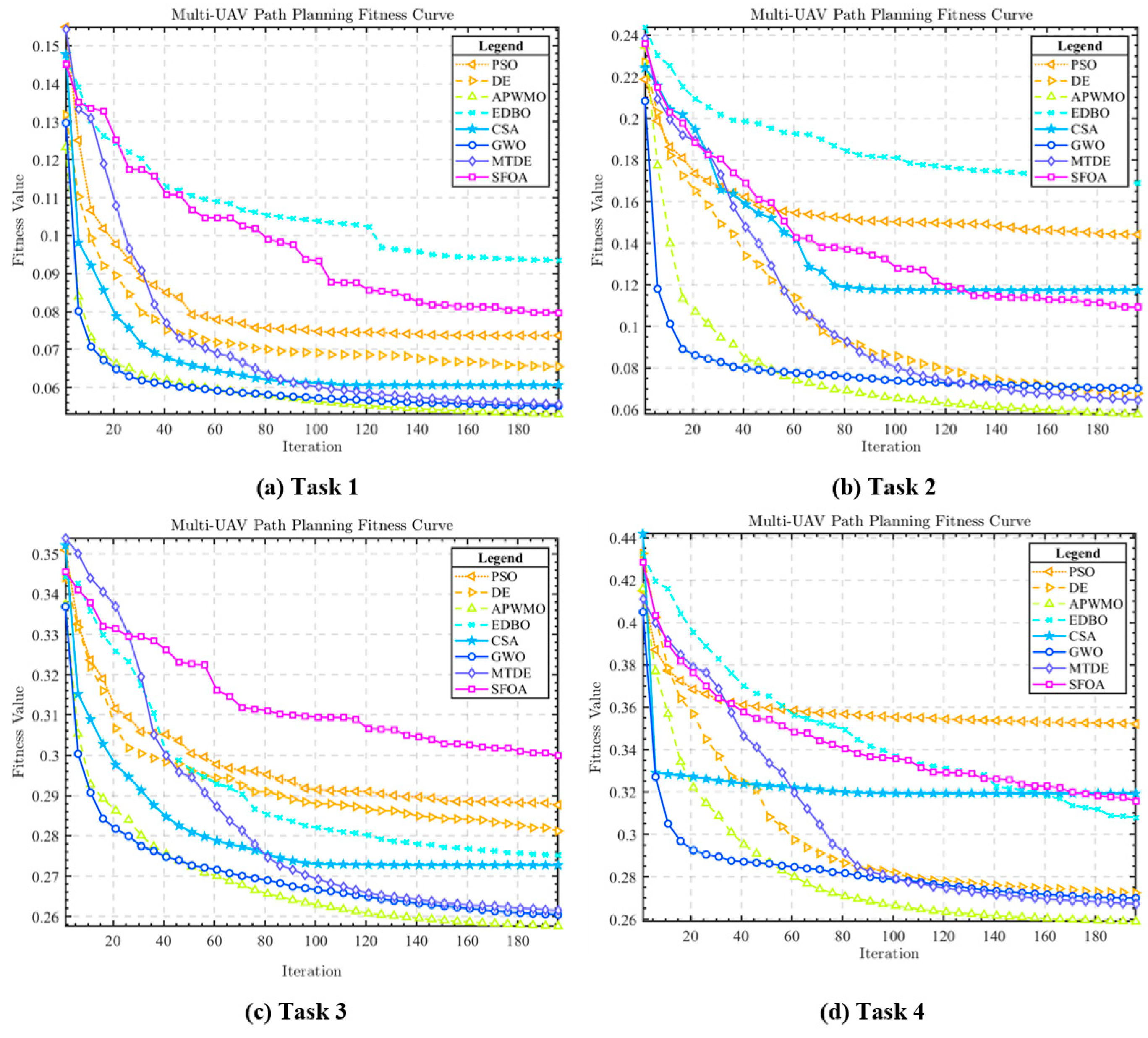
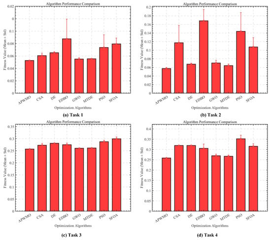
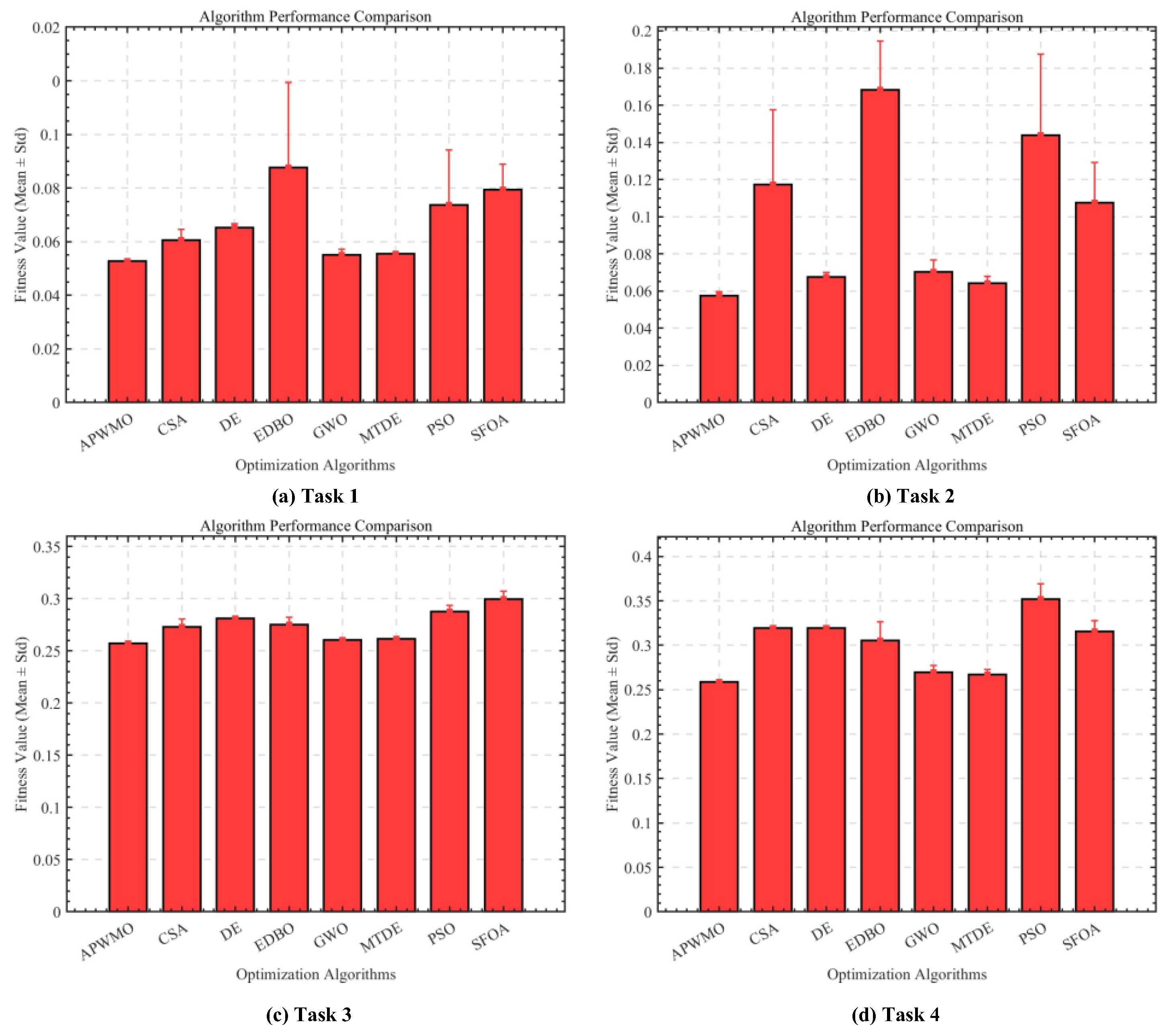
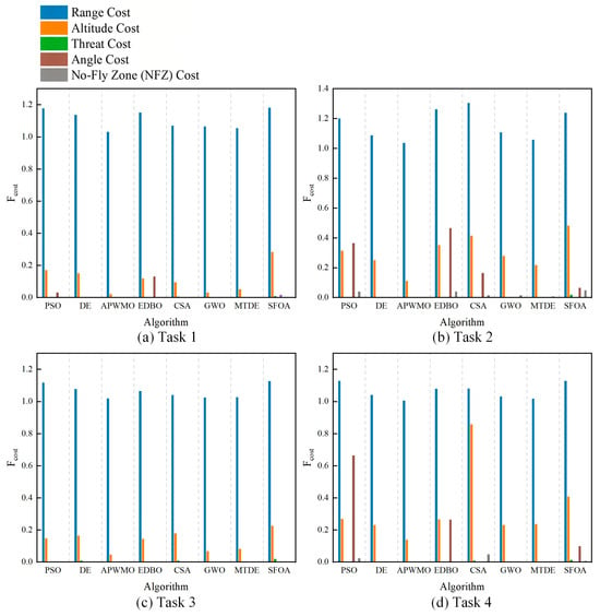
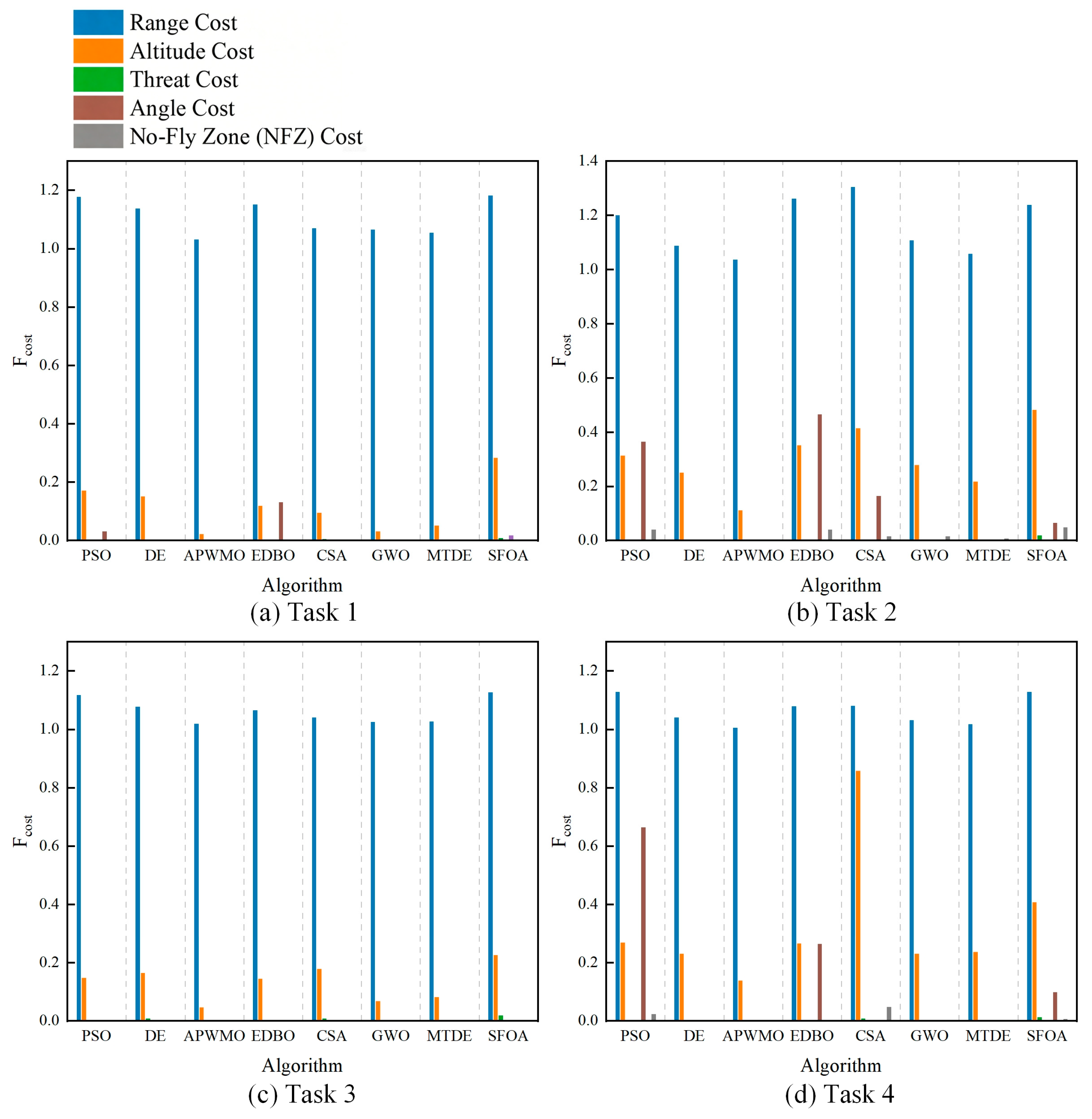

Disclaimer/Publisher’s Note: The statements, opinions and data contained in all publications are solely those of the individual author(s) and contributor(s) and not of MDPI and/or the editor(s). MDPI and/or the editor(s) disclaim responsibility for any injury to people or property resulting from any ideas, methods, instructions or products referred to in the content. |
© 2026 by the authors. Licensee MDPI, Basel, Switzerland. This article is an open access article distributed under the terms and conditions of the Creative Commons Attribution (CC BY) license.