Article

Predefined-Time Control for Automatic Carrier Landing Under Complex Wind Disturbances with Disturbance Observation and Prediction

1
College of Intelligent Systems Science and Engineering, Harbin Engineering University, Harbin 150001, China
2
China Ship Development and Design Center, Wuhan 430061, China
*
Author to whom correspondence should be addressed.
Drones 2026, 10(4), 308; https://doi.org/10.3390/drones10040308
Submission received: 23 March 2026 / Revised: 12 April 2026 / Accepted: 17 April 2026 / Published: 20 April 2026

Highlights

What are the main findings?
  • An active anti-disturbance control framework integrating predefined-time control, disturbance observation, and online disturbance prediction is proposed for automatic carrier landing under complex wind disturbances.
  • Simulation results show that the proposed method reduces the maximum following error by 16.9–82.0% and the touchdown error by 53.4–84.1%, compared with baseline methods.
What is the implication of the main findings?
  • The proposed method improves anti-disturbance capability and landing accuracy of carrier-based UAVs in composite wind environments, including airwake, steady wind, and gusts.

Abstract

To improve performance for automatic carrier landing under complex wind disturbances, an active anti-disturbance control method integrating predefined-time control, disturbance observation, and online disturbance prediction is proposed. A nonlinear model carrier-based unmanned aerial vehicle (UAV) under a composite wind environment, including airwake, steady wind, and gusts, is modeled. A predefined-time sliding mode controller is then developed to ensure that the system errors converge within a user-specified time. To enhance active anti-disturbance performance, a predefined-time disturbance observer is designed for disturbance estimation, and an online prediction method based on recursive least squares with forgetting factor is introduced to predict disturbances and mitigate the lag caused by observation and UAV dynamics. Moreover, a predefined-time reference model is incorporated to avoid the exponential explosion problem. Simulation results demonstrate that, compared with the baselines, the proposed method reduces the maximum following error by 16.9–82.0% and the touchdown error by 53.4–84.1%. These results indicate that the proposed method can effectively enhance anti-disturbance performance and landing accuracy under complex wind environments.

1. Introduction

Automic carrier landing for the UAV is recognized as one of the most challenging problems in flight control. Unlike conventional flight operations, carrier landings are characterized by a short operational window, rapid changes in UAV state, and stringent requirements for control precision. During approach and touchdown, the UAV must accurately adjust flight path, velocity, and attitude to satisfy strict safety and performance constraints [1]. Meanwhile, the UAV is subjected to strong aerodynamic disturbances induced by steady winds, gusts, and the airwake [2,3]. More broadly, wind disturbances not only affect flight stability and tracking accuracy, but may also influence UAV mission performance and endurance. Citroni et al. [4] analyzed the impact of wind conditions on the power consumption and mission performance of small UAVs, further highlighting the practical importance of studying UAV operation under aerodynamic disturbances. Therefore, developing an automatic carrier landing control (ACLS) with fast convergence, high path-following precision, and strong anti-disturbance capability remains crucial for carrier-based UAV [5].
Since carrier landing operations usually last only tens of seconds, the controller must rapidly eliminate system errors within the user-specified time. Therefore, nonlinear control methods with convergence time constraints have attracted increasing attention. Finite-time control ensures system states converge within a finite time, thereby offering faster error convergence than conventional asymptotic control methods. Fu et al. [6] developed a finite-time line-of-sight guidance law and controller to achieve high-precision path following under strong disturbances. As for carrier landing, Zhang et al. [7] incorporated finite-time control into the ACLS, enabling landing errors to converge within a finite time, thereby improving landing safety for the UAV. However, when the system’s initial conditions are unknown, it is difficult to determine the convergence time of finite-time control. Therefore, fixed-time control (FTC) was introduced to guarantee convergence within a bounded time independent of the initial condition. Liu et al. [8] developed an adaptive FTC for robotic trajectory tracking, which ensured convergence under arbitrary initial errors and improved both transient response and steady-state accuracy. In addition, Kumar et al. [9] proposed a robust wind-aware path-following guidance law for autonomous vehicles, which guarantees fixed-time convergence without explicit dependence on path curvature. Their study further demonstrates the importance of integrating fast convergence and explicit wind consideration into path-following control. Guan et al. [10] further applied FTC with disturbance observers to the ACLS, thus enabling the UAV to follow the desired landing path accurately. Nevertheless, in FTC, the upper bound of the convergence time is usually determined implicitly by multiple controller parameters. By contrast, predefined-time control (PTC) allows the convergence time bound to be explicitly introduced into the controller. Nguyen et al. [11] proposed a PTC for wheeled mobile robots subject to wheel slip and external disturbances. The results showed a significant improvement in trajectory tracking accuracy for both straight and U-shaped paths. In carrier landing, Li et al. [12] developed a PTC integrated with direct lift control (DLC), enabling the UAV to converge to the desired landing path within a predefined time under arbitrary initial error conditions, thus achieving predefined-time convergence of tracking errors under disturbances and improving landing accuracy.
In addition to rapid convergence, complex wind disturbances also degrade ACLS performance. Therefore, the ACLS based on sliding mode control (SMC) has been widely adopted for its robustness in suppressing disturbances. Yao et al. [13] proposed a global fast terminal sliding mode control method to improve the robustness of the ACLS. Similarly, Vilcica et al. [14] designed a robust SMC to mitigate model uncertainties and external disturbances. Considering the inherent chattering in conventional SMC, Yao et al. [15] further developed a super-twisting sliding mode control method that introduces an adaptive switching law. The method effectively reduced chattering and improved landing accuracy under airwake.
However, when disturbances are severe, time-varying, and persistent, robust feedback in SMC is weak to eliminate errors rapidly. This limitation has motivated the introduction of controllers with an observer. Observers estimate external disturbances and compensate them directly in the control law, thereby improving anti-disturbance performance. Yu et al. [16] designed a finite-time extended state observer for fixed-wing UAVs under external disturbances, demonstrating the effectiveness of observer-based disturbance compensation. For carrier landing, Yuan et al. [17] designed a backstepping controller with a disturbance observer to improve landing reliability under stochastic disturbances. Yao et al. [18] further proposed an active anti-disturbance control integrated with DLC, combining an extended state observer (ESO) to enhance landing accuracy and safety. In addition, Wu et al. [19] combined nonsingular terminal sliding mode control with ESO to simultaneously address actuator faults and external disturbances, thereby improving ACLS’s fault tolerance and trajectory tracking performance. However, the method does not guarantee convergence within a predefined time and does not explicitly consider the effects of severe and composite wind fields.
However, for fast time-varying disturbances, observers cannot compensate promptly. To further mitigate the lag of UAV dynamic regulation and observation estimation, several studies incorporate predictive information into the controller. Zhen et al. [20] developed an optimal preview control for UAVs by employing particle filtering to predict carrier deck motion online, and improve time-varying trajectory tracking performance. However, this method is mainly applicable to linear systems. Meng et al. [21] further incorporated neural-network-based airwake prediction into a model predictive controller, thereby improving anti-disturbance capability. However, this method relies on a large amount of disturbance data to train the neural network. Overall, studies on online short-term prediction and compensation of wind disturbances in carrier landing remain relatively scarce. Motivated by the above research, a predefined-time control method with disturbances observed and predicted is proposed. The main contributions of this work are summarized as follows.
  • A predefined-time sliding mode control method is developed for the ACLS. By introducing an explicit time parameter into the controller, the flight state errors are guaranteed to converge within a user-specified time, regardless of the initial conditions. Furthermore, a predefined-time reference model is incorporated into the ACLS to avoid the explosion of complexity in high-order systems while guaranteeing the system’s global predefined-time stability.
  • To enhance the active anti-disturbance performance of the ACLS, a predefined-time disturbance observer is designed to achieve rapid estimation of external disturbances. On this basis, an online short-term disturbance prediction method based on recursive least squares with a forgetting factor is proposed to predict the observed disturbances, thereby enhancing the effectiveness of ACLS in compensating for fast time-varying disturbances caused by airwake, steady wind, and gust.
The carrier-based UAV model and the composite wind environment are modeled in Section 2. Section 3 introduces the preliminaries related to controller design. In Section 4, the details of ACLS and the analysis of stability are presented. Section 5 reports the simulation results. Finally, Section 6 concludes this paper.

2. Problem Formulation

In this study, the carrier landing process is formulated as a path following problem. A six-degree-of-freedom (6-DOF) nonlinear UAV model and a composite wind model are established. Finally, the framework of the ACLS is described. A list of acronyms used in this paper is given in Appendix A.

2.1. Problem Statement

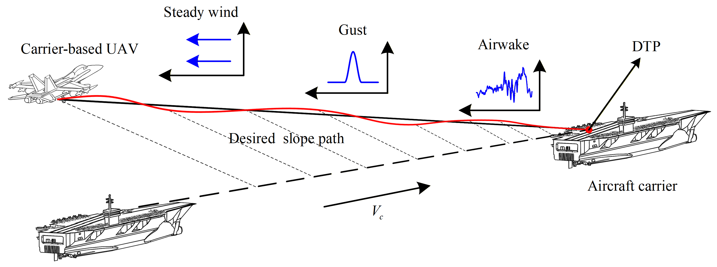
During carrier landing, successful arrestment requires the UAV to follow a desired slope path (DSP) with high precision while maintaining alignment with a predetermined area on the carrier deck. This predetermined area is referred to as the desired touchdown point (DTP), as described in Ref. [22]. Accordingly, the DSP is defined as a constant angle path terminating at the DTP. Moreover, the UAV is inevitably subjected to complex external wind disturbances during carrier landing. In this study, three wind disturbance components are considered: airwake, steady wind, and gust. Figure 1 shows the schematic of the carrier landing under complex wind disturbances. Therefore, the automatic carrier landing can be formulated as guiding and controlling the UAV to remain on the DSP in the presence of strong nonlinearities and external wind disturbances.

2.2. UAV Model

During carrier landing, the UAV is significantly affected by wind disturbances. As a result, conventional UAV models established under calm atmospheric conditions are no longer adequate for carrier landing. Therefore, this section presents the 6-DOF nonlinear dynamic and kinematic model of a UAV in the presence of wind disturbance [23,24,25], given by Equations (1)–(4).
x ˙ = V a cos χ cos γ + d x y ˙ = V a sin χ cos γ + d y h ˙ = V a sin γ + d h
V ˙ a = 1 m T cos α cos β + Y sin β D g sin γ + d V χ ˙ = cos μ m V a cos γ Y T cos α sin β + sin μ m V a cos γ L + T sin α + d χ γ ˙ = cos μ m V a L + T sin α sin μ m V a Y T cos α sin β g V a cos γ + d γ
α ˙ = q p cos α + r sin α tan β sec β γ ˙ cos μ + χ ˙ sin μ cos γ β ˙ = p sin α r cos α γ ˙ sin μ + χ ˙ cos μ cos γ μ ˙ = sec β p cos α + r sin α + γ ˙ tan β cos μ + χ ˙ sin γ + tan β sin μ cos γ
p ˙ = I 1 r + I 2 p q + I 3 L ¯ + I 4 N q ˙ = I 5 p r I 6 p 2 r 2 + I 7 M r ˙ = I 8 p I 2 r q + I 4 L ¯ + I 9 N
where m denotes the mass of the UAV, and g denotes the gravitational acceleration. [ x , y , h ] are the position coordinates of the UAV in the inertial reference frame, [ V a , γ , χ ] are the airspeed, the climb of angle (COA), and the heading angle, [ α , β , μ ] are the angle of attack (AOA), sideslip angle and roll angle of the UAV in the air reference frame, [ p , q , r ] are the angular rates in the body-fixed reference frame. [ Y , D , L ] , [ L ¯ , M , N ] , and T denote the UAV’s lateral, drag, and lift forces; roll, pitch, yaw moments; and engine thrust, respectively, as given in Equations (5) and (6). I i ( i = 1 , 2 , , 9 ) represent intermediate coefficients derived from the rotational inertias of UAV, and d i ( i = x , y , h , V , χ , γ ) denote external unknown disturbances caused by the wind, given in Appendix A.
L = C L 0 + C L α α + C L δ e δ e + C L δ f δ f q ¯ s D = C D 0 + C D α α + C D δ e δ e + C D δ f δ f q ¯ s Y = C Y 0 + C Y β β + C Y δ a δ a + C Y δ r δ r q ¯ s T = T max δ t
L ¯ = C l β β + C l p p b 2 V a + C l r r b 2 V a + C l δ a δ a + C l δ r δ r q ¯ s b M = C m 0 + C m α α + C m q q c 2 V a + C m δ e δ e + C m δ f δ f q ¯ s c ¯ N = C n β β + C n p p b 2 V a + C n r r b 2 V a + C n δ a δ a + C n δ r δ r q ¯ s b
where C i are aerodynamic coefficients. δ a , δ e , δ r , δ f , and δ t are the deflection angles of the aileron, elevator, rudder, flap, and throttle power, and these variables constitute the control inputs of the system. s, b, and c ¯ are the wing reference area, wingspan, and wing mean geometric chord. q ¯ is the dynamic pressure.
Assumption 1. 
The disturbances d i and their derivatives d ˙ i are bounded and continuous, satisfying d i < d ¯ i , d ˙ i < d ˙ ¯ i .
Remark 1. 
The UAV model established in Equations (1)–(4) is intended only for the normal flight envelope during the carrier landing, and it is not applicable to extreme conditions such as V a = 0 or γ = ± π 2 .
Assumption 2. 
All signals are assumed to be directly available, and measurement noise and measurement delays are not explicitly considered.

2.3. Airwake Model

Airwake is a critical environmental factor. The airwake model recommended in the flight quality standard MIL-F-8785C is widely adopted [26]. The airwake model consists of four components: free air turbulence, steady turbulence, periodic turbulence, and random turbulence [27], described by
u = u 1 + u 2 + u 3 + u 4 v = v 1 + v 4 w = w 1 + w 2 + w 3 + w 4
where u i , v i , and w i are the longitudinal, lateral and vertical airwake, i = 1 , 2 , 3 , 4 are the four components.

2.4. Steady Wind and Gust Model

During carrier landing, the UAV may operate under headwind or tailwind conditions with different wind speeds. The steady wind is defined as a wind field whose magnitude and direction remain constant over a given time interval, given as
V s = w c
where w c is the constant wind speed. In general, the steady wind acts primarily along the longitudinal direction and influences the UAV’s airspeed.
Moreover, gust disturbances may arise in the longitudinal, lateral, and vertical directions and impose more severe challenges on carrier landing because of their stronger, sharper variability and stochasticity [28]. Typical characteristics of gust include large amplitude fluctuations, short duration, and pronounced peak values. Accordingly, the gust model is adopted as
V g = V g p 2 1 cos 2 π T g t , 0 t T g 0 , e l s e
where V g p is the gust peak wind speed, and T g is the gust duration.
Assumption 3. 
Since this study focuses on carrier landing control under complex wind disturbances, deck motion during landing is not considered, thereby highlighting the performance of the proposed controller in suppressing wind disturbances.

2.5. Control Framework of the ACLS

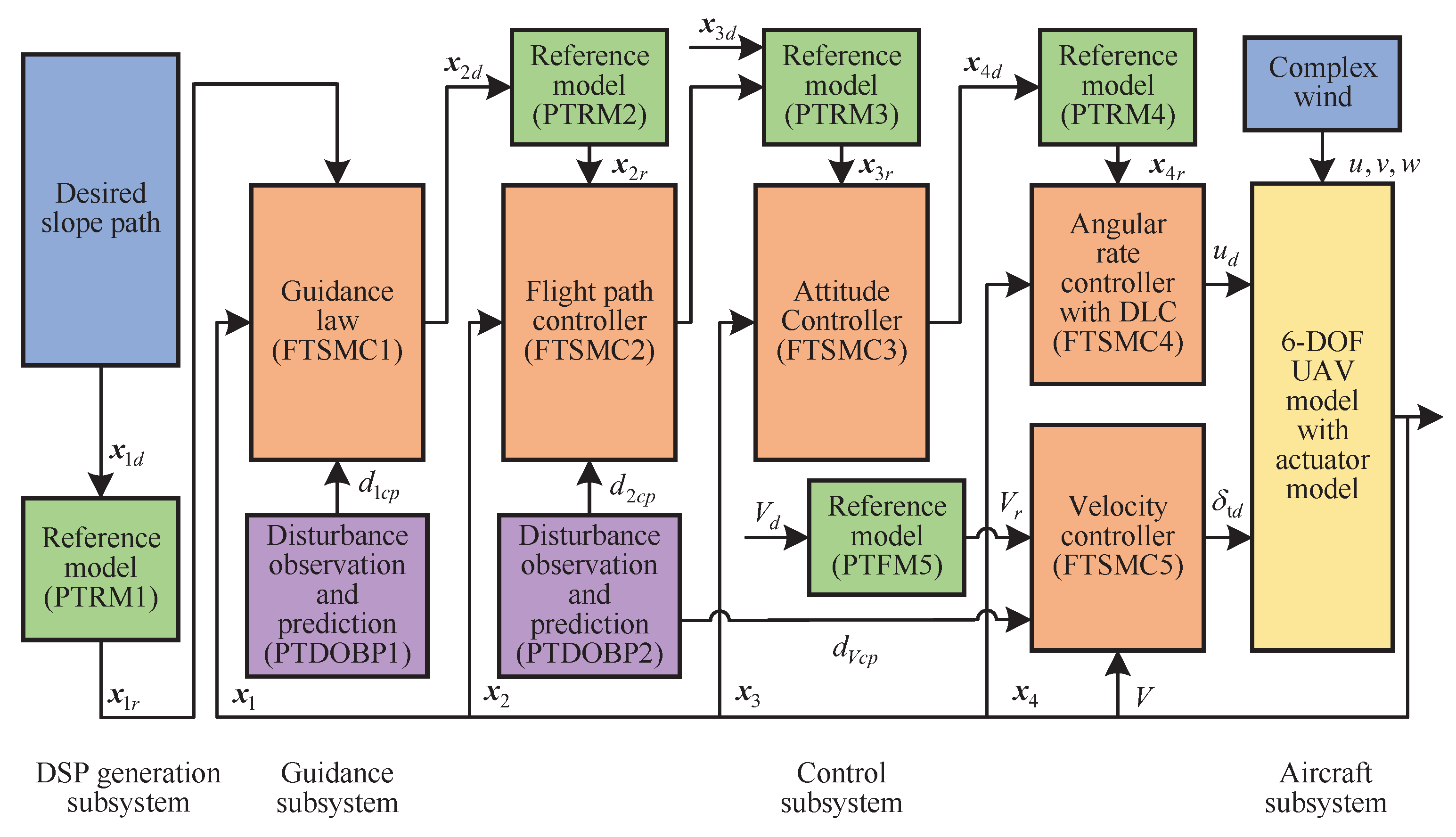
During carrier landing, the UAV is significantly affected by composite wind disturbances. To enhance the ACLS’s disturbance–rejection capability, a predefined-time control framework with disturbance observation and prediction is developed. The framework of the ACLS is illustrated in Figure 2. The ACLS consists of the reference models, disturbance observation and prediction, guidance law, heading angle controller, attitude controller, approach power compensation system, and angular rate controller with direct lift control.

3. Preliminaries

3.1. Nomenclature

Let R and R n denote the set of real numbers and the n-dimensional Euclidean space. For any matrix M , λ max ( M ) and λ min ( M ) denote the largest and smallest eigenvalues of M , respectively. Consider the nonlinear system
x ˙ = h ( t , x ) , h ( t , 0 ) = 0 , x R n
where x is the state vector, h ( t , x ) represents the nonlinear dynamics.
Lemma 1. 
([29]). For system (10), assume that there exists a radially unbounded Lyapunov function V whose derivative satisfies
V ˙ 2 ρ T p 2 V + V 1 ρ 2 + V 1 + ρ 2
where T p > 0 is the upper bound of the convergence time and ρ is a constant, ρ ( 0 , 1 ) . Then, the equilibrium of system (10) is predefined-time stable (PTS). Then the system state converges to the origin.
Lemma 2. 
([30]). For system (10), assume that there exists a radially unbounded Lyapunov function V satisfying
V ˙ 2 ρ T p 2 V + V 1 ρ 2 + V 1 + ρ 2 + Ω
where Ω is bounded. Then, system (10) is predefined-time stable, and T p is the upper bound of the convergence time. Furthermore, the system state converges to the residual set
lim t T p x | V ( x ) min 2 ρ T p Ω 2 2 , 2 ρ T p Ω 2 2 ρ , 2 ρ T p Ω 2 2 + ρ
Lemma 3. 
([31]). For any positive scalar ε and any scalar x R , the following inequality holds:
0 | x | x tanh x ε c ε ,
where c is a positive constant with c = 0.2785 .
Lemma 4. 
([32]). For any nonnegative real numbers x 1 , , x k , the following inequalities hold:
i = 1 k x i ρ 0 i = 1 k x i ρ 0 , 0 < ρ 0 < 1 , i = 1 k x i ρ 0 k 1 ρ 0 i = 1 k x i ρ 0 , ρ 0 > 1

3.2. Predefined-Time Reference Model

Conventional backstepping design for high-order nonlinear systems requires repeated differentiation of virtual control signals, which may lead to the “explosion of complexity” problem. Reference model and dynamic surface control are effective methods for alleviating this issue [24,33]. In this paper, a predefined-time reference model (PTRM) is developed to dynamically generate the reference signals and their derivatives within a predefined time. Let x d denote the desired signal, x ˙ d its derivative, and | x ˙ d | < x ˙ ¯ d . The proposed PTRM generates the reference signal x r and the derivative x ˙ r according to
x ˙ r = 2 2 ρ T r 2 + V r ρ 2 + V r ρ 2 e r + k r tanh e r ε
where k r > x ˙ ¯ d , e r = x d x r denotes the reference error, and the Lyapunov function is selected as V r = 1 2 e r T e r . Taking the time derivative of V r yields
V ˙ r = e r T e ˙ r = e r T x ˙ d e r T x ˙ r .
Substituting (15) into (16) yields
V ˙ r = e r T x ˙ d 2 ρ T r 2 V r + V r 1 ρ 2 + V r 1 + ρ 2 k r e r T tanh e r ε .
Since | x ˙ d | < x ˙ ¯ d and k r > x ˙ ¯ d , one has e r T x ˙ d i = 1 n | e r , i | x ˙ ¯ d k r i = 1 n | e r , i | .
By Lemma 3, it follows that
e r T x ˙ d k r i = 1 n c ε + e r , i tanh e r , i ε n k r c ε + k r e r T tanh e r ε .
where n denotes the dimension of the vector x . By defining Ω r = n k r c ε and combining (17) and (18), one obtains
V ˙ r 2 ρ T r 2 V r + V r 1 ρ 2 + V r 1 + ρ 2 + Ω r
According to Lemma 2, the proposed reference model in (15) is predefined-time stable, and V r converges to a small neighborhood of the origin within the predefined time T r .

3.3. Predefined-Time Disturbance Observer Design

To improve the anti-disturbance performance of the ACLS, a predefined-time disturbance observer (PTDOB) independent of state-derivative feedback is developed. Under the bounded condition in Assumption 1, the proposed observer drives the state estimation error into a small residual set within a predefined time and provides an effective disturbance approximation for compensation. Consider a general affine nonlinear system as follows:
x ˙ = f x + g x u + d
where x and u are the system state and input, d is the disturbance, f and g are the system nonlinear dynamics. For system (20), let x ^ denote the estimate of the state x . Let d ^ denote the estimate of the disturbance d , the observer dynamics and disturbance estimate are designed as
x ^ ˙ = f ( x ) + g ( x ) u + d ^ d ^ = 2 2 ρ T d 2 + V d ρ 2 + 14 ρ 2 V d ρ 2 x ˜ + k d tanh x ˜ ε
where k d > d ¯ , x ˜ = x x ^ is the state estimation error, and the Lyapunov function is chosen as V d = 1 2 x ˜ T x ˜ . Taking the time derivative of V d yields
V ˙ d = x ˜ T x ˜ ˙ = x ˜ T d x ˜ T d ^
By defining Ω d = n k d c ε and following the same procedure as in (17)–(19), one obtains
V ˙ d = x ˜ T d x ˜ T 2 2 ρ T d 2 + V d ρ 2 + 14 ρ 2 V d ρ 2 x ˜ + k d tanh x ˜ ε 2 ρ T d 2 V d + V d 1 ρ 2 + 14 ρ 2 V d 1 + ρ 2 + Ω d 2 ρ T d 2 V d + V d 1 ρ 2 + V d 1 + ρ 2 + Ω d
According to Lemma 2, under Assumption 1, the Lyapunov function V d converges to a small residual region within the predefined time T d . Hence, the state estimation error x ˜ is ultimately bounded and enters a small neighborhood of the origin within T d . For system (20), define the disturbance observation error as d ˜ = d d ^ = x ˙ x ^ ˙ = x ˜ ˙ . Therefore, d ^ provides an effective approximation of d for disturbance compensation, while the disturbance estimation error remains bounded and can be made sufficiently small [34].

3.4. Predefined-Time Sliding Mode Control

During carrier landing, to guarantee convergence of the DSP following error within a user-specified time while improving the robustness of the ACLS against external disturbances, a predefined-time sliding mode control (PTSMC) is developed for the system in (20). Define e = x d x and e ˙ = x ˙ d x ˙ = x ˙ d f x g x u d . The sliding surface is designed as
s = e + ϑ I
where ϑ I is an auxiliary integration variable, given as
ϑ ˙ I = ϑ = 2 2 ρ T c 2 + V e ρ 2 + V e ρ 2 e
V e is the Lyapunov function for error e , V e = 1 2 e T e . When the system reaches the sliding surface, s = 0 .
e = ϑ I
By taking the derivative of both sides of (26)
e ˙ = ϑ = 2 2 ρ T c 2 + V e ρ 2 + V e ρ 2 e
Then the time derivative of V e is
V ˙ e = e T e ˙ = 2 2 ρ T c 2 + V e ρ 2 + V e ρ 2 e T e 2 ρ T c 2 V e + V e 1 ρ 2 + V e 1 + ρ 2
According to Lemma 2, V e will converge to a small region around the origin, the residual set within T c .
The time derivative of Equation (24) is
s ˙ = e ˙ + ϑ = x ˙ d f gu d + ϑ
The control law is designed as
u = g 1 x ˙ d f d ^ + ϑ + 2 2 ρ T s 2 + V s ρ 2 + V s ρ 2 s + ks
where k = diag ( k 1 , k 2 , , k n ) , with k i is the positive constant. Substituting Equation (30) into Equation (29)
s ˙ = 2 2 ρ T s 2 + V s ρ 2 + V s ρ 2 s + k s + d ^ d = 2 2 ρ T s 2 + V s ρ 2 + V s ρ 2 s + k s d ˜
Define the Lyapunov function for sliding surface V s = 1 2 s T s , the time derivative of V s is
V ˙ s = s T s ˙ = s T 2 2 ρ T s 2 + V s ρ 2 + V s ρ 2 s + k s d ˜ = 2 ρ T s 2 V s + V s 1 ρ 2 + V s 1 + ρ 2 k s T s s T d ˜ 2 ρ T s 2 V s + V s 1 ρ 2 + V s 1 + ρ 2 k s T s + 1 4 s T s + d ˜ T d ˜ 2 ρ T s 2 V s + V s 1 ρ 2 + V s 1 + ρ 2 λ min ( k ) 1 4 s T s + d ˜ T d ˜
Selecting an appropriate value for k such that λ min ( k ) 1 4 > 0 and define Ω s = d ˜ T d ˜ , Equation (32) is modified as
V ˙ s 2 ρ T s 2 V s + V s 1 ρ 2 + V s 1 + ρ 2 + Ω s
According to Lemma 2, V s will converge to a small region around the origin within T s .

3.5. Disturbance Predictor

During carrier landing, the UAV is inevitably subjected to external disturbances caused by steady winds, gusts, and airwake in Section 2.3. Under severe sea conditions, these disturbances are characterized by large amplitudes, fast time-varying, and strong stochasticity, which significantly deteriorate the performance of the ACLS. In addition, there is an inherent lag in the UAV’s adjustment and disturbance estimation, which reduces the controller’s response speed and increases the following error. To further enhance the ACLS’s active anti-disturbance capability under complex wind conditions, a short-term disturbance prediction and compensation strategy is proposed. Specifically, the compensation signal is generated from the predicted PTDOB values and incorporated into the controllers as a feedforward term.
Since the temporal correlation of disturbance data, an autoregressive (AR) model is adopted to predict the observed disturbance values. The polynomial form in the AR model is given as [35]
d t + 1 = a 0 d ^ t + a 1 d ^ t 1 + a 2 d ^ t 2 + + a n d ^ t n + ϖ
where d ^ t i is the observed disturbance at the i -th time step before the current time step, and d t + 1 is the one-step predicted disturbance. a i is the AR coefficients to be identified, ϖ is zero-mean white noise. n denotes the model order, which is determined using the Bayesian Information Criterion (BIC). In this study, n = 5 .
During the carrier landing, the disturbances caused by wind vary rapidly, such that earlier observed data become less representative of the current disturbance. To improve prediction accuracy, a recursive least squares with forgetting factor λ (FFRLS) algorithm is employed to identify the AR model parameters online [36,37]. Define the parameter vector a t = [ a 0 , a 1 , , a n ] T and the state vector d ^ t = [ d ^ t , d ^ t 1 , , d ^ t n ] T , one has d t + 1 = a t T d ^ t + ϖ . The updated formulation in FFRLS is as follows:
  • Gain matrix update
    K t + 1 = p t d ^ t λ + d ^ t T p t d ^ t
  • Parameter vector update
    a t + 1 = a t + K t + 1 d ^ t + 1 a t T d ^ t
  • Covariance matrix update
    p t + 1 = 1 λ p t K t + 1 d ^ t T p t
Since an excessively short prediction horizon cannot provide sufficient information for disturbance compensation, whereas a longer horizon reduces prediction accuracy and increases computational complexity under rapidly varying disturbances, the subsequent 10 time steps are considered by balancing compensation effectiveness, prediction accuracy, and computational complexity. Furthermore, considering that the single-step disturbance predictions are uncertain, multiple predicted data are fused to construct a disturbance compensation signal d cp , defined as follows:
d cp = i = 1 10 w d i d t + i
where w d i is the weight coefficient corresponding to the prediction step. To effectively exploit multi-step predictions, confidence weights are assigned according to the prediction error variance, such that predictions with higher uncertainty make a smaller contribution to the compensation signal, given as
w d i = σ d i 2 j = 1 10 σ d j 2 , i = 1 , 2 , , 10 .
where σ d i 2 denotes the variance of the i-step prediction error. Therefore, a prediction step with a smaller error variance is assigned a larger weight, while a prediction step with higher uncertainty receives a smaller weight. In this way, short-term predictions with higher confidence contribute more to the disturbance compensation signal, whereas farther-step predictions with larger uncertainty are automatically suppressed. It is evident that this definition satisfies i = 1 10 w d i = 1 , w d i 0 . Based on this weighted formulation, the disturbance compensation signal is constructed as a linear combination of a finite number of predicted disturbance values. Therefore, if the predicted disturbances are bounded d t + i d ¯ , then the disturbance compensation signal d cp is also bounded. In fact, since the weights satisfy i = 1 10 w d i = 1 and w d i 0 , d cp is a convex combination of finitely many bounded predicted disturbances. The proof is given as
d cp = i = 1 10 w d i d t + i i = 1 10 w d i d t + i i = 1 10 w d i d ¯ d ¯ i = 1 10 w d i d ¯
Hence, the disturbance compensation signal remains bounded.
Remark 2. 
The disturbance compensation signal is employed as a surrogate for the unknown disturbance d in the system (20). Accordingly, the residual disturbance error is defined as d ˜ = d d c p . According to the stability analysis in (30)–(33), imperfect disturbance observation or prediction enters the closed-loop dynamics only through the bounded residual term Ω s . Since the residual disturbance error Ω s = d ˜ T d ˜ does not affect the closed-loop stability. Therefore, the proposed disturbance prediction and compensation method enhances active anti-disturbance in ACLS under complex wind disturbances while maintaining system PTS.

4. ACLS Design and Stability Analysis

This section provides the design of the ACLS and stability analysis. Considering the multi-time-scale characteristics of carrier-based UAV landing dynamics, singular perturbation theory is adopted as the theoretical basis for the slow–fast decomposition. The time-scale separation and singular perturbation theory have been recognized as effective tools for hierarchical control design of nonlinear systems, especially in the context of dynamic inversion for nonaffine-in-control systems [38]. In addition, existing automatic carrier landing studies commonly employ cascaded or hierarchical architectures, in which the control system is organized into guidance, attitude, angular-rate, and approach power compensation system (APCS) [14,27,39]. This architecture is consistent with the practical fact that position and lateral path dynamics evolve more slowly, whereas the attitude, angular-rate, and direct-lift-related channels respond faster under aerodynamic moments and control surface deflections. Therefore, the outer-loop variables are treated as slow dynamics, and the inner-loop variables are treated as fast dynamics, which facilitates systematic sub-controller design and reduces the coupling burden in the full-order nonlinear system. On this basis, the UAV model is rewritten in the affine nonlinear form in (41).
In conventional ACLS, flight path regulation is achieved indirectly through attitude control, which introduces inherent coupling between attitude and flight path dynamics, thereby limiting the ACLS’s response speed and control precision. To mitigate this problem, the DLC is introduced, and the COA is classified within the fast state. The flap generates lift to directly adjust the flight path angle without significantly impacting the UAV’s attitude. The flap generates lift to directly regulate the COA without significantly affecting the UAV attitude, and this mechanism has been widely recognized as effective for automatic carrier landing [40,41].
x ˙ 1 = f 1 x 2 , V a + g 1 V a x 2 + d 1 χ ˙ = f χ x 2 , x 3 , V a + g χ x 2 , x 3 , V a μ + d χ x ˙ 3 = f 3 x ˙ 2 , x 2 , x 3 + g 3 x 3 x 4 x ˙ 4 = f 4 x 3 , x 4 , V a + g 4 x 3 , V a u + d 4 V ˙ a = f V x 2 , x 3 + g V x 2 , x 3 δ t + d V
where x 1 = y , h T , x 2 = χ , γ T , x 3 = α , β , μ T , x 4 = γ , p , q , r T , u = δ f , δ a , δ e , δ r T . f i , g i , and d i are the nonlinear functions and the disturbance, provided in Appendix A. According to (41), the ACLS is organized into five interconnected sub-controllers: the guidance law, heading controller, attitude controller, angular rate controller with DLC, and approach power compensation system (APCS).

4.1. Guidance Law

During carrier landing, the UAV is required to follow the DSP and align with the DTP. The guidance law is designed to generate COA and heading angle commands from position errors. Specifically, the desired position is determined from the DTP, defined as x 1 d = y d h d T . Subsequently, the reference position x 1 r = y r h r T is generated by applying the generic PTRM introduced in Equation (15) of Section 3.2. Defining x ˙ ¯ 1 d is the upper bound of x ˙ 1 d , e 1 r is the reference model error, and e 1 r = x 1 d x 1 r . The PTRM is as follows
x ˙ 1 r = 2 2 ρ T 1 r 2 + V 1 r ρ 2 + 14 ρ 2 V 1 r ρ 2 e 1 r + k 1 r tanh e 1 r ε
where k 1 r > x ˙ ¯ 1 d , V 1 r is the Lyapunov function regarding e 1 r , and V 1 r = 1 2 e 1 r T e 1 r . Following (19), one has
V ˙ 1 r 2 ρ T 1 r 2 V 1 r + V 1 r 1 ρ 2 + 14 ρ 2 V 1 r 1 + ρ 2 + Ω 1 r
where Ω 1 r = 2 k 1 r c ε . Consider the position kinematics in (41)
x ˙ 1 = f 1 ( x 2 , V ) + g 1 ( V ) x 2 + d 1 .
Define the position error as e 1 = x 1 r x 1 . Then the position error dynamics satisfy
e ˙ 1 = x ˙ 1 r f 1 g 1 x 2 d 1 .
To achieve predefined-time convergence of the position error, the PTSMC in Section 3.4 is applied to system (44). The sliding variable s 1 for position error e 1 is defined as
s 1 = e 1 + ϑ I 1
where ϑ I 1 is an auxiliary integral state, defined as
ϑ ˙ I 1 = ϑ 1 = 2 2 ρ T 1 e 2 + V 1 e ρ 2 + V 1 e ρ 2 e 1
where V 1 e = 1 2 e 1 T e 1 is the Lyapunov function regarding position error e 1 .
According to Equation (30), the virtual control law is designed as
x 2 d = g 1 1 x ˙ 1 r f 1 d 1 cp + ϑ 1 + 2 2 ρ T 1 s 2 + V 1 s ρ 2 + 14 ρ 2 V 1 s ρ 2 s 1 + k 1 s 1
where d 1 cp is the compensation value generated by the predefined-time disturbance observer and predictor (PTDOBP) in Section 3.3 and Section 3.5, and d ˜ 1 = d 1 d 1 cp denotes the disturbance compensation error.
Choose the Lyapunov function regarding the sliding variable s 1 as V 1 s = 1 2 s 1 T s 1 . Then, similar to (32) and (33), by defining Ω 1 s = d ˜ 1 T d ˜ 1 , the time derivative of V 1 s satisfies
V ˙ 1 s 2 ρ T 1 s 2 V 1 s + V 1 s 1 ρ 2 + 14 ρ 2 V 1 s 1 + ρ 2 + Ω 1 s
Remark 3. 
The coefficient 14 ρ 2 is introduced here for consistency with the global stability analysis in Section 4.6. Since 14 Lyapunov components are aggregated there, this factor compensates for the scaling term generated by Lemma 4 when handling j = 1 14 V j 1 + ρ 2 . The coefficient 14 ρ 2 appearing subsequently is introduced for the same reason.

4.2. Heading Angle Control

In the ACLS, the heading angle controller is designed to drive the UAV heading to track the heading angle commands generated by the guidance law. Specifically, the guidance commands serve as the controller input, whereas the corresponding output is the roll angle commands. To avoid the complexity caused by directly differentiating the guidance signals, the reference heading angle χ r and the derivative χ ˙ r for the UAV are generated through the PTRM introduced in Section 3.2, Defining χ ˙ ¯ d is the upper bound of χ ˙ d , e 2 r is the reference model error, and e 2 r = χ d χ r . The PTRM is expressed as follows:
χ ˙ r = 2 2 ρ T 2 r 2 + V 2 r ρ 2 + 14 ρ 2 V 2 r ρ 2 e 2 r + k 2 r tanh e 2 r ε
where k 2 r > χ ˙ ¯ d , V 2 r is the Lyapunov function regarding e 2 r , V 2 r = 1 2 e 2 r T e 2 r . Following (19), one has
V ˙ 2 r 2 ρ T 2 r 2 V 2 r + V 2 r 1 ρ 2 + 14 ρ 2 V 2 r 1 + ρ 2 + Ω 2 r
where Ω 2 r = k 2 r c ε . Consider the heading angle kinematics in (41)
χ ˙ = f χ x 2 , x 3 , V + g χ x 2 , x 3 , V μ + d χ
Define the heading angle error as e 2 r = χ r χ , and the heading angle error dynamics satisfy
e ˙ 2 = χ ˙ r f χ g χ μ d χ
To achieve predefined-time convergence of the heading angle error, the PTSMC described in Section 3.4 is applied to system (52). The corresponding sliding variable s 2 for the heading angle error e 2 is defined as
s 2 = e 2 + ϑ I 2
where ϑ I 2 is an auxiliary integral state, defined as
ϑ ˙ I 2 = ϑ 2 = 2 2 ρ T 2 e 2 + V 2 e ρ 2 + V 2 e ρ 2 e 2
where V 2 e = 1 2 e 2 T e 2 is the Lyapunov function regarding heading angle error e 2 .
According to Equation (30), the virtual control law is designed as
μ d = g χ 1 x ˙ χ r f χ d χ cp + ϑ 2 + 2 2 ρ T 2 s 2 + V 2 s ρ 2 + 14 ρ 2 V 2 s ρ 2 s 2 + k 2 s 2
where d χ cp is the compensation value generated by the PTDOBP in Section 3.3 and Section 3.5, and d ˜ χ = d ^ χ d χ cp denotes the disturbance compensation error.
Choose the Lyapunov function for the sliding variable s 2 as V 2 s = 1 2 s 2 T s 2 . Then, similar to (32) and (33), by defining Ω 2 s = d ˜ χ T d ˜ χ , the time derivative of V 2 s satisfies
V ˙ 2 s 2 ρ T 2 s 2 V 2 s + V 2 s 1 ρ 2 + 14 ρ 2 V 2 s 1 + ρ 2 + Ω 2 s

4.3. Attitude Control

During carrier landing, since the UAV operates under low dynamic pressure, maintaining aerodynamic attitude stability is essential. The AOA and sideslip angle are required to maintain their nominal values, α d = 8.1 ° and β d = 0 ° . In the ACLS, the attitude controller is responsible for regulating the AOA, sideslip angle, and roll angle according to the desired attitude command x 3 d = α d β d μ d T . The input to the attitude controller is the desired attitude angle commands, whereas its output is the corresponding angular rate command. To avoid the complexity caused by directly differentiating the desired attitude angle x 3 d , the reference attitude angle x 3 r and the derivative x ˙ 3 r for the UAV are generated by the PTRM introduced in Section 3.2. Defining x ˙ ¯ 3 d is the upper bound of x ˙ 3 d , e 3 r is the reference model error, and e 3 r = x 3 d x 3 r . The PTRM is expressed as follows:
x ˙ 3 r = 2 2 ρ T 3 r 2 + V 3 r ρ 2 + 14 ρ 2 V 3 r ρ 2 e 3 r + k 3 r tanh e 3 r ε
where k 3 r > x ˙ ¯ 3 d , V 3 r is the Lyapunov function regarding e 3 r , V 3 r = 1 2 e 3 r T e 3 r . Following (19), one has
V ˙ 3 r 2 ρ T 3 r 2 V 3 r + V 3 r 1 ρ 2 + 14 ρ 2 V 3 r 1 + ρ 2 + Ω 3 r
where Ω 2 r = k 2 r c ε . Consider the attitude dynamic in system (41),
x ˙ 3 = f 3 x ˙ 2 , x 2 , x 3 + g 3 x 3 x 4
Define the attitude angle error as e 3 = x 3 r x 3 . Then, the dynamics can be written as
e ˙ 3 = x ˙ 3 r f 3 g 3 x 4
To achieve predefined-time convergence of the attitude angle error, the PTSMC described in Section 3.4 is applied to system (60). The corresponding sliding variable s 3 for the attitude angle error e 3 is defined as
s 3 = e 3 + ϑ I 3
where ϑ I 3 is an auxiliary integral state, defined as
ϑ ˙ I 3 = ϑ 3 = 2 2 ρ T 3 e 2 + V 3 e ρ 2 + V 3 e ρ 2 e 3
where V 3 e = 1 2 e 3 T e 3 is the Lyapunov function regarding attitude angle error e 3 .
According to Equation (30), the virtual control law is designed as
x 4 d = g 3 1 x ˙ 3 r f 3 + ϑ 3 + 2 2 ρ T 3 s 2 + V 3 s ρ 2 + 14 ρ 2 V 3 s ρ 2 s 3 + k 3 s 3
Choose the Lyapunov function for the sliding variable s 3 as V 3 s = 1 2 s 3 T s 3 . Then, similar to Equations (32) and (33), the time derivative of V 3 s satisfies
V ˙ 3 s 2 ρ T 3 s 2 V 3 s + V 3 s 1 ρ 2 + 14 ρ 2 V 3 s 1 + ρ 2
According to the adopted model in Equations (3) and (41), the attitude subsystem (60) does not include an explicit disturbance term. Therefore, no disturbance observer is designed for this controller, and only V 3 r and V 3 s are involved in the Lyapunov analysis of the attitude sub-controller. This will affect the number of terms in Equations (82) and (83).

4.4. Angular Rate Control with DLC

The angular rate controller with DLC is designed to regulate the UAV’s angular rates and the COA according to the desired command x 4 d . Its input consists of the desired angular rate and COA signals, while its output is the corresponding deflection commands for the aileron, elevator, rudder, and flap. To avoid the complexity caused by directly differentiating the desired signal x 4 d , the reference attitude angle x 4 r and the derivative x ˙ 4 r for the UAV are generated by the PTRM introduced in Section 3.2. Defining x ˙ ¯ 4 d is the upper bound of x ˙ 4 d , e 4 r is the reference model error, and e 4 r = x 4 d x 4 r . The PTRM is expressed as follows:
x ˙ 4 r = 2 2 ρ T 4 r 2 + V 4 r ρ 2 + 14 ρ 2 V 4 r ρ 2 e 4 r + k 4 r tanh e 4 r ε
where k 4 r > x ˙ ¯ 4 d , V 4 r is the Lyapunov function regarding e 4 r , and V 4 r = 1 2 e 4 r T e 4 r . According to (19), one has
V ˙ 4 r 2 ρ T 4 r 2 V 4 r + V 4 r 1 ρ 2 + 14 ρ 2 V 4 r 1 + ρ 2 + Ω 4 r
where Ω 4 r = 4 k 4 r c ε . Consider the angular rate kinematics of the UAV in system (41)
x ˙ 4 = f 4 x 3 , x 4 , V + g 4 x 3 , V u + d 4
Define the angular rate error as e 4 = x 4 r x 4 , Then the dynamics satisfy
e ˙ 4 = x ˙ 4 r f 4 g 4 u d 4 .
To achieve predefined-time convergence of the angular rate tracking error, the PTSMC developed in Section 3.4 is applied to system (68). The corresponding sliding variable s 4 for the angular rate error e 4 is defined as
s 4 = e 4 + ϑ I 4
where ϑ I 4 is an auxiliary integral state, defined as
ϑ ˙ I 4 = ϑ 4 = 2 2 ρ T 4 e 2 + V 4 e ρ 2 + 14 ρ 2 V 4 e ρ 2 e 4
where V 4 e = 1 2 e 4 T e 4 is the Lyapunov function regarding angular rate error e 4 .
According to Equation (30), the virtual control law is designed as
u d = g 4 1 x ˙ 4 r f 4 d 4 cp + ϑ 4 + 2 2 ρ T 4 s 2 + V 4 s ρ 2 + 14 ρ 2 V 4 s ρ 2 s 4 + k 4 s 4
where d 4 cp is the compensation value generated by the PTDOBP in Section 3.3 and Section 3.5, and d ˜ 4 = d 4 d 4 cp denotes the disturbance compensation error.
Choose the Lyapunov function candidate for the sliding variable s 4 as V 4 s = 1 2 s 4 T s 4 .
Then, similar to (32) and (33), by defining Ω 4 s = d ˜ 4 T d ˜ 4 , the time derivative of V 4 s satisfies
V ˙ 4 s 2 ρ T 4 s 2 V 4 s + V 4 s 1 ρ 2 + 14 ρ 2 V 4 s 1 + ρ 2 + Ω 4 s

4.5. Approach Power Compensation System

The APCS in the ACLS is designed to regulate the UAV velocity during the approach phase. The input to the APCS is the desired velocity command, V d = 70 m / s , whereas its output is the throttle command. To avoid the complexity caused by directly differentiating the desired signal V d , the reference velocity V r and the derivative V ˙ r for the UAV are generated by the PTRM introduced in Section 3.2. Defining V ˙ ¯ d is the upper bound of V ˙ d , e 5 r is the reference model error, and e 5 r = V d V r . The PTRM is expressed as follows:
V ˙ r = 2 2 ρ T 5 r 2 + V 5 r ρ 2 + 14 ρ 2 V 5 r ρ 2 e 5 r + k 5 r tanh e 5 r ε
where k 5 r > V ˙ ¯ d , and the associated Lyapunov function is chosen as V 5 r = 1 2 e 5 r T e 5 r . According to (19), one obtains
V ˙ 5 r 2 ρ T 5 r 2 V 5 r + V 5 r 1 ρ 2 + 14 ρ 2 V 5 r 1 + ρ 2 + Ω 5 r
where Ω 5 r = k 5 r c ε . Consider the velocity dynamic model in system (41)
V ˙ 5 = f V x 2 , x 3 + g V x 2 , x 3 δ t + d V
Define the velocity error as e 5 = V r V a , then the velocity error dynamics satisfy
e ˙ 5 = V ˙ r f V g V δ t d V .
To achieve predefined-time convergence of the velocity tracking error, the PTSMC developed in Section 3.4 is applied to system (76). The corresponding sliding variable s 5 for the velocity error e 5 is defined as
s 5 = e 5 + ϑ I 5
where ϑ I 5 is an auxiliary integral state, defined as
ϑ ˙ I 5 = ϑ 5 = 2 2 ρ T 5 e 2 + V 5 e ρ 2 + 14 ρ 2 V 5 e ρ 2 e 5
where V 5 e = 1 2 e 5 T e 5 is the Lyapunov function regarding velocity error e 5 .
According to Equation (30), the virtual control law is designed as
δ t d = g V 1 x ˙ 5 r f V d V cp + ϑ 5 + 2 2 ρ T 5 s 2 + V 5 s ρ 2 + 14 ρ 2 V 5 s ρ 2 s 5 + k 5 s 5
where d V cp is the compensation value generated by the PTDOBP in Section 3.3 and Section 3.5, and d ˜ V = d V d V cp denotes the disturbance compensation error.
Choose the Lyapunov function regarding the sliding variable s 5 as V 5 s = 1 2 s 5 T s 5 . Then, similar to (32) and (33), by defining Ω 5 s = d ˜ V T d ˜ V , the time derivative of V 5 s satisfies
V ˙ 5 s 2 ρ T 5 s 2 V 5 s + V 5 s 1 ρ 2 + 14 ρ 2 V 5 s 1 + ρ 2 + Ω 5 s

4.6. Stability Analysis

Theorem 1. 
For the UAV model under complex wind disturbances, suppose that Assumptions 1–3 hold. If the proposed PTRM, PTDOBP, and PTSMC are integrated into the ACLS, then, for any initial error conditions, all signals are ultimately bounded, and the state errors converge within a predefined time.
Proof of Theorem 1. 
The global Lyapunov function for the ACLS is defined as V g = i = 1 5 V i s + V i r + V i d . Combining Equations (23), (43), (49), (51), (57), (59), (65), (67), (73), (75) and (81), the time derivative of V g is obtained as
V ˙ g = i = 1 5 V ˙ i s + V ˙ i r + V ˙ i d i = 1 5 [ 2 ρ T i s 2 V i s + V i s 1 ρ 2 + 14 ρ 2 V i s 1 + ρ 2 2 ρ T i r 2 V i r + V i r 1 ρ 2 + 14 ρ 2 V i r 1 + ρ 2 2 ρ T i d 2 V i d + V i d 1 ρ 2 + 14 ρ 2 V i d 1 + ρ 2 + Ω i s + Ω i r + Ω i d ]
By defining T g = max T i s , T i r , T i d , Ω g = i = 1 5 Ω i s + Ω i r + Ω i d , one has
V ˙ g j = 1 14 2 ρ T g 2 V j + V j 1 ρ 2 + 14 ρ 2 V j 1 + ρ 2 + Ω g
where { V j } j = 1 14 represents the set of all Lyapunov components { V i s , V i r , V i d } i = 1 5 . By Lemma 4, it follows that
V ˙ g 2 ρ T g 2 j = 1 14 V j + j = 1 14 V j 1 ρ 2 + 14 ρ 2 j = 1 14 V j 1 + ρ 2 + Ω g 2 ρ T g 2 j = 1 14 V j + j = 1 14 V j 1 ρ 2 + j = 1 14 V j 1 + ρ 2 + Ω g 2 ρ T g 2 V g + V g 1 ρ 2 + V g 1 + ρ 2 + Ω g
According to Lemma 2, for any admissible initial condition satisfying the assumptions, all signals remain ultimately bounded, and the system errors enter the residual set S g = lim t T p x | V g ( x ) min 2 ρ T g Ω g 2 2 , 2 ρ T g Ω g 2 2 ρ , 2 ρ T g Ω g 2 2 + ρ within the predefined time T g and remain therein thereafter. Then the proof is completed. □

5. Simulations

In this section, simulation experiments are conducted to validate the effectiveness and superiority of the proposed control method. First, the simulation framework settings are introduced. Then, two sets of experiments are considered. In Experiment 1, ideal operating conditions without external disturbances are assumed to verify that the proposed control method drives the flight states to converge within a prescribed time for different initial errors. In Experiment 2, the performance of the proposed control method is evaluated under a composite disturbance environment consisting of airwake, steady wind, and gusts. The proposed predefined-time control with disturbance observer and prediction (PTC-DOBP) is compared with three baseline methods: FTC, predefined-time control (PTC), and predefined-time control with disturbance observer (PTC-DOB).

5.1. Simulation Conditions

To validate the proposed method, simulations are conducted on a semi-physical simulation platform that supports real-time execution, data logging, three-dimensional visualization, and human–machine interaction, thereby enabling a high-fidelity automatic carrier landing process under wind disturbances. The platform integrates the six-DOF UAV model described in Section 2.2 and Section 2.3 and the composite wind disturbance model presented in Section 2.3. The nominal landing conditions of the UAV, the carrier parameters, the actuator dynamics, and control limits of the flaps, ailerons, elevators, and rudder are listed in Appendix A. These settings are kept identical across all comparative simulations. The engine model adopted in this study is given as
δ t δ td = 2.994 s 3 + 3.5 s 2 + 9.18 s + 3.13 s 4 + 6.5 s 3 + 18.25 s 2 + 26.28 s + 9.37
In the closed-loop simulation, the actuator commands u d and the throttle command δ td in Equations (72) and (80) are not applied directly to the UAV model. Instead, they are first passed through the actuator dynamics and engine dynamics described in Table A2 and Equation (85), which produce the actual actuator response u and the actual throttle response δ t . The resulting actuator response and throttle response are then used in the force and moment model of the UAV in (5) and (6).
The predefined-time parameters are chosen based on the slow-fast time-scale separation of the carrier-based UAV dynamics, with larger values for the outer-loop slow subsystems and smaller values for the inner-loop fast subsystems. Moreover, the predefined-time parameters of the PTRMs and PTDOBs are set to be smaller than those of the controllers, to ensure faster reference generation and disturbance estimation. The main design parameters of ACLS are as follows: ρ = 0.4 , for the controller: T 1 s = [ 12 , 10 ] , T 2 s = 8 , T 3 s = [ 6 , 6 , 6 ] , T 4 s = [ 6 , 4 , 4 , 4 , 4 ] , T 5 s = 8 . for the PTRMs and PTDOBs, the following values are uniformly selected: T i r = T i d = 3 .

5.2. Experiment 1

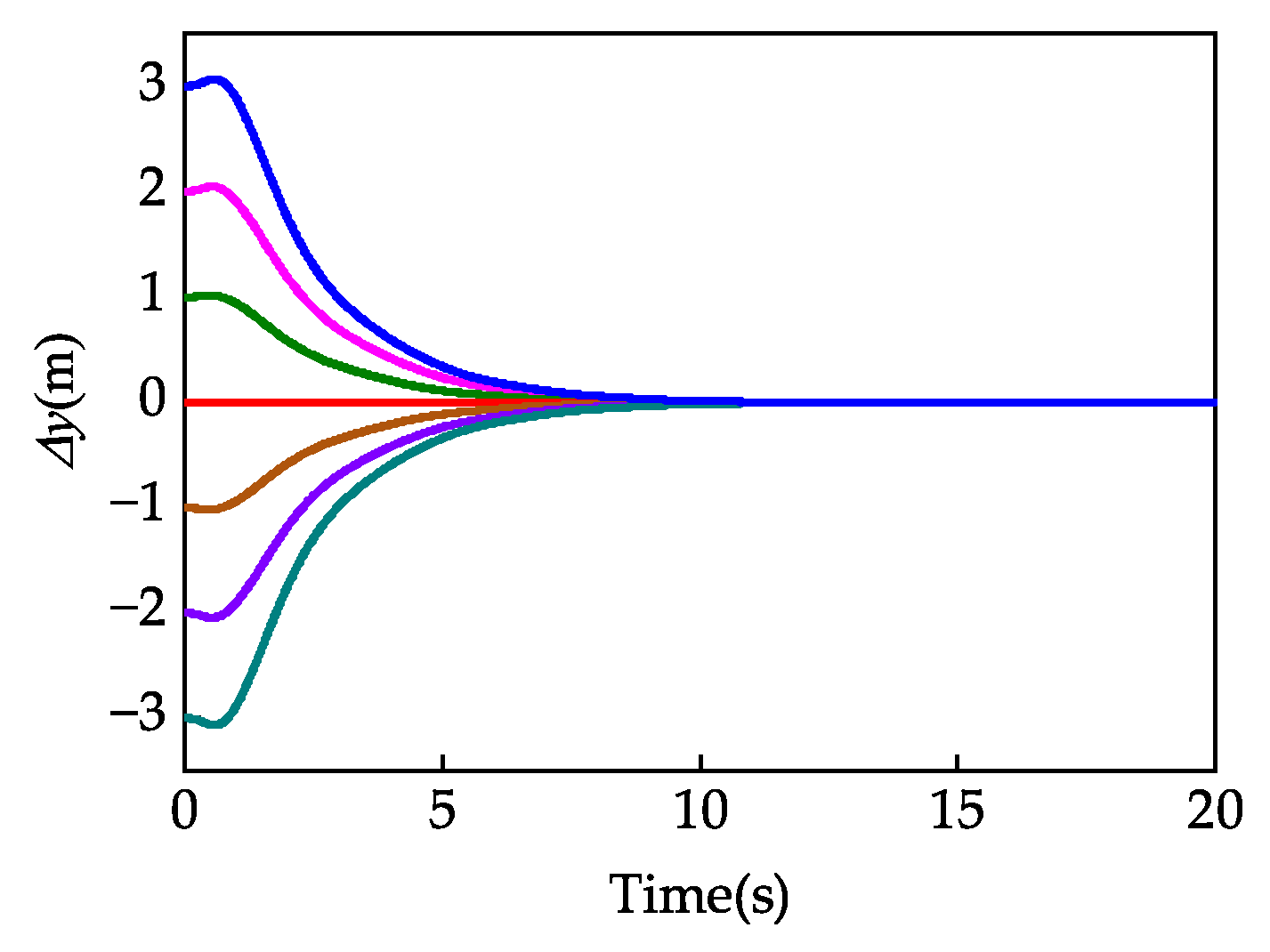
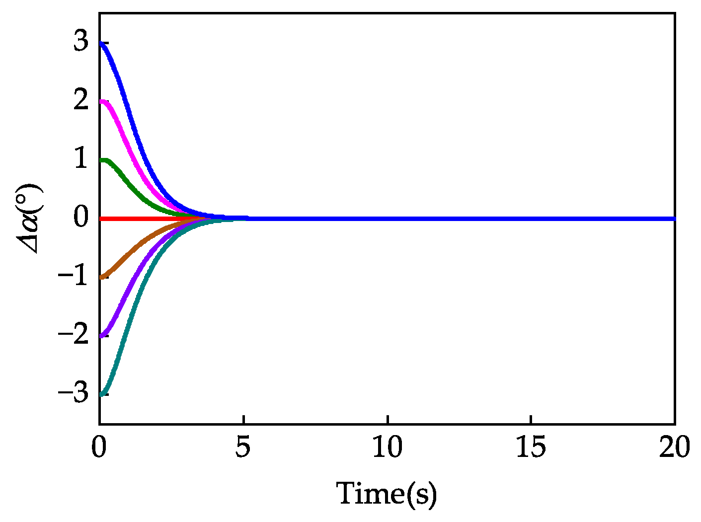
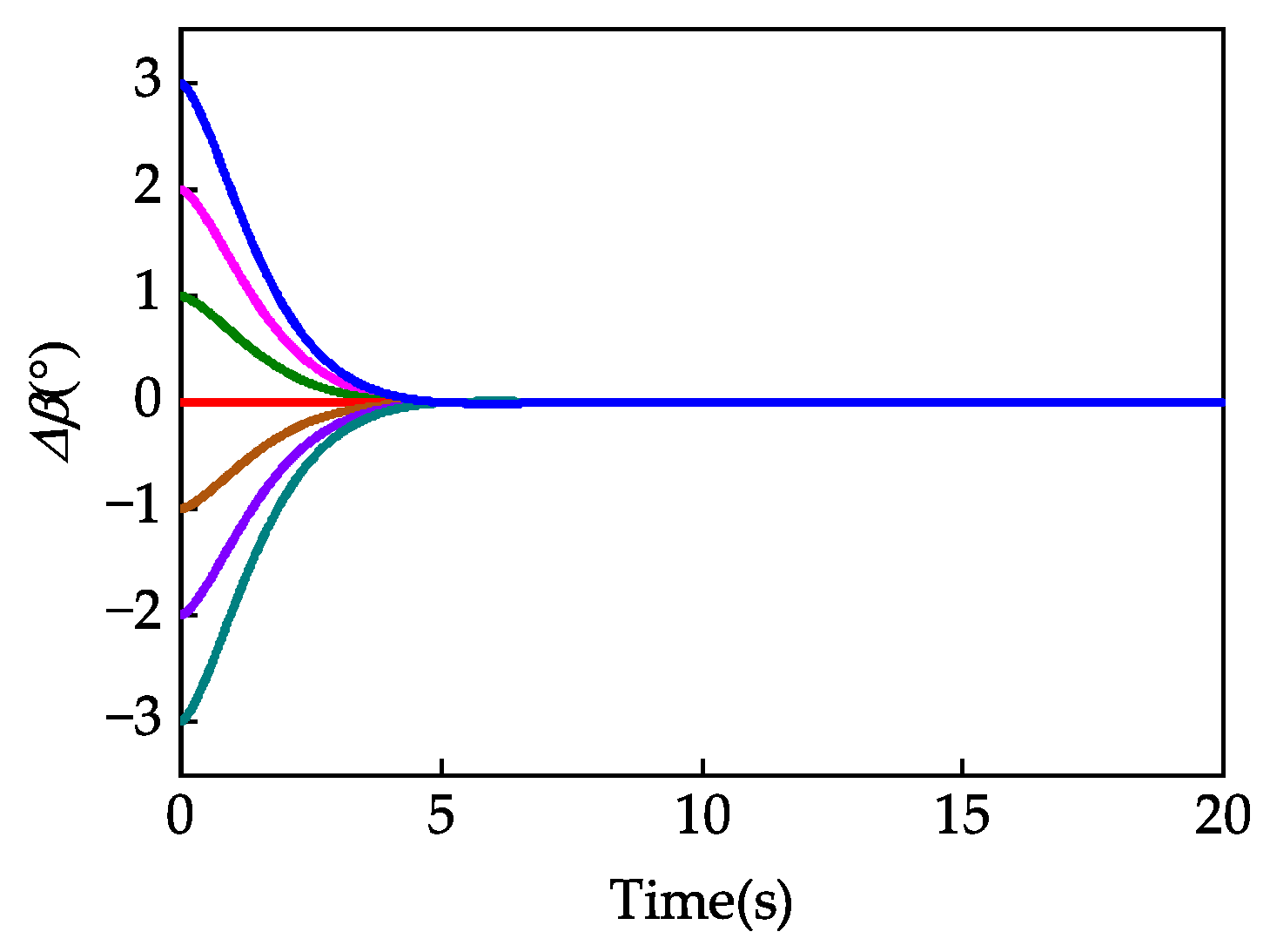
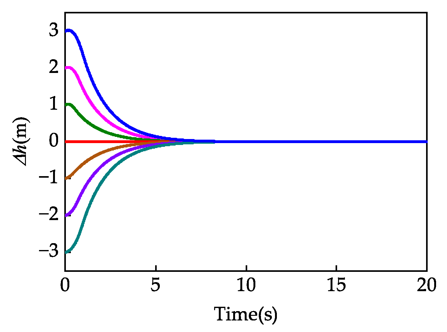
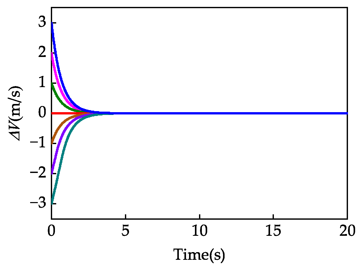
This section verifies the predefined-time convergence property of the proposed controller under no disturbance conditions. Different initial errors are introduced into the altitude, lateral position, velocity, AOA, and sideslip angle. For each state, the initial error is uniformly varied over the interval [ 3 , 3] with a step size of 1. The corresponding error responses are shown in Figure 3, Figure 4, Figure 5, Figure 6 and Figure 7.
The results indicate that, under ideal conditions, the altitude, lateral position, velocity, AOA, and sideslip angle errors all converge within their predefined times under the proposed method. Specifically, the altitude and lateral position errors converge within 10 s and 12 s, respectively (Figure 3 and Figure 4), whereas the velocity, AOA, and sideslip angle errors converge within 5 s (Figure 5, Figure 6 and Figure 7). These results verify that the proposed method achieves predefined-time stabilization under different initial conditions. The differences in convergence time are mainly attributed to the inherent timescale separation of the UAV dynamics. The altitude and lateral position errors are the outer-loop position states with relatively slow dynamics. Therefore, longer predefined convergence times are adopted to avoid overly aggressive control actions. In contrast, the velocity, AOA, and sideslip angle states belong to the inner-loop fast dynamics and possess a higher dynamic bandwidth. In addition, the DLC accelerates vertical flight path correction by directly adjusting lift, thereby improving altitude regulation performance and enhancing disturbance rejection in complex wind environments.
Remark 4. 
The predefined-time parameter specifies only an upper bound on the convergence time, and the actual convergence is generally achieved in a shorter time. Therefore, the predefined time should not be chosen excessively small. Otherwise, excessively stringent convergence requirements may require overly large control gains, leading to actuator saturation and degraded control performance. In extreme cases, such a setting may even exceed the system’s achievable performance and compromise closed-loop stability.

5.3. Experiment 2

To evaluate the superiority of the proposed PTC-DOBP method for automatic carrier landing under wind disturbances, the path-following error and anti-disturbance performance of four methods—FTC, PTC, PTC-DOB, and PTC-DOBP—are comprehensively compared. The PTC, PTC-DOB, and PTC-DOBP methods adopt the same PTRM and PTSMC. In addition, PTC-DOB enhances the baseline controller by integrating the PTDOB presented in Section 3.2, while PTC-DOBP further incorporates the disturbance prediction module introduced in Section 3.4.
The composite wind disturbance consists of airwake, steady wind, and gust components. The airwake is modeled using four components and exerts the most significant influence on the carrier stern. The steady wind is along the longitudinal direction to represent a constant headwind or tailwind at 10 m/s. In addition, gusts with a max magnitude of 4 m/s are introduced along the longitudinal, lateral, and vertical directions. The initial longitudinal distance between the UAV and the carrier is set to 2056.2 m, and the initial altitude is 147 m. The initial altitude and lateral position errors are both set to 1 m. The total simulation duration is 30 s.
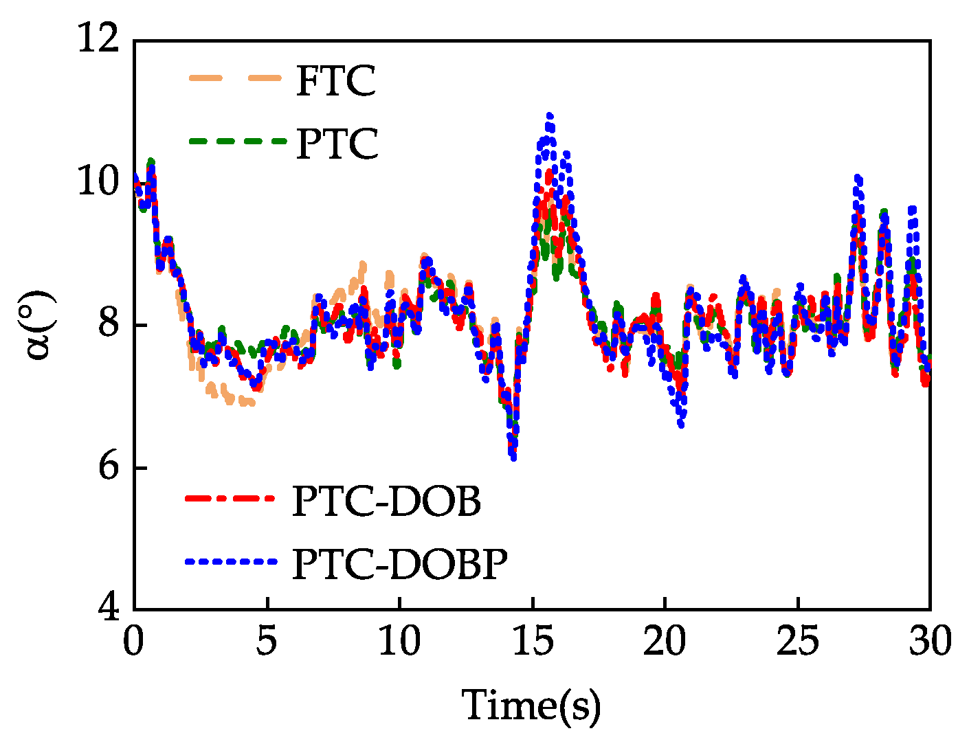
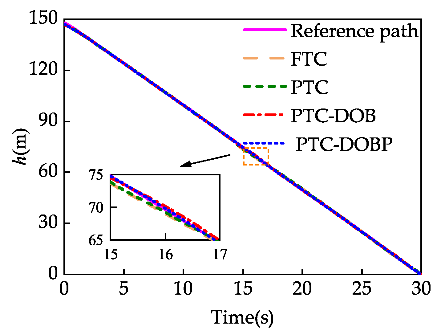
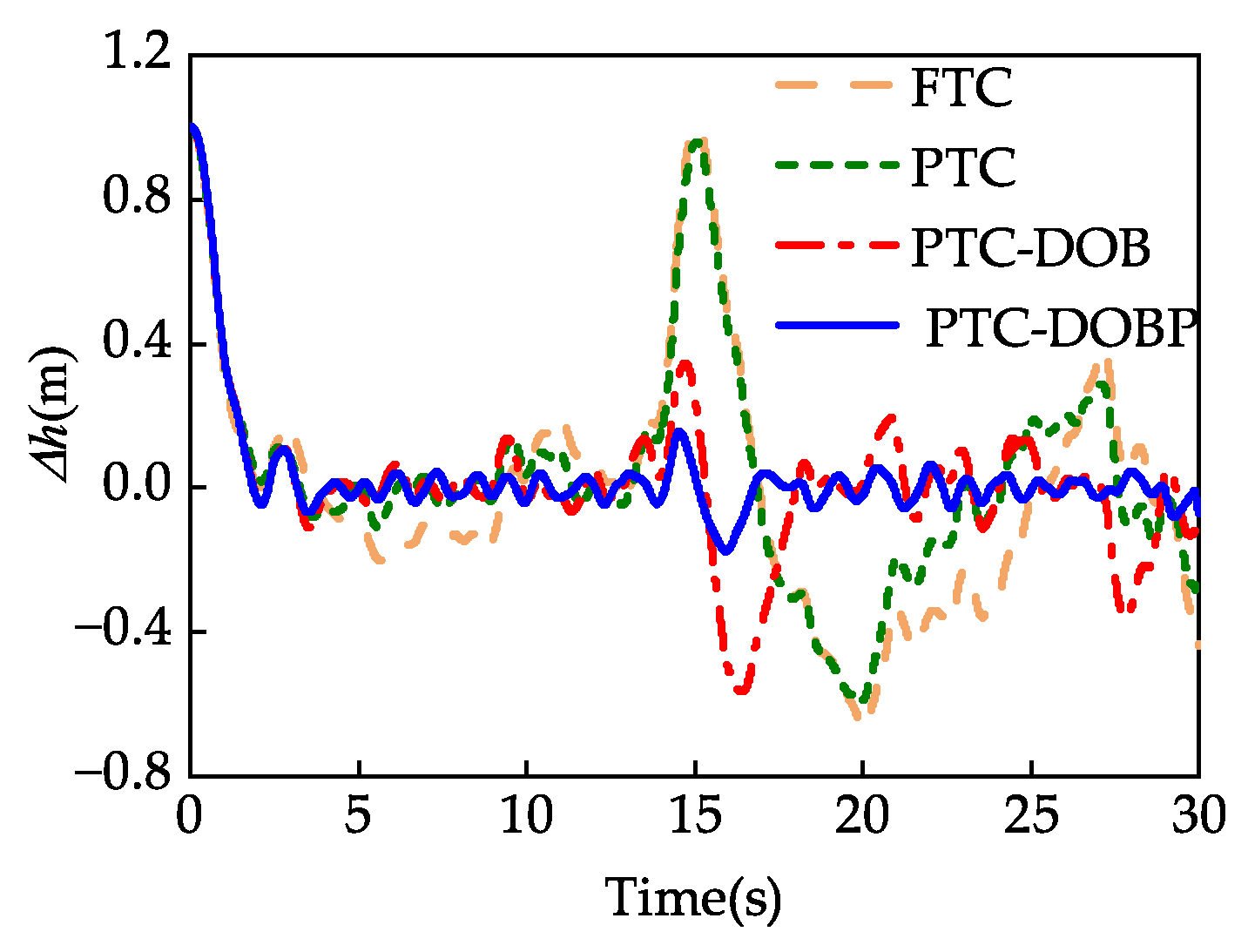
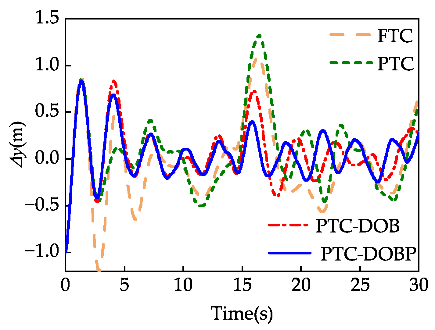
Figure 8 and Figure 9 present the longitudinal landing path and the altitude errors under four methods. Although all three methods can guide the UAV to follow the longitudinal reference path, their following error differs significantly under composite wind disturbances. During the initial landing phase, all controllers drive the altitude error to within a small neighborhood of zero within the predefined time. In about 15 s, the UAV is subjected to severe gust disturbances. For the FTC and PTC methods, PTC exhibits better initial convergence performance than FTC. However, the gust disturbances still lead to pronounced altitude errors, revealing their weakness in suppressing transient disturbances. By contrast, PTC-DOB achieves obviously improved altitude regulation by estimating and compensating for external disturbances. With further integration of the disturbance prediction module, PTC-DOBP reduces altitude error further, indicating that predictive information enables anticipatory compensation and thereby suppresses gust-induced errors. In the final phase, the airwake effect becomes sharp as the UAV approaches the carrier stern. The results show that PTC-DOBP produces the smallest altitude error among the four methods. Overall, compared with pure feedback control or observer-based compensation, the integrated observation and prediction mechanism provides more active anti-disturbance performance, thereby improving longitudinal following accuracy and improving safety margins during carrier landing.
To quantitatively evaluate the longitudinal performance of the three methods, four evaluation metrics are adopted: the maximum error after the predefined time (ME), the integral of absolute error (IAE, 0 T e t d t ), the integral of time absolute error (ITAE, 0 T t e t d t ), and the longitudinal position error (PE) between the touchdown point and DTP. The corresponding statistical results are summarized in Table 1.
As shown in Figure 9 and Table 1, PTC-DOBP exhibits the best longitudinal performance among the four methods. Compared to FTC, PTC, and PTC-DOB, the ME of PTC-DOBP is reduced by 82.0%, 81.3%, and 68.4%, indicating the large safety margin. Moreover, the IAE and ITAE decrease by 48.5–87.4% compared with those of FTC, PTC, and PTC-DOB, confirming lower accumulated following errors and enhanced longitudinal anti-disturbance performance. As for longitudinal PE, PTC-DOBP achieves reductions of 84.1%, 79.2%, and 56.5% relative to FTC, PTC, and PTC-DOB, demonstrating greater alignment with the DTP and contributing to reliable engagement of the arresting cables. Overall, the observation–prediction–compensation framework enables PTC-DOBP to outperform other methods in terms of longitudinal path following performance under composite wind disturbances.
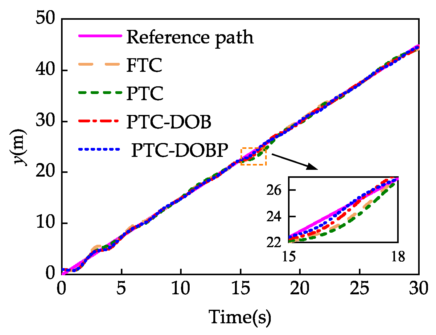
Figure 10 and Figure 11 illustrate the lateral landing path and lateral errors under four control methods. It can be seen that all methods enable the UAV to follow the lateral reference path. Nevertheless, their anti-disturbance capabilities differ markedly under wind disturbances. During the initial phase, the FPT algorithm exhibited significant overshoot. In contrast, the initial lateral error under PTC, PTC-DOB, and PTC-DOBP converged within the predefined time, indicating satisfactory transient performance. In about 15 s, however, severe lateral gusts induce large following errors under PTC and FTC, revealing their limited ability to suppress lateral gust disturbances. By incorporating a disturbance observer, PTC-DOB significantly reduces the lateral following error, thereby demonstrating the effectiveness of disturbance estimation and compensation. Furthermore, with the addition of disturbance prediction, PTC-DOBP achieves the smallest lateral error among the four methods. This result suggests that combining disturbance estimation and prediction enables more effective active compensation of gust disturbances, thereby improving lateral landing accuracy.
Compared with the longitudinal channel, the lateral channel exhibits relatively larger following errors. This can be attributed to the DLC in the longitudinal control, which provides rapid altitude regulation and enhances vertical disturbance rejection. To further quantify the lateral control performance, Table 2 summarizes the evaluation metrics for the three methods in the lateral channel.
As shown in Figure 11 and Table 2, PTC-DOBP outperforms other methods in terms of overall lateral performance. Specifically, compared with FTC, PTC, and PTC-DOB, the maximum lateral following error is reduced by 39.5%, 47.8%, and 16.9%, indicating that PTC-DOBP increases the safety margin. In addition, the IAE and ITAE of PTC-DOBP decrease by 15.6–54.5% relative to FTC, PTC, and PTC-DOB, confirming lower accumulated following errors and improved anti-disturbance capability. As for lateral PE, PTC-DOBP performs comparably to PTC-DOB and achieves reductions of 59.7% and 53.4% relative to FPT and PTC, respectively. This improvement enhances the UAV to align accurately with the center of the arresting cables, thereby reducing the risk of lateral skidding on the carrier deck. Overall, through feedforward compensation that integrates disturbance observation and prediction, PTC-DOBP significantly reduces lateral path following error under composite wind disturbances.
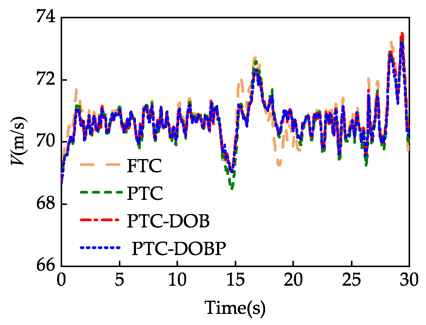
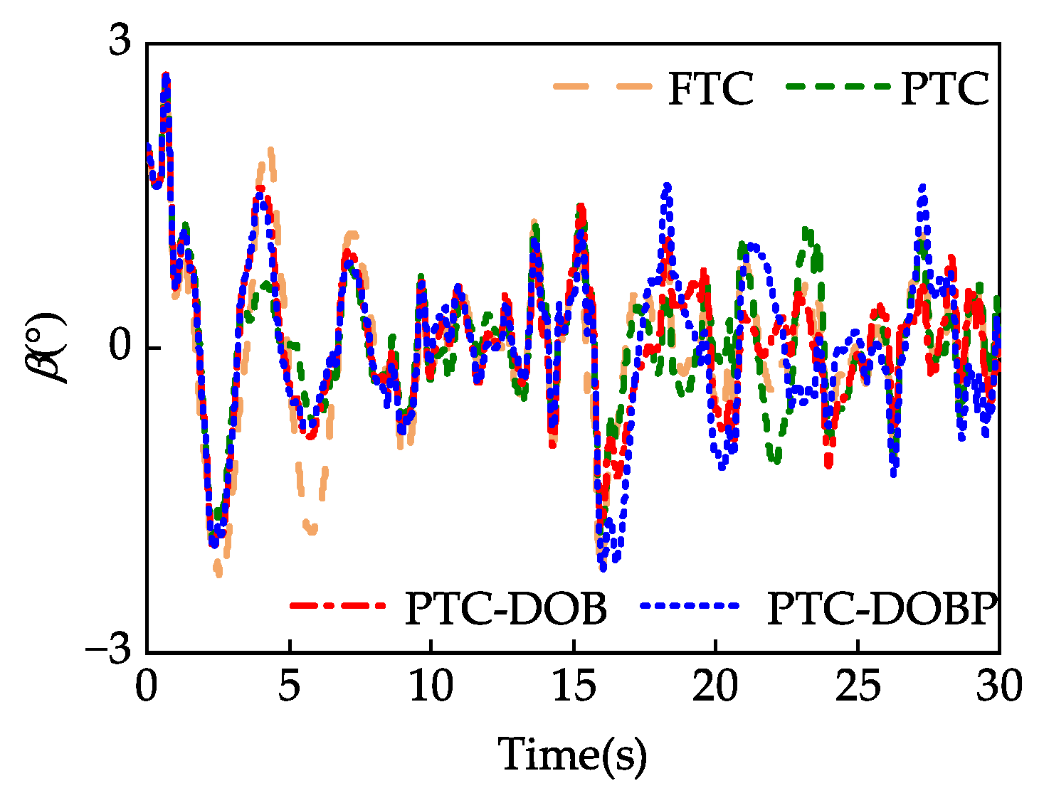
Figure 12, Figure 13 and Figure 14 present the responses of the UAV’s velocity, AOA, and sideslip angle under the four control methods. It can be seen that all controllers maintain these states stable, thereby ensuring flight stability during carrier landing under low dynamic pressure conditions. During the initial phase, errors in velocity, AOA, and sideslip angle rapidly converged under all four controllers, indicating satisfactory transient response. In about 15 s, severe gust disturbances induce pronounced oscillatory responses. Specifically, the longitudinal, vertical, and lateral gusts affect the velocity, AOA, and sideslip angle, respectively, resulting in transient triangular-like fluctuations with different amplitudes. The state responses under all controllers exhibit similar trends and gradually return to steady conditions, demonstrating effective anti-gust performance. In the terminal phase, strong longitudinal and vertical airwake components lead to larger fluctuations in velocity and AOA. Since the lateral airwake component is relatively weak, the sideslip angle error remains with small fluctuations. Furthermore, the more aggressive altitude error regulation in the proposed PTC-DOBP method leads to slightly larger oscillations in the AOA. However, these oscillations remain within safe limits and are accompanied by improved path following performance.
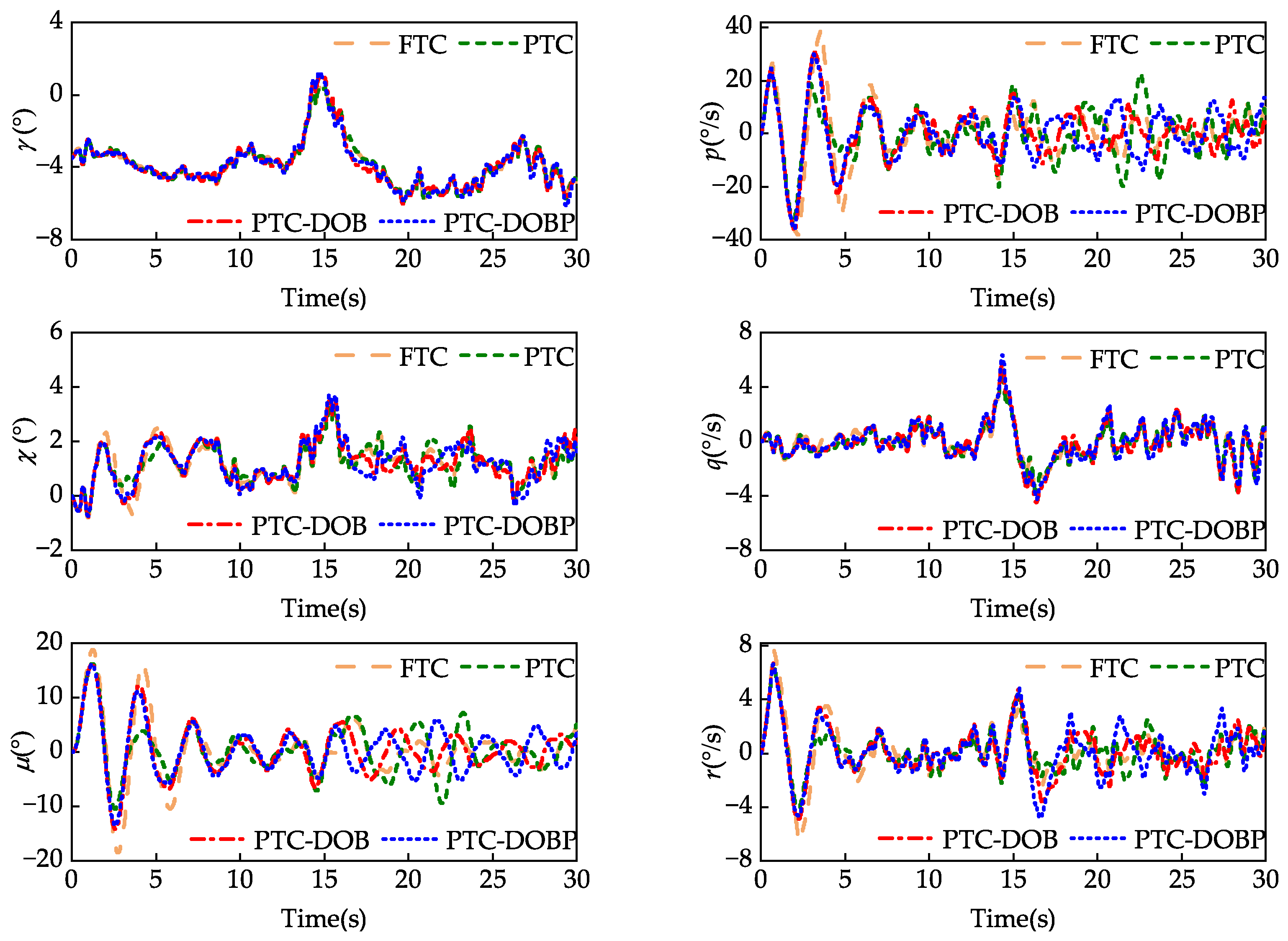
Figure 15 illustrates the responses of the UAV’s COA, heading angle, roll angle, and body-axis angular rates during carrier landing. It can be seen that these variables exhibit similar dynamic characteristics under the four control methods. The COA remains around −3.5°, while pronounced triangular-like oscillations appear around 15 s owing to gust disturbances. In the terminal landing phase, the oscillation amplitude increases under severe airwake effects. Consistent with this behavior, the pitch rate shows a similar trend, providing the angular rate support for the rapid longitudinal attitude correction and AOA stabilization. The heading and roll angles undergo rapid initial adjustments, thereby effectively reducing the lateral position and attitude errors. Subsequently, both variables gradually converge, with the heading angle stabilizing at approximately 1° and the roll angle at 0°. Since the carrier speed is constant and a slight angle exists between the angled deck and the carrier heading, the DTP maintains a constant lateral velocity. Therefore, a nonzero heading angle is required to achieve accurate following of the lateral landing path. The yaw and roll rates also exhibit similar response trends. The sharp initial transients provide the angular rate commands required for lateral position and attitude correction. Moreover, the sawtooth-like oscillations around 15 s indicate compensatory control actions generated by the controllers in response to wind disturbances, which maintain lateral attitude and position stability.
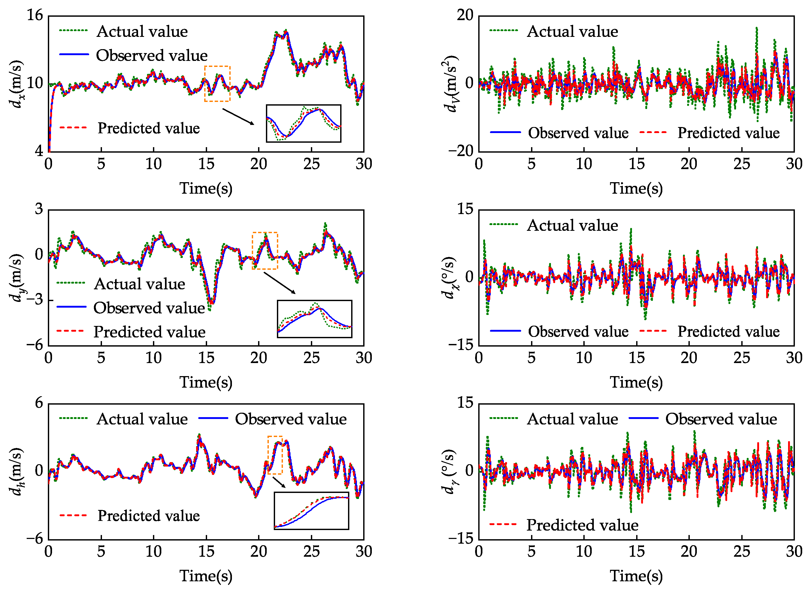
Figure 16 illustrates the actual disturbance, the observed disturbance, and the predicted disturbance. The results show that the proposed PTDOB rapidly and accurately estimates the external disturbance caused by composite wind. The observation error converges to a small neighborhood of the origin within the predefined time, demonstrating excellent rapidity and convergence performance. However, the PTDOB output exhibits a dynamic lag relative to the actual disturbance. To address this issue, the proposed disturbance predictor based on the FFRLS predicts disturbance online. By taking the weighted average of the predicted values over 10 prediction steps, the final disturbance compensation signal improves prediction accuracy and robustness. The enlarged views indicate that the compensation signal provides a lead margin, effectively compensating for the observation lag and enabling the UAV to suppress external disturbances more promptly. Consequently, disturbance observation is primarily used to accurately estimate the current disturbance, while disturbance prediction is introduced to compensate for the degraded transient control performance caused by the PTDOB output lag. By providing a compensation signal with a certain lead margin, the predictor alleviates observer lag and system response delay. Consequently, integrating observation and prediction achieves more effective active anti-disturbance performance than either method alone.

6. Conclusions

This paper investigates the design of ACLS with predefined-time convergence, accurate path following, and effective anti-disturbance in the presence of complex wind disturbances. An active anti-disturbance control method is developed by combining predefined-time sliding mode control, disturbance observation, and online disturbance prediction. The simulation results indicate that the proposed method ensures the convergence of flight state errors within a user-specified time under different initial error conditions, thus improving the dynamic response. In the comparative experiment under complex wind conditions, the PTDOBP provides accurate estimation and prediction of disturbances caused by steady wind, gusts, and airwake, effectively compensating for the observer lag. Compared with FTC, PTC, and PTC-DOB, the proposed PTC-DOBP method reduces the maximum altitude error and lateral error by 16.9–82.0%, and reduces the landing point error by about 53.4–84.1%. These results suggest that PTC-DOBP enhances ACLS’s active anti-disturbance capability and improves DSP following performance during carrier landing under complex wind environments. Future work will focus on the performance limits of the proposed method under stronger disturbances and more extreme turbulent environments, as well as a dedicated robust design for unmodeled dynamics and parameter uncertainties. In addition, further studies will consider non-ideal sensing conditions such as sensor noise and measurement delays, implementation on a scaled-down UAV, and the extension of the proposed framework to more complex scenarios, including multi-UAV cooperative landing.

Author Contributions

Conceptualization, Q.Z. and Z.W.; methodology, Q.Z. and Z.W.; software, Z.W.; validation, Z.W.; formal analysis, Z.W. and W.J.; investigation, Z.W. and P.S.; resources, Q.Z., W.J. and L.W.; data curation, Z.W., P.S. and W.J.; writing—original draft preparation, Z.W. and P.S.; visualization, Z.W. and P.S.; supervision, Q.Z., W.J. and L.W.; project administration, Q.Z., and L.W.; funding acquisition, Q.Z. and L.W.; All authors have read and agreed to the published version of the manuscript.

Funding

This research was funded by the National Natural Science Foundation of China (No. 52171299 and 62573151), the Natural Science Foundation of Heilongjiang Province of China (No. LH2024F037), and the Fundamental Research Funds for the Central Universities of China (No. 3072024XX0403).

Data Availability Statement

The data that support the findings of this study are available on request from the corresponding author, upon reasonable request, and with the permission of the laboratory confidentiality agency.

Conflicts of Interest

The authors declare no conflicts of interest. Author Mr. Wenqiang Jiang was employed by the company China Ship Development and Design Center, Wuhan, China. The remaining authors declare that the research was conducted in the absence of any commercial or financial relationships that could be construed as a potential conflict of interest.

Appendix A

I 1 = I y I z I z 2 I x z 2 I s u m , I 2 = I x I y + I z I x z I s u m , I 3 = I z I s u m , I 4 = I x z I s u m , I 5 = I z I x I y
I 6 = I x z I y , I 7 = 1 I y , I 8 = I x 2 I x I y + I x z 2 I s u m , I 9 = I x I s u m , I s u m = I x I z I x z 2
d 1 = d x d y d h T = u v w T
d χ = 1 V a u ˙ sin χ v ˙ cos χ
d V = u ˙ cos χ cos γ v ˙ sin χ cos γ + w ˙ sin γ
d 4 = d γ 0 0 0 T = 1 V a u ˙ cos χ sin γ + v ˙ sin χ sin γ + w ˙ cos γ 0 0 0 T
g 1 = V a 0 0 V a
f χ = sin μ m V a cos γ L + T sin α μ + cos μ m V a cos γ Y T cos α sin β
g χ = sin μ m V a cos γ
f 3 = sec β γ ˙ cos μ + χ ˙ sin μ cos γ γ ˙ sin μ + χ ˙ cos μ cos γ γ ˙ tan β cos μ + χ ˙ sin γ + tan β sin μ cos γ
g 3 = cos α tan β 1 sin α tan β sin α 0 cos α sec β cos α 0 sec β sin α
f 4 = cos μ m V a q ¯ s ( C L 0 + C L α α ) + T sin α sin μ m V a Y T cos α sin β g V a cos γ I 1 q r + I 2 q p + I 3 q ¯ s b L b + I 4 q ¯ s b N b I 5 p r + I 6 r 2 I 6 p 2 + I 7 q ¯ s c ¯ C m 0 + C m α α + C m q q c ¯ 2 V a I 8 p q I 2 q r + I 4 q ¯ s b L b + I 9 q ¯ s b N b
L b = C L ¯ β β + C L ¯ p p b ¯ 2 V a + C L ¯ r r b ¯ 2 V a , N b = C n β β + C n p p b ¯ 2 V a + C n r r b ¯ 2 V a .
g 4 = cos μ m V a q ¯ s C L δ f 0 cos μ m V a q ¯ s C L δ e 0 0 q ¯ s b I 3 C L ¯ δ a + I 4 C n δ a 0 q ¯ s b I 3 C L ¯ δ r + I 4 C n δ r q ¯ s c ¯ I 7 C m δ f 0 q ¯ s c ¯ I 7 C m δ e 0 0 q ¯ s b I 4 C L ¯ δ a + I 9 C n δ a 0 q ¯ s b I 4 C L ¯ δ r + I 9 C n δ r
f V = Y sin β m D m g sin γ
g V = T max cos α cos β m
Table A1. Initial conditions of UAV and aircraft-based carrier.
StateValueStateValue
[ x 0 , y 0 , h 0 ] (m) [ 0 , 1 , 147 ] [ x c 0 , y c 0 , z c 0 ] (m) [ 2056.2 , 0 , 0 ]
[ γ 0 , χ 0 ] ( ° ) [ 3.5 , 0 ] [ p 0 , q 0 , r 0 ] (°/s) [ 0 , 0 , 0 ]
[ α 0 , β 0 , μ 0 ] ( ° ) [ 10.1 , 2 , 0 ] [ V 0 , V c ] ( m / s ) [ 68 , 10 ]
Table A2. The model parameters of actuators.
ActuatorsLimit (°)Rate (°/s)Model
Flap( 15 , 25 )( 40 , 40 ) 30 30 s + 30 s + 30
Elevator( 20 , 20 )( 100 , 100 ) 48 48 s + 48 s + 48
Aileron( 20 , 20 )( 40 , 40 ) 30 30 s + 30 s + 30
Rudder( 20 , 20 )( 40 , 40 ) 40 40 s + 40 s + 40
Table A3. List of acronyms used in this paper.
AcronymDefinitionAcronymDefinition
ACLS Automatic carrier landing system UAV Unmanned aerial vehicle
DSP Desired slope path DTP Desired touchdown point
6 - DOF Six degrees of freedom AOA Angle of attack
COA Climb angle APCS Approach power compensation system
DLC Direct lift control SMC Sliding mode control
FTC Fixed-time control PTC Predefined-time control
PTS Predefined-time stability PTRM Predefined-time reference model
PTSMC Predefined-time sliding mode control PTDOB Predefined-time disturbance observer
PTDOBP Predefined-time disturbance observer and predictor ESO Extended state observer
AR Autoregressive FFRLS Recursive least squares with forgetting factor
PTC - DOB Predefined-time control with disturbance observer PTC - DOBP Predefined-time control with disturbance observer and prediction
ME Maximum error PE Position error
IAE Integral of absolute error ITAE Integral of time absolute error

References

  1. Jia, B.; Sun, L.; Liu, X.; Xu, S.; Tan, W.; Jiao, J. Carrier aircraft flight controller design by synthesizing preview and nonlinear control laws. Drones 2023, 7, 200. [Google Scholar] [CrossRef]
  2. Duan, H.; Chen, L.; Zeng, Z. Automatic landing for carrier-based aircraft under the conditions of deck motion and carrier airwake disturbances. IEEE Trans. Aerosp. Electron. Syst. 2022, 58, 5276–5291. [Google Scholar] [CrossRef]
  3. Chen, H.A.; Wen, Z.Y.; Zhang, Y.; Su, G.Q.; Wu, L.N.; Xie, K. Wind-resistant UAV landing control based on drift angle control strategy. Aerospace 2025, 12, 678. [Google Scholar] [CrossRef]
  4. Citroni, R.; Di Paolo, F.; Livreri, P. A novel energy harvester for powering small UAVs: Performance analysis, model validation and flight results. Sensors 2019, 19, 1771. [Google Scholar] [CrossRef]
  5. Sun, N.; Duan, H.; Huo, M. Automatic carrier landing control of carrier-based UAV under actuator failure condition. Aerosp. Sci. Technol. 2025, 160, 110067. [Google Scholar] [CrossRef]
  6. Fu, M.; Wang, L. Finite-time path following control of an underactuated marine surface vessel with input and output constraints. Appl. Sci. 2020, 10, 6447. [Google Scholar] [CrossRef]
  7. Zhang, S.; Nan, Y.; Li, Z. Moving path following with adaptive neural network finite-time recursive sliding mode control for carrier landing with uncertain dynamics and saturation. Aerosp. Sci. Technol. 2024, 150, 109220. [Google Scholar] [CrossRef]
  8. Liu, Z.; Zhang, O.; Gao, Y.; Zhao, Y.; Sun, Y.; Liu, J. Adaptive neural network-based fixed-time control for trajectory tracking of robotic systems. IEEE Trans. Circuits Syst. II Express Briefs 2022, 70, 241–245. [Google Scholar] [CrossRef]
  9. Kumar, S.; Sinha, A.; Kumar, S.R. Robust path-following guidance for an autonomous vehicle in the presence of wind. Aerosp. Sci. Technol. 2024, 150, 109225. [Google Scholar] [CrossRef]
  10. Guan, Z.; Liu, H.; Zheng, Z.; Lungu, M.; Ma, Y. Fixed-time control for automatic carrier landing with disturbance. Aerosp. Sci. Technol. 2021, 108, 106403. [Google Scholar] [CrossRef]
  11. Nguyen, V.C.; Kim, S.H. A novel fixed-time prescribed performance sliding mode control for uncertain wheeled mobile robots. Sci. Rep. 2025, 15, 5340. [Google Scholar] [CrossRef]
  12. Li, Y.; Liu, X.; Zhen, Z.; Wen, C.Y.; Zheng, Y. Direct lift control for carrier-based aircraft with predefined-time incremental strategy. IEEE Trans. Aerosp. Electron. Syst. 2025, 61, 11528–11542. [Google Scholar] [CrossRef]
  13. Yao, Z.; Kan, Z.; Li, D.; Shao, H.; Xiang, J. Global fast terminal sliding mode control for automatic carrier landing with environmental disturbances. Aircr. Eng. Aerosp. Technol. 2024, 96, 465–474. [Google Scholar] [CrossRef]
  14. Vilcica, D.; Lungu, M.; Chen, M.; Tudosie, A. Four-stage cascaded adaptive sliding mode control for automatic carrier landing with airwake disturbances and uncertainties. Appl. Math. Model. 2025, 138, 115729. [Google Scholar] [CrossRef]
  15. Yao, Z.; Li, D.; Kan, Z. Adaptive terminal sliding combined super twisting control design and flight tests for automatic carrier landing system. Chin. J. Aeronaut. 2025, 38, 103202. [Google Scholar] [CrossRef]
  16. Yu, Y.; Chen, J.; Zheng, Z.; Yuan, J. Distributed finite-time ESO-based consensus control for multiple fixed-wing UAVs subjected to external disturbances. Drones 2024, 8, 260. [Google Scholar] [CrossRef]
  17. Yuan, Y.; Duan, H.; Zeng, Z. Automatic carrier landing control with external disturbance and input constraint. IEEE Trans. Aerosp. Electron. Syst. 2022, 59, 1426–1438. [Google Scholar] [CrossRef]
  18. Yao, Z.; Kan, Z.; Li, D.; Shao, H.; Jiang, Y.; Xiang, J. Active anti-disturbance carrier landing control with integrated direct lift. Comput. Electr. Eng. 2024, 120, 109699. [Google Scholar] [CrossRef]
  19. Wu, Q.; Zhu, Q. Fault-tolerant control of automatic carrier landing using direct lift control based on nonsingular terminal sliding mode and active disturbance rejection control. Trans. Inst. Meas. Control 2025, 47, 29–40. [Google Scholar] [CrossRef]
  20. Zhen, Z.; Jiang, S.; Ma, K. Automatic carrier landing control for unmanned aerial vehicles based on preview control and particle filtering. Aerosp. Sci. Technol. 2018, 81, 99–107. [Google Scholar] [CrossRef]
  21. Meng, Y.; Wang, W.; Han, H. Flight control method using neural network in prediction for suppressing ship airwake impact in carrier landing. IEEE Aerosp. Electron. Syst. Mag. 2023, 38, 20–32. [Google Scholar] [CrossRef]
  22. Wang, L.; Zhang, Z.; Zhu, Q.; Wen, Z. Longitudinal automatic carrier-landing control law rejecting disturbances and coupling based on adaptive dynamic inversion. Bull. Pol. Acad. Sci. Tech. Sci. 2021, 69, e136217. [Google Scholar] [CrossRef]
  23. Duan, H.; Yuan, Y.; Zeng, Z. Automatic carrier landing system with fixed time control. IEEE Trans. Aerosp. Electron. Syst. 2022, 58, 3586–3600. [Google Scholar] [CrossRef]
  24. Guan, Z.; Ma, Y.; Zheng, Z.; Guo, N. Prescribed performance control for automatic carrier landing with disturbance. Nonlinear Dyn. 2018, 94, 1335–1349. [Google Scholar] [CrossRef]
  25. Beard, R.; Ferrin, J.; Humpherys, J. Fixed wing UAV path following in wind with input constraints. IEEE Trans. Control. Syst. Technol. 2014, 22, 2103–2117. [Google Scholar] [CrossRef]
  26. United States Department of Defense. MIL-F-8785C. In Flying Qualities of Piloted Airplanes, Revision C Nov.; United States Department of Defense: Washington, DC, USA, 1980. [Google Scholar]
  27. Lungu, M.; Dinu, D.; Chen, M.; Flores, G. Inverse optimal control for autonomous carrier landing with disturbances. Aerosp. Sci. Technol. 2023, 139, 108382. [Google Scholar] [CrossRef]
  28. Zhang, S.; Qiu, Y.; Sun, J.; Wang, B.; Gao, Z. Gust load alleviation control strategies for large civil aircraft through wing camber technology. Actuator 2024, 13, 229. [Google Scholar] [CrossRef]
  29. Zhang, M.; Zang, H.; Bai, L. A new predefined-time sliding mode control scheme for synchronizing chaotic systems. Chaos Solitons Fractals 2022, 164, 112745. [Google Scholar] [CrossRef]
  30. Xie, S.; Chen, Q. Predefined-time disturbance estimation and attitude control for rigid spacecraft. IEEE Trans. Circuits Syst. II Express Briefs 2023, 71, 2089–2093. [Google Scholar] [CrossRef]
  31. Polycarpou, M.M.; Weaver, S.E. Stable adaptive neural control of nonlinear systems. In Proceedings of the American Control Conference, Seattle, WA, USA, 21–23 June 1995; pp. 847–851. [Google Scholar]
  32. Xie, S.; Chen, Q.; Yang, Q. Adaptive fuzzy predefined-time dynamic surface control for attitude tracking of spacecraft with state constraints. IEEE Trans. Fuzzy Syst. 2022, 31, 2292–2304. [Google Scholar] [CrossRef]
  33. Liu, Z.; Bechlioulis, C.P.; Huang, J.; Wen, C. Nonlinear dynamic surface control for a class of uncertain systems with novel nonlinear filters. IEEE Trans. Autom. Control 2025, 70, 8290–8297. [Google Scholar] [CrossRef]
  34. Chen, J.; Chen, Z.; Zhang, H.; Xiao, B.; Cao, L. Predefined-time observer-based nonsingular sliding-mode control for spacecraft attitude stabilization. IEEE Trans. Circuits Syst. II Express Briefs 2023, 71, 1291–1295. [Google Scholar] [CrossRef]
  35. Wang, Z.; Zhu, Q.; Zhao, T.; Wang, L. An optimal guidance law based on deep reinforcement learning for compensating the lag in time-varying slope path following. Aerosp. Sci. Technol. 2026, 168, 110948. [Google Scholar] [CrossRef]
  36. Chen, Y.; Huang, Y.; Song, Z. Vehicle state estimation by integrating the recursive least squares method with a variable forgetting factor with an adaptive iterative extended kalman filter. World Electr. Veh. J. 2024, 15, 399. [Google Scholar] [CrossRef]
  37. Tan, M.; Xiang, G.; Xiang, X.; Yu, S.; Rao, K.; Soares, C. Directional and adaptive forgetting factor based recursive least square algorithms for maneuvering dynamic identification and motion prediction of unmanned surface vessel. Ocean Eng. 2025, 342, 122948. [Google Scholar] [CrossRef]
  38. Steinert, A.; Raab, S.; Hafner, S.; Holzapfel, F.; Hong, H.C. From fundamentals to applications of incremental nonlinear dynamic inversion: A survey on INDI - Part I. Chin. J. Aeronaut. 2025, 38, 103553. [Google Scholar] [CrossRef]
  39. Lungu, M.; Chen, M.; Ebrahimpour, M.; Guo, H. Dynamic inversion- and neural network-based five-stage cascaded control for automatic carrier landing subject to multiple disturbances and uncertainties. J. Frankl. Inst. 2025, 362, 107719. [Google Scholar] [CrossRef]
  40. Varriale, C.; Lombaerts, T.; Looye, G. Direct lift control: A review of its principles, merits, current and future implementations. Prog. Aerosp. Sci. 2025, 152, 101073. [Google Scholar] [CrossRef]
  41. Peng, X.; Li, Y.; Wang, Z. Observer-enhanced sliding mode control for fixed-wing aircraft automatic carrier landing. ISA Trans. 2025, 167, 1431–1445. [Google Scholar] [CrossRef]
Figure 1. The schematic of the carrier landing under complex wind disturbances.
Drones 10 00308 g001
Figure 2. The framework of the ACLS.
Drones 10 00308 g002
Figure 3. Altitude error responses under different initial errors.
Drones 10 00308 g003
Figure 4. Lateral position error responses under different initial errors.
Drones 10 00308 g004
Figure 5. Velocity error responses under different initial errors.
Drones 10 00308 g005
Figure 6. AOA error responses under different initial errors.
Drones 10 00308 g006
Figure 7. Sideslip angle error responses under different initial errors.
Drones 10 00308 g007
Figure 8. Longitudinal landing paths under different methods.
Drones 10 00308 g008
Figure 9. Altitude errors under different methods.
Drones 10 00308 g009
Figure 10. Lateral landing paths under different methods.
Drones 10 00308 g010
Figure 11. Lateral errors under different methods.
Drones 10 00308 g011
Figure 12. Velocity errors under different methods.
Drones 10 00308 g012
Figure 13. AOA errors under different methods.
Drones 10 00308 g013
Figure 14. Sideslip angle errors under different methods.
Drones 10 00308 g014
Figure 15. Different flight state responses under different methods.
Drones 10 00308 g015
Figure 16. The comparison between the actual, observed, and predicted disturbances.
Drones 10 00308 g016
Table 1. Longitudinal evaluation metrics of FTC, PTC, PTC-DOB, and PTC-DOBP.
MethodMEIAEITAEPE
FTC1.007.41115.787.14
PTC0.965.9892.365.44
PTC-DOB0.573.5748.152.60
PTC-DOBP0.181.8414.641.13
Table 2. Lateral evaluation metrics of PTC, PTC-DOB, and PTC-DOBP.
MethodMEIAEITAEPE
FTC1.1410.29138.280.67
PTC1.329.13135.070.58
PTC-DOB0.836.5277.830.29
PTC-DOBP0.695.5062.900.27
Disclaimer/Publisher’s Note: The statements, opinions and data contained in all publications are solely those of the individual author(s) and contributor(s) and not of MDPI and/or the editor(s). MDPI and/or the editor(s) disclaim responsibility for any injury to people or property resulting from any ideas, methods, instructions or products referred to in the content.