


Highlights
What are the main findings?
- A new HTMRG construction method is introduced based on grid maps. Through skeleton simplification, redundant hub-node merging, intersection-region modeling, and the generation of smooth corridor (SCE) and intersection edges (SIE), it produces a structurally compact, globally navigable, and geometrically continuous road network.
- A visibility-based start–goal insertion strategy significantly shortens planned path length in simulations, Gazebo tests, and real-world experiments, improving overall path-planning efficiency.
What are the implications of the main findings?
- HTMRG enables fast computation of geometrically continuous and directly trackable paths, achieving improved smoothness and execution stability compared with GVD, HTG, and grid-based methods.
- The framework demonstrates robust performance across structured and unstructured environments and is validated through simulations and real-world tests, supporting reliable deployment in practical UGV navigation tasks.
Abstract
Autonomous navigation in complex environments requires efficient and reliable road-network representations for fast path planning. However, traditional grid and skeleton-based approaches often suffer from high computational cost and limited path quality. This paper proposes a Hierarchical Topology-Metric Road Graph (HTMRG) framework for autonomous navigation of unmanned ground vehicles (UGVs). The method automatically constructs a hierarchical road graph from grid maps by identifying key intersection structures and generating smooth corridor and intersection connections. In addition, a dedicated start–goal insertion strategy is developed to enable efficient graph-based path planning in previously unexplored scenarios. Extensive simulations and real-world experiments demonstrate that the proposed method can automatically construct hierarchical road graphs and generate smooth, high-quality paths with improved planning efficiency and robustness. The HTMRG framework has also been successfully integrated into a UGV system, validating its effectiveness and practicality in real-world navigation scenarios.
1. Introduction
Autonomous navigation in complex and large-scale environments is a fundamental capability for unmanned ground vehicles (UGVs) in applications such as Automated Guided Vehicle (AGV) transportation [1], contactless delivery [2], and self-driving [3]. Efficient global path planning relies heavily on compact and informative representations of the robot’s free space, which must balance computational efficiency, path quality, and safety.
Road Graphs (RGs) provide a promising representation by abstracting the navigable free space into a graph structure that supports fast search and decision-making. However, constructing RGs that simultaneously ensure computational efficiency, geometric accuracy, and path smoothness remains a challenging problem, especially in environments that contain both structured and unstructured regions. In autonomous robotics, Global Path Planning (GPP) is often required as an essential input for motion planning and control. Despite its importance, existing RG modeling approaches still struggle to balance graph compactness, planning efficiency, and trajectory smoothness across diverse environments.
A wide range of navigation map modeling methods have been explored in the literature. The current mainstream navigation map modeling methods include grid maps, geometric maps, topology maps, route maps, etc. The grid map is the most common type of map representation, but its accuracy is limited by cell resolution [4]. Geometric maps are used to describe the free space of the environment using shapes and coordinates, providing detailed spatial information [5]. Paths can be planned using spatial sampling, numerical optimization methods, or more recently learning-based and data-driven [6] planning approaches. However, sampling-based GPP methods are influenced by the sampling step size [7], while numerical optimization methods are computationally complex and prone to getting stuck in local optimum.
The Visibility Graph (VG) method assumes that the robot is represented as a point and obstacles are approximated as polygons [8]. It connects the start point, goal point, and vertices of polygons with visible line segments. These line segments cannot intersect with the polygons of obstacles [9]. Path planning is then based on the visibility graph formed by these points and edges. The resulting path tends to be tortuous and uneven, as it follows line segments connecting the vertices of obstacles. This makes it prone to collisions with obstacles and lacking in flexibility, thus making it challenging to use directly for path guidance. Therefore, smoothing techniques are required to refine the trajectory in subsequent applications [10]. Additionally, an increased number of environmental obstacles and richer feature information lead to longer search times.
The Probability Roadmap (PRM) method creates an undirected graph by sampling and performing collision detection to determine the connectivity between sampling points in free space. Feasible paths can then be obtained through graph search. A disadvantage of this algorithm is its limited suitability for complex environments and low completeness. Specifically, if the parameters are set incorrectly, even existing feasible paths may not be discovered. Moreover, the planned paths tend to be uneven and are difficult to use directly for tracking and guidance [11].
High-definition maps, such as Lanelet2, OpenDRIVE, and Apollo [12] are widely used in self-driving applications. Silva [13] utilized Clothoids to construct sparse road network models for autonomous navigation. Mi [14] proposed a method for extracting and vectorizing 3D road boundaries from point clouds. Zhang [15] reconstructed 3D highway curves from mobile laser scanning point clouds. However, these approaches are limited to regular, structured urban highway scenarios and require substantial manual effort for further modeling.
The topology-metric RG establishes a route model with metric properties in free space to support robot path planning and navigation. Tae built a Topology Graph (TG) from the local grid map using a thinning algorithm [16]. Stenzel [17] constructed a Topology Graph (TG) for AGVs, making path finding relatively easy and fast. However, the absence of metric information results in a low accuracy of the planned route, making it unsuitable for direct application in robot tracking and guidance. In [18,19], a method based on central axis topology routes was used to improve the efficiency of PRM in constructing RGs. However, these methods are still sampling-based. The resulting roadmaps have probabilistic completeness but are not suitable for direct robot tracking. Spline-based topology generation for path planning was proposed in [20]. Although kinematic constraints were considered, validation was performed only in the structured environment simulations.
In [21,22], an explicit corridor topology map was proposed for robot navigation planning. By significantly reducing the search space, skeleton paths can be quickly obtained from the TG as needed, achieving lightweight computation. However, this approach was mainly applied to structured indoor environments, and only distinguishes between skeleton and topology points without further modeling hub intersections. Although this enhances search speed, smoothly tracking the planned path can be challenging.
This study draws inspiration from real-world structured traffic road networks to develop a method for fast, smooth, safe, and relatively short GPP, which can be used in both large-scale structured and unstructured environments for wheeled or tracked UGVs, such as Husky-class unmanned ground vehicles and similar mobile robotic platforms. The primary contributions of this study are as follows:
- Reducing the size of the TG and identifying map intersections by simplifying and merging redundant nodes.
- Constructing HTMRG by designing smooth corridor edges and intersection edges to generate navigable road routes.
- Enhancing the insertion process of start and goal nodes within the HTMRG to improve GPP performance.
- Conducting extensive simulations and real-world experiments across various environments and integrating the proposed method into UGV autonomous navigation systems.
The remainder of this paper is organized as follows. Section 2 presents the overall workflow of HTMRG. Section 3 details the construction of HTMRG. Section 4 describes its application to path planning. Section 5 reports the simulation results, while Section 6 presents the real-world experimental results. Finally, Section 7 concludes the paper and outlines future work.
2. The Workflow of HTMRG
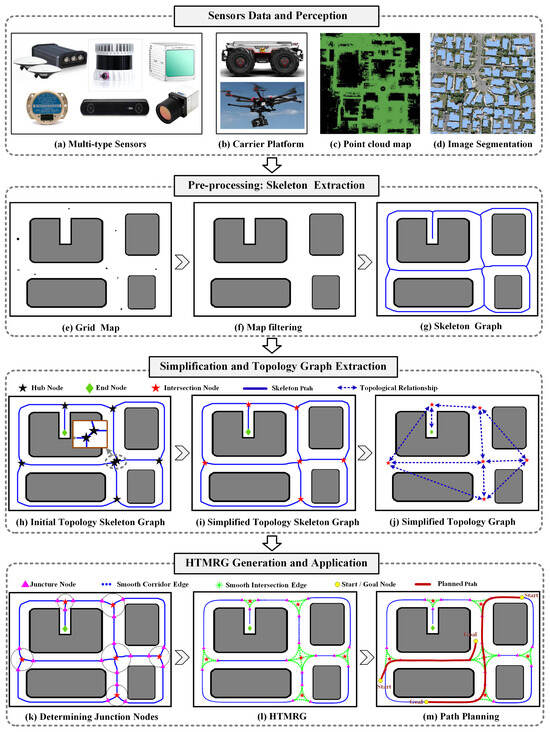
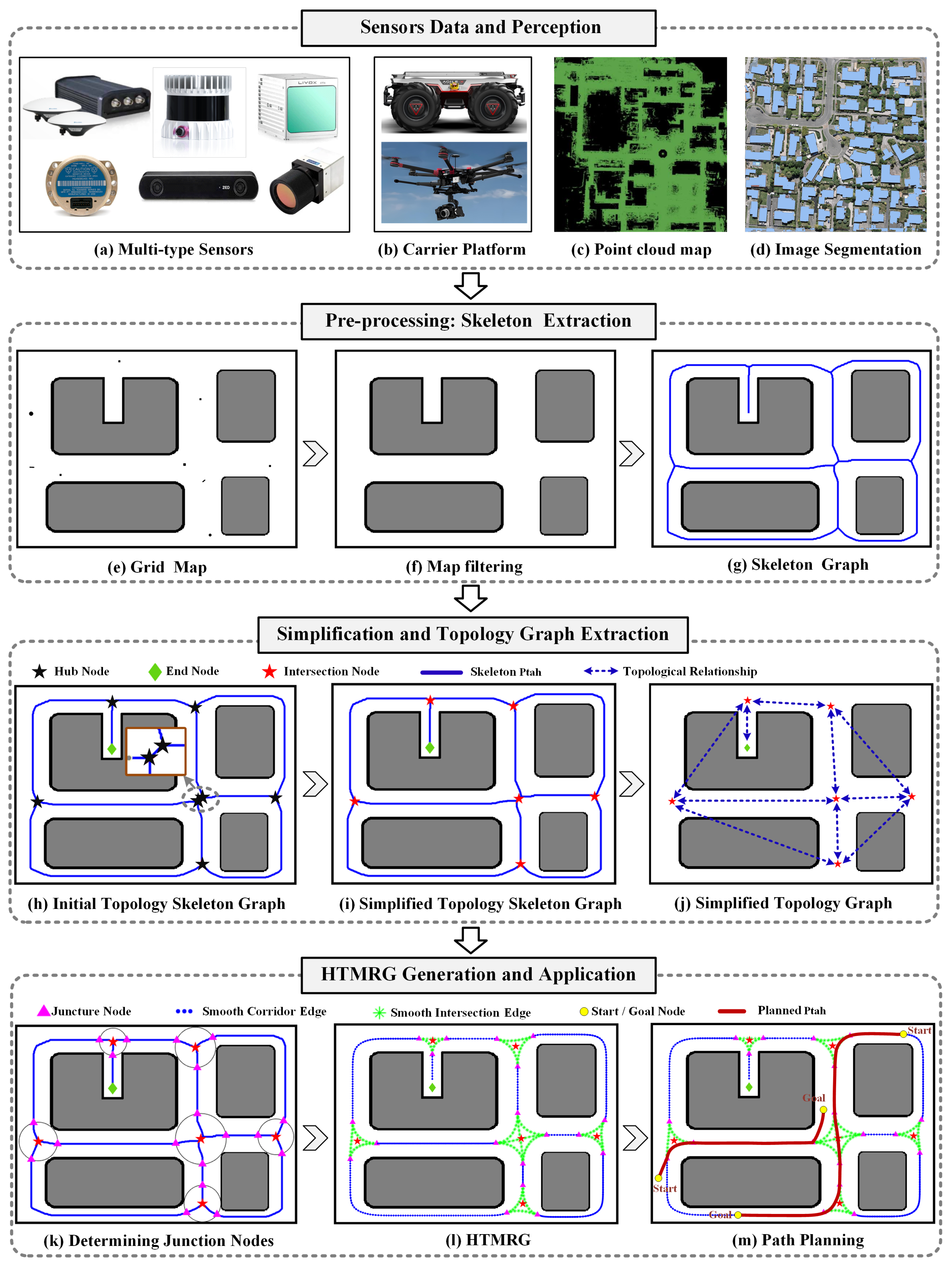
This chapter presents the workflow of the HTMRG method and defines the relevant components, laying the foundation for subsequent sections. As shown in Figure 1, the HTMRG framework can be divided into four main processes: sensors data and perception, pre-processing, simplification and TG extraction, HTMRG generation and application.
Figure 1.
Workflow of the proposed HTMRG method, including sensors data and perception, pre-processing, simplification and topology graph extraction, HTMRG generation and application.
2.1. Sensors Data and Perception
The proposed HTMRG approach takes as input a grid-based 2D map, , where I and J denote the number of rows and columns of the grid map, respectively. Each cell is binary: 0 denotes free space and 1 denotes occupancy. Unmanned carrier platforms typically perform environmental data acquisition and perception-based mapping by integrating multiple types of sensors (e.g., GPS, LiDAR, and cameras). As illustrated in Figure 1c, SLAM technology can be employed to construct global cloud maps [23], which are subsequently projected into grid maps. In addition, as shown in Figure 1d, image segmentation algorithms applied to UAV aerial imagery can be used to extract obstacles [24], thereby producing grid maps that delineate traversable areas.
2.2. Pre-Processing
In this stage, the input grid map is first filtered [25] to remove noise and then skeletonized to generate the skeleton graph (SG). The skeleton is a morphological representation of the map, positioned equidistant from the nearest obstacle points. It can be generated using various methods, such as the Voronoi diagram, image thinning, and distance field transformation [22]. Figure 1f illustrates the grid-map after filtering, while Figure 1g displays the resulting skeleton map through the distance field transformation. Then, the 8-neighborhood search method was used to establish neighbor relationships between skeleton nodes. As a result, the SG is denoted as , where and . Here, is the i-th skeleton node and represents the total number of skeleton nodes. The function denotes the formation of the neighbor relationships. The subsequent methods described rely on the distance field graph and SG.
2.3. Simplification and Topology Graph Extraction
The SG () derived from the pre-processing is used for modeling in this process, resulting in the Simplified Topology Skeleton Graph (STSG). The relevant elements are defined as follows:
- Hub Nodes (HNs): Skeleton nodes with a degree of 3 or more, denoted as , where is the degree of node , as illustrated by the black pentagram markers in Figure 1h.
- End Nodes (ENs): Skeleton nodes with a degree of 1, denoted as , as illustrated by the green diamonds markers in Figure 1h.
- Initial Topology Nodes (ITNs): Including both HNs and ENs, denoted as .
- Initial Topology Edges (ITEs): Representation of the connectivity between neighboring ITNs, denoted as . Accordingly, the Initial Topology Graph (ITG) can be denoted as .
- Initial Topology-Skeleton Edges (ITSEs): Skeleton paths connecting neighboring ITNs, denoted as , where represents the skeleton path between and . Furthermore, the Initial Topology Skeleton Graph (ITSG) is thus defined as .
- Intersection Nodes (INs): Nodes obtained by merging HNs according to a predefined rule, denoted as , as illustrated by the red pentagram markers in Figure 1i.
- Simplified Topology Nodes (STNs): Nodes including both INs and ENs, denoted as .
- Simplified Topology Graph (STG): . merely represents the neighboring relationships between topological nodes.
- Simplified Topology Skeleton Graph (STSG): . contains all skeleton nodes along the paths between neighboring topology nodes.
2.4. HTMRG Generation and Application
At this stage, the STSG () will be further modeled into corridor and intersection zones, resulting in a smooth road network that facilitates both path planning and tracking. The relevant elements are defined as follows:
- Junction Nodes (JNs): Nodes defined as the intersection points between a circular safety region and the skeleton, where the center of the circle corresponds to an intersection node (IN) and the radius is determined by a safety distance threshold. The set of JNs is denoted as , as illustrated by the pink triangle markers in Figure 1k. For simplicity, this set is redefined as , where denotes the total number of JNs.
- Key Nodes (KNs): Nodes including both JNs and ENs, defined as .
- Smooth Corridor Edges (SCEs): Smooth paths connecting neighboring JNs within the same intersection, as illustrated by the green dashed lines in Figure 1l. These edges are denoted as .
- Smooth Intersection Edges (SIEs): The smooth paths between neighboring JNs within the same intersection, as illustrated by the green dashed line in Figure 1l, are denoted as .
- HTMRG: The proposed HTMRG is defined as , where W denotes the edge weight, typically represented by the path length.
Finally, using an appropriate insertion strategy, as shown in Figure 1m, the start and goal nodes can be incorporated into the HTMRG, enabling efficient and safe path planning.
3. The Construction of HTMRG
This section details the construction of HTMRG, including the methodology for generating the STSG by merging HNs, as well as the construction of SCEs and SIEs.
3.1. Details of Simplification and Topology Graph Extraction
As illustrated in Figure 1h, HNs may be closely located and redundant within the same intersection area, which may potentially impact the subsequent RG modeling process. To identify INs and construct the STG, pairs of close HNs are first determined. New INs are then generated by merging close HNs within the same area, while preserving the topological relationships in the TG. Finally, remove the original pairs of close HNs.
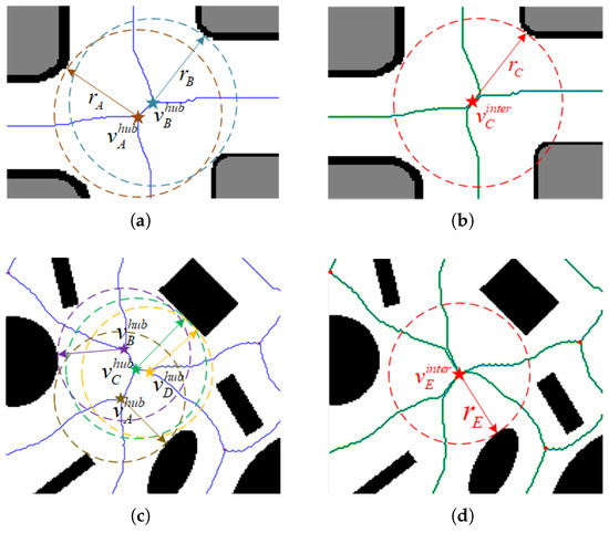
The distance field is used to calculate safety threshold radius of (indicated by the solid arrow in Figure 2) and the corresponding safety circle (indicated by the dashed circle in Figure 2), defined as the distance between each hub node and its nearest obstacle. When two neighboring HNs are within each other’s safety threshold radius, they are classified as close HNs, denoted as:
Figure 2.
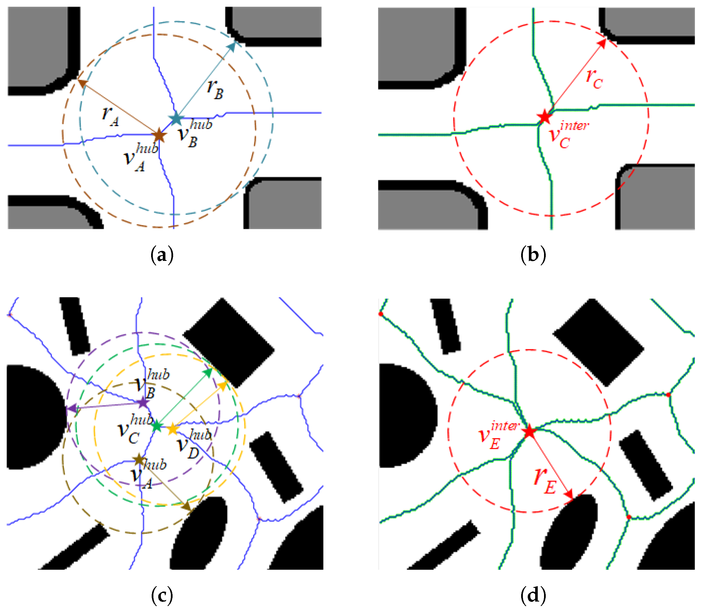
Merging close HNs. (a) Single-neighbor close HNs. (b) Merging into a IN. (c) Multiple-neighbor close HNs. (d) Merging into a IN. In (a,c), stars represent the HNs, arrows denote the distance to the nearest obstacles, and blue lines represent the skeleton paths before merging. In (b,d), red stars represent the INs obtained after merging, arrows denote the distance to the nearest obstacles, and green lines represent the merged skeleton paths. According to Algorithm 1, the process from (a) to (b) requires only one iteration, whereas the process from (c) to (d) requires three iterations.
And based on Equation (2), every HN can be determined whether it belongs to the close HN pairs
It can be observed that, based on Equation (1), a close HN may have one (Figure 2a) or multiple (Figure 2c) neighbors in . Then, close HNs in the same area should be merged into a IN recursively. Algorithm 1 presents the procedure for generating the STSG, where represents the construction of close HN pairs by Equation (1), denotes the process of node merging based on the centralization method, refers to the process of maintaining the neighbor-edge relationships for the newly generated nodes, and describes the removal of old nodes and edges information from the graph. Figure 2a,b presents the merging result of single-neighbor close HNs, whereas Figure 2c,d depicts the result of the iterative merging of multiple-neighbor close HNs.
3.2. The Construction of Smooth Corridor Edges
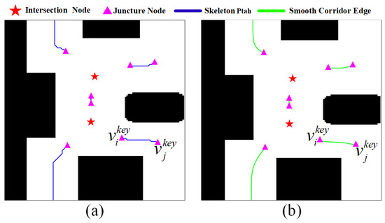
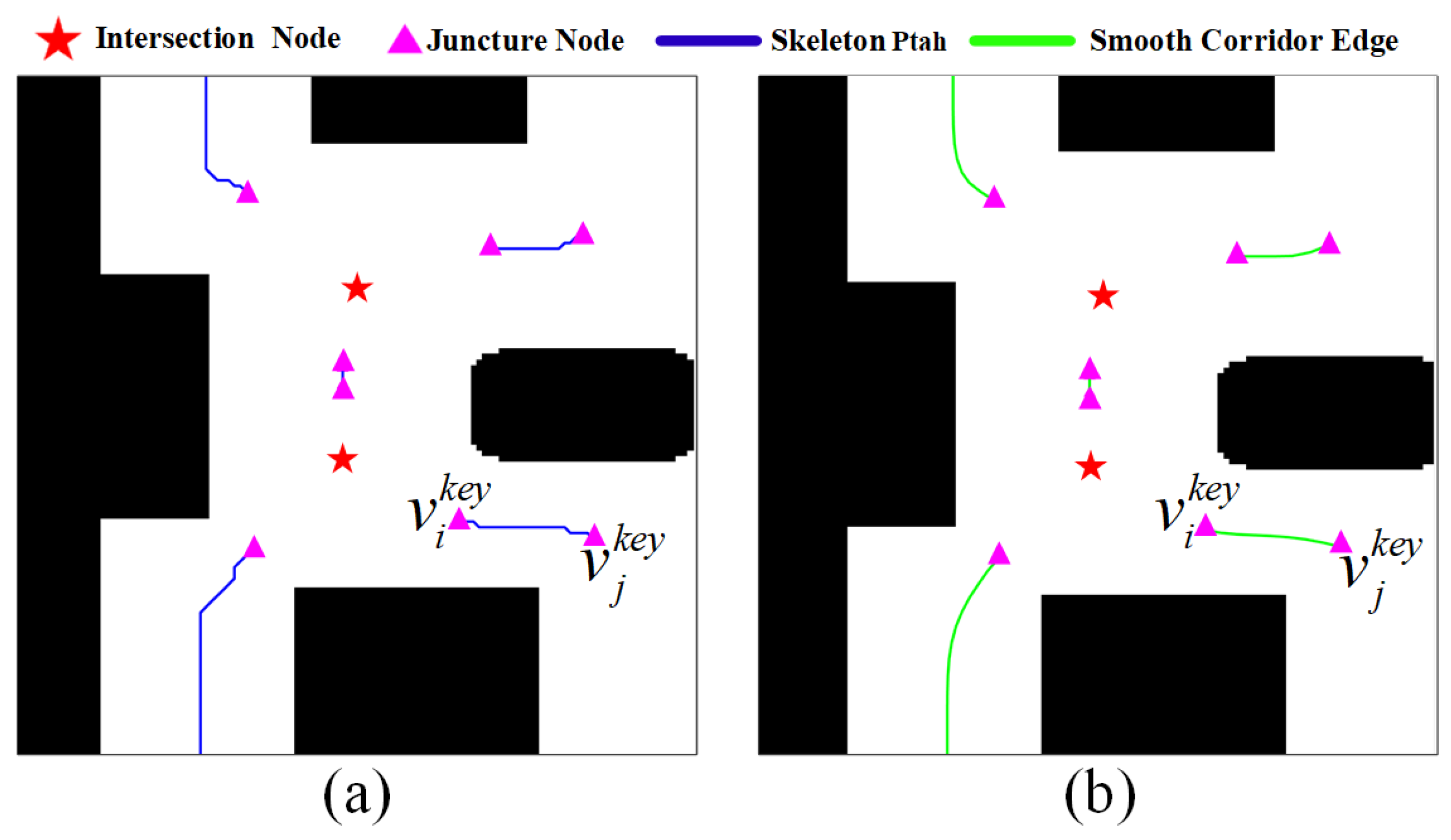
Based on the STSG, the JNs at each intersection are first identified. A constrained optimization-based B-spline is then applied to refine the connection between two JNs on the same edge, thereby generating a smooth road segment, as illustrated by the blue path in Figure 1l.
3.2.1. JNs Identification
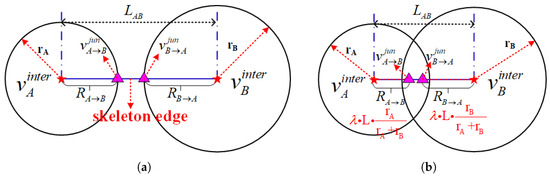
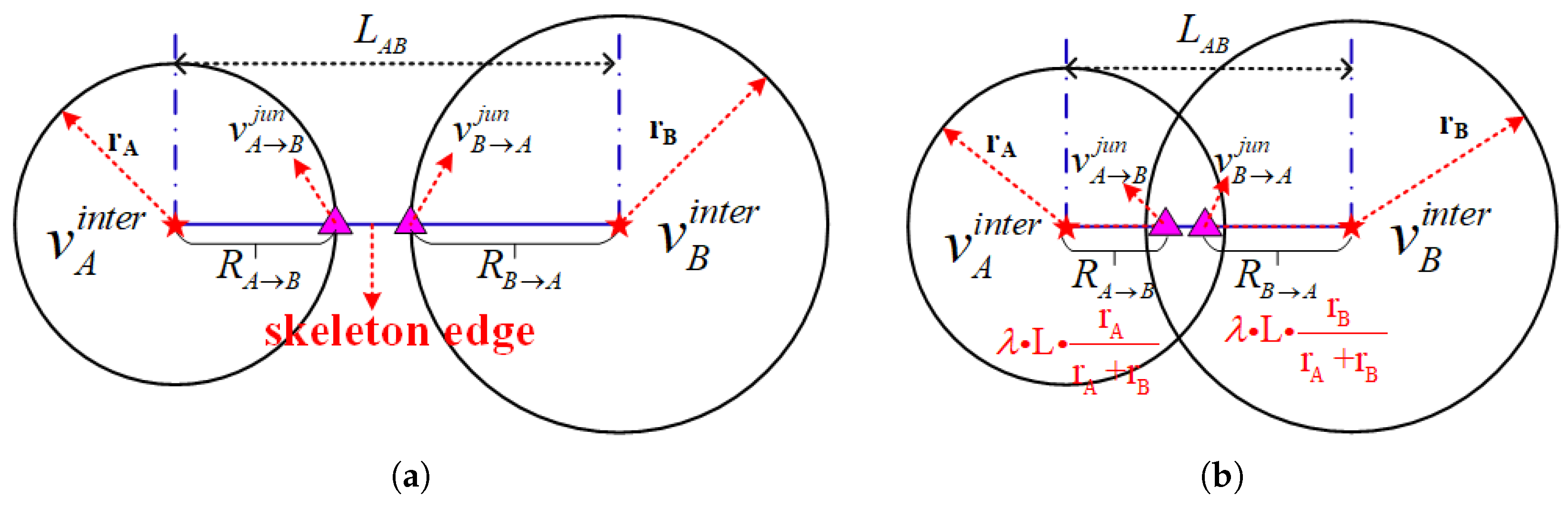
The JNs are are determined by identifying the intersection between skeleton paths in and a circle with a junction radius centered at each IN. For neighboring INs, the junction radius is computed under two different cases, as illustrated in Figure 3, based on the distance between the two INs and their safety radius of each IN, and is defined as:
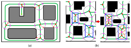
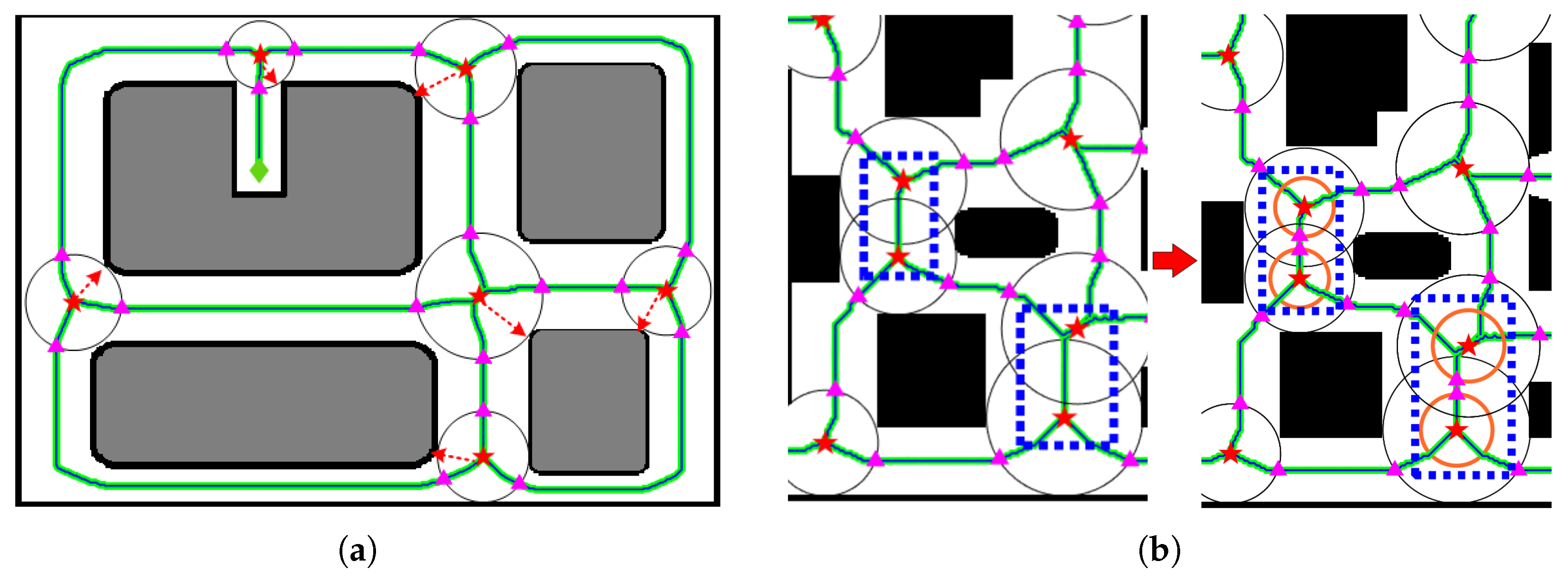
where , , and controls the scale of neighboring INs, can be heuristically set within the range . In the subsequent experiments of this paper, is set to 0.8. Figure 4 presents the JN identification results corresponding to Figure 3.
Figure 3.
Identification of the JNs. (a) Case 1: neighboring INs are sufficiently separated, and the junction radius is set equal to the safety radius of each IN. (b) Case 2: neighboring INs are close, their safe regions overlap. To ensure valid JNs, the junction radius is defined as a weighted function of the distance between the two INs. The meanings of the lines, arrows, triangles, and stars are the same as those in Figure 1.
Figure 4.
Examples of JN identification. (a) Case 1: a simple environment in which the distance circles of two INs do not intersect, corresponding to Figure 3a. (b) Case 2: two nearby distance circles overlap, as highlighted by the blue dashed rectangle, corresponding to Figure 3b. The meanings of the symbols and legends are the same as those in Figure 1.
Subsequently, the set and are constructed. The skeleton path within the corridor region between neighboring KNs belonging to different intersections can then be directly obtained, and is denoted as .
| Algorithm 1: STSG Generation |
| Input: , Distance field map |
| Output: |
|
3.2.2. Constrained Optimization-Based B-Spline Curves
The corridor skeleton path extracted from the road graph consists of piecewise linear segments connected at discrete nodes, as illustrated by the blue paths in Figure 5a. Such paths are not directly suitable for robot tracking because they contain sharp corners, discontinuous curvature, and may violate vehicle kinematic constraints. Therefore, a trajectory smoothing and optimization step is required to transform the discrete skeleton path into a continuous and dynamically feasible trajectory. This section proposes a method to generate SCEs using B-spline interpolation, optimizing for smoothness while enforcing curvature and safety constraints.
Figure 5.
Smoothing of corridor edges. (a) Corridor edge before smoothing. (b) Corridor edge after smoothing.
A B-spline curve can locally adjust a path without altering its overall shape, making it well suited for path smoothing. Given n + 1 control points, which define the direction and boundary range of the spline curve, the k-th order B-spline curve is given by the following definition:
where is the i-th B-spline basis function whose order is corresponding to the control point and u is the variable. The basis function has the following derivation formula:
To balance path smoothness and computational efficiency, a third-order quasi-uniform B-spline () is adopted. A cubic B-spline guarantees continuity of the generated trajectory, ensuring continuous curvature and smooth steering for mobile robots. Lower-order splines cannot guarantee curvature continuity, while higher-order splines introduce unnecessary computational complexity and may lead to overfitting. Therefore, the cubic B-spline provides a practical trade-off between smoothness and efficiency for real-time path generation. When selecting control points along the skeleton path between key nodes (KNs) on the same edge, sparse sampling is applied in smooth regions, whereas denser sampling is used in high-curvature regions. This strategy ensures that the smoothed path closely follows the overall trend of the skeleton.
Let denote the path to be optimized, which is generated through B-spline interpolation. The objective is to minimize a cost function that incorporates terms related to path smoothness, curvature constraints, and safety penalties. The objective function is defined as:
The first term ensures path smoothness by minimizing the curvature, represented by the second derivative of the trajectory. The second term imposes an upper bound on the instantaneous curvature of the trajectory at each node, ensuring compliance with the vehicle’s non-holonomic constraints. is the change in the tangential angle at the vertex. Here, is the maximum allowable curvature of the path, and is a quadratic penalty term. The third term penalizes potential collisions with obstacles, where is a quadratic penalty term, denotes the location of the obstacle closest to the vertex, and is the threshold for the maximum effective range of distance to obstacles. , , are weights. In the following experiments, we use a differential-drive robot (with zero minimum turning radius) and set , where denotes the physical radius of the robot and denotes the grid-map resolution. Meanwhile, we empirically set , , and , and keep them fixed across all scenarios. Finally, the gradient descent algorithm can be employed to solve this problem and obtain smooth road sections. Figure 5 presents a comparison of the optimized and unoptimized corridor edges in a local map, where the optimization process significantly enhances the skeleton path between neighboring KNs. As a result, the set of SCEs, , is constructed, where , are located at different intersections and represents the proposed B-spline smoothing algorithm.
3.3. The Construction of Smooth Intersection Edges
In this section, SIEs are constructed between the neighboring JNs within the same intersection, ensuring tangential continuity at the JNs, as well as maintaining rationality and safety within the intersection region. To address the Hermite interpolation problem, the Clothoid-based approach is adopted, ensuring gradual directional changes along the curve and making it easier for robot tracking and control.
Assuming the initial coordinate of the curve is , the Clothoid can be defined by the following equation according to the Fresnel integral function:
where s is the arc-length parameter, is a parameter controlling the rate of change of curvature, is a parameter that controls the initial curvature, and is an offset constant.
The curvature and tangent angle of any point on the curve can be described as:
continuity fitting based on the convolutional curve [26] is employed to ensure tangential continuity at the JNs, providing a seamless geometric connection and maintaining the overall smoothness of the design.
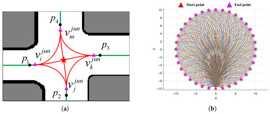
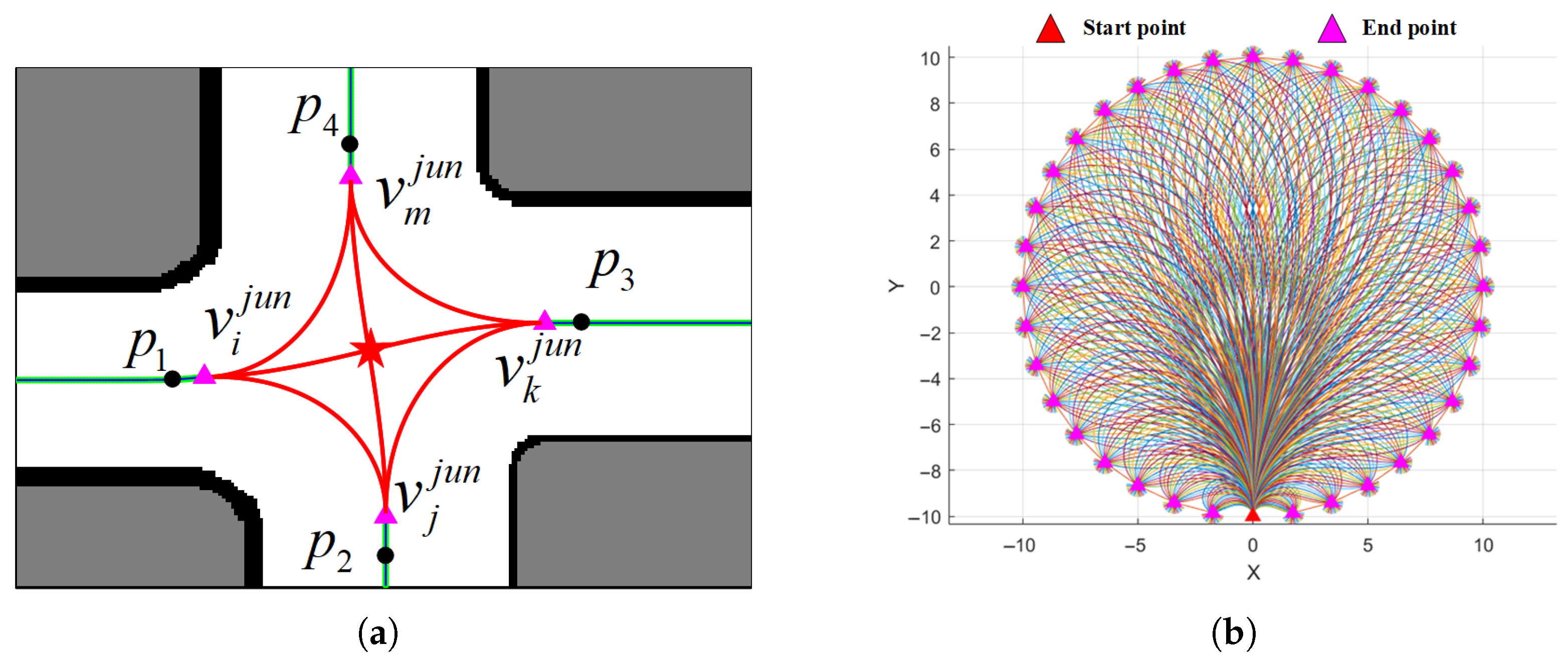
As a result, the set of SIEs is constructed as , where , are junction nodes located within the same intersection and denotes the proposed clothoid-based smoothing operator. As an illustrative example, the SIEs between neighboring JNs within the same intersection are shown in Figure 6a. The start and end points of each SIE coincide with the corresponding JNs, and the initial direction is determined by the tangent vector at the endpoint of the smooth corridor edge.
Figure 6.
Intersection modeling. The meanings of the symbols and legends are the same as those in Figure 1. (a) Clothoid-based SIEs constructed between JNs within an intersection. (b) Monte Carlo sampling results illustrating that the generated SIEs remain within the intersection boundary.
To verify collision-free motion, Monte Carlo sampling is employed to demonstrate that the proposed SIEs do not extend beyond the boundary of the intersection circle. Specifically, a circle is generated with a center of (0,0) and a radius of 5 m. Start point (0, −10), ending at any discrete point on the circle, with a direction of , where a is the direction from the center of the circle to the end point. After fitting and smoothing, the result shown in Figure 6b clearly demonstrates that the curve will not cross any obstacles, as it remains within the area of the circle. Finally, HTMRG is constructed and represented as , where W denotes the distance-based cost between neighboring KNs.
4. The Application of HTMRG
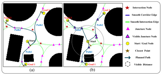
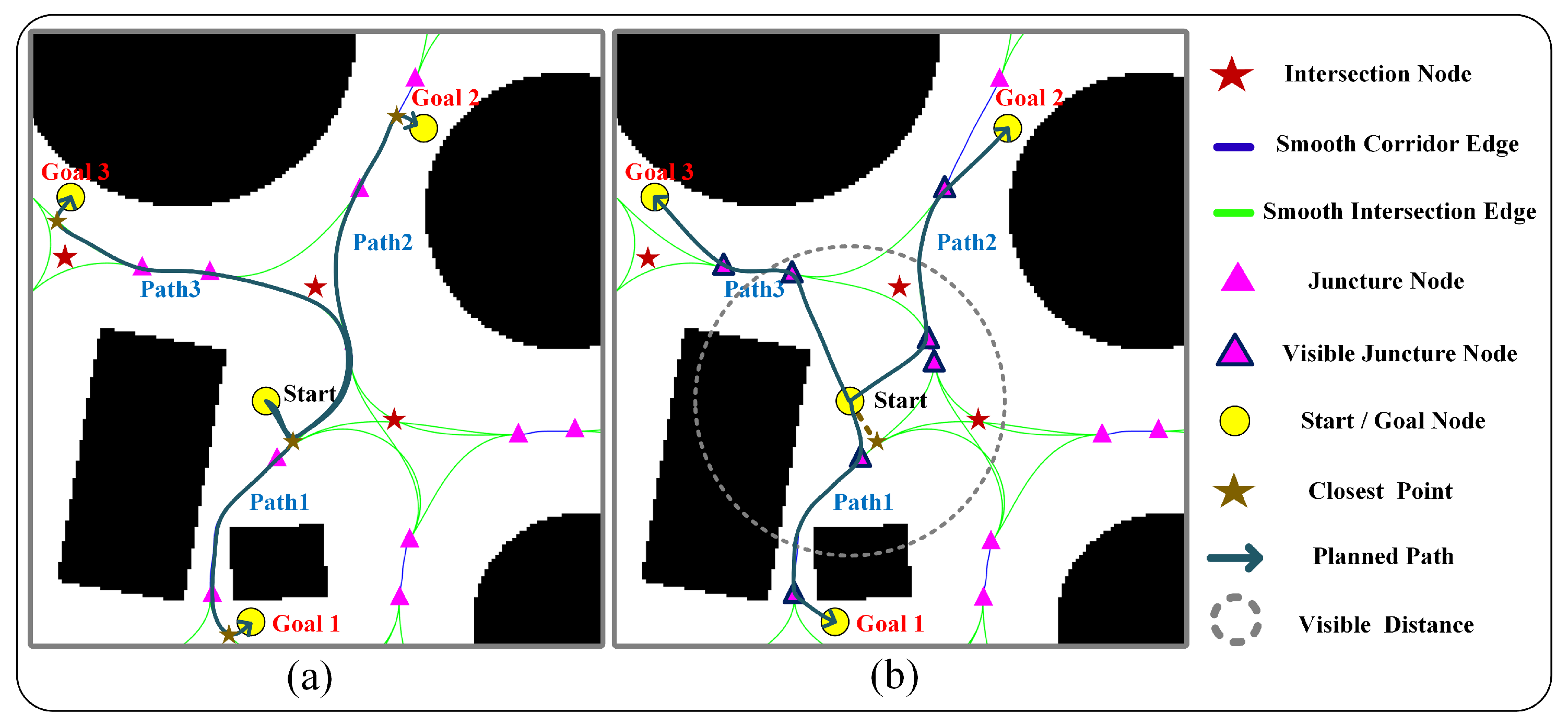
To perform path planning on the HTMRG, the start and goal nodes must be inserted into the graph prior to graph search. A typical approach identifies the skeleton points closest to the start and goal locations, connects them to the graph, and then performs a search [22]. However, as shown by Path2 and Path3 in Figure 7a, this method can lead to suboptimal paths. In contrast, Figure 7b shows improved results achieved using the proposed insertion strategy.
Figure 7.
Comparison of node insertion strategies. (a) Traditional insertion method based on the nearest neighbor point. (b) Proposed insertion method enabling more reliable path connections based on visible connections.
Accordingly, we propose a strategy to insert the start and goal nodes into the HTMRG by leveraging the visibility (line-of-sight) relationship between the newly inserted node and the KNs. Taking the insertion of the start node as an example, the graph after the insertion of the new node, denoted as , is presented in Algorithm 2. The process for inserting the goal node is similar.
| Algorithm 2: Inserting Node into HTMRG |
| Input: Start node , , Obstacle |
| Output: |
|
In Algorithm 2, denotes a visible node from the node to be inserted. The condition denotes that the line between the node to be inserted and the visible node does not intersect any obstacles. The constraint restricts candidate visible nodes to those within a distance threshold of the node to be inserted. In the subsequent experiments, is set to half of the map diagonal length. Moreover, denotes the point closest to the RG from the node to be inserted. It is important to note that during the insertion of the start or goal nodes into the RG, the smoothness of the newly inserted segments is not considered, as these segments are generally short and can be managed by local planning in the robotic system.
After inserting both the start and goal nodes, the augmented graph is obtained. Finally, the Dijkstra algorithm is used to search for the path between the start and goal nodes in , taking into account the path length between KNs. Figure 1m illustrates the path planning results using the proposed insertion method, demonstrating the effectiveness, safety, and smoothness of the approach.
5. Simulation Experiments
5.1. Simulation Overview in MATLAB
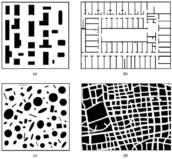
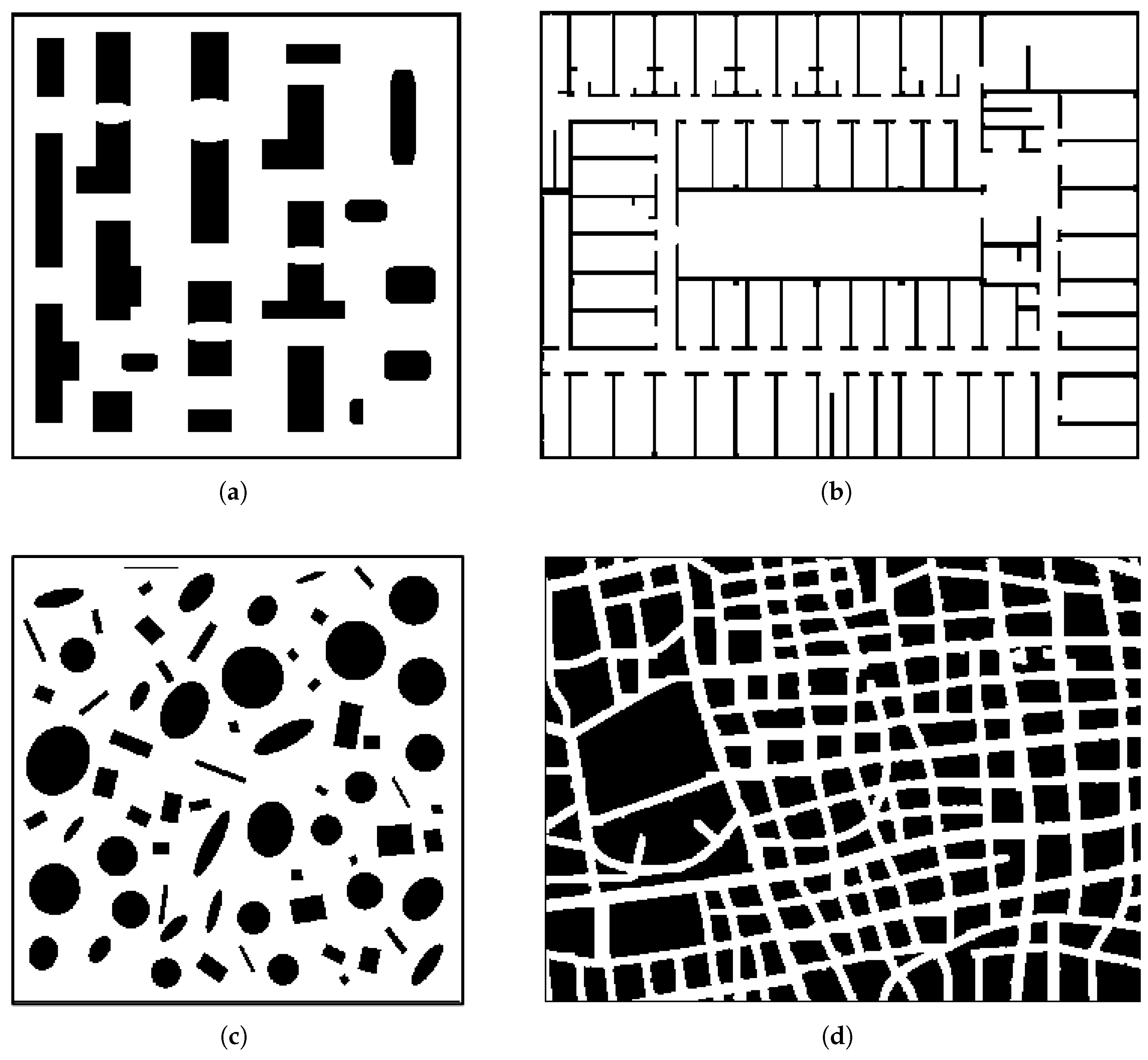
Four grid maps were used as the simulation maps (Figure 8), each containing the following specific information:
Figure 8.
Simulation maps used in the experiments. (a) Map 1: Structured environment. (b) Map 2: Indoor environment. (c) Map 3: Chaotic environment. (d) Map 4: Block environment.
- (a) Map 1: Structural scenario, 500 × 500 (pixels).
- (b) Map 2: Indoor scenario, 796 × 598 (pixels).
- (c) Map 3: Chaotic scenario, 900 × 900 (pixels).
- (d) Map 4: Block scenario, 796 × 598 (pixels).
5.2. Simulation Results and Comparative Analysis
5.2.1. The Results of HTMRG
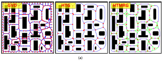
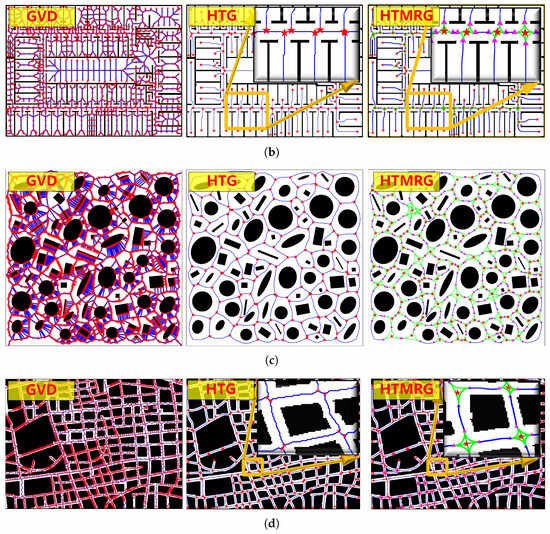
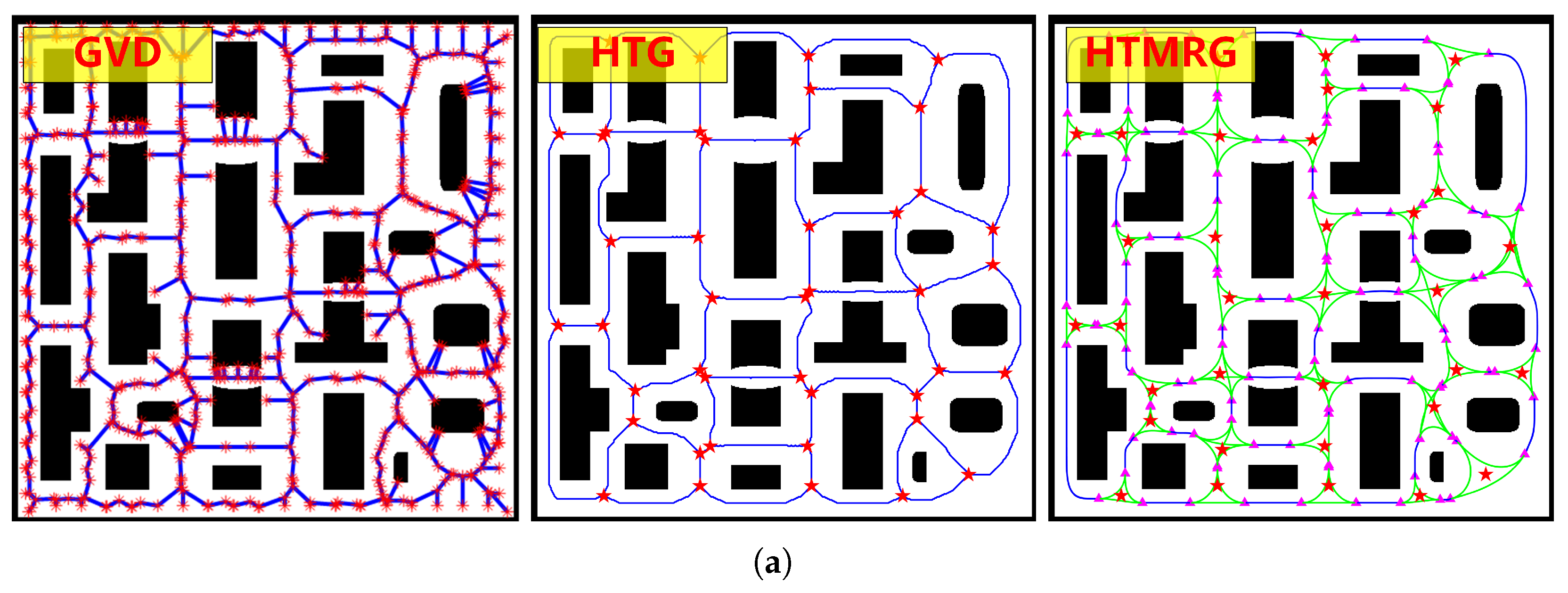
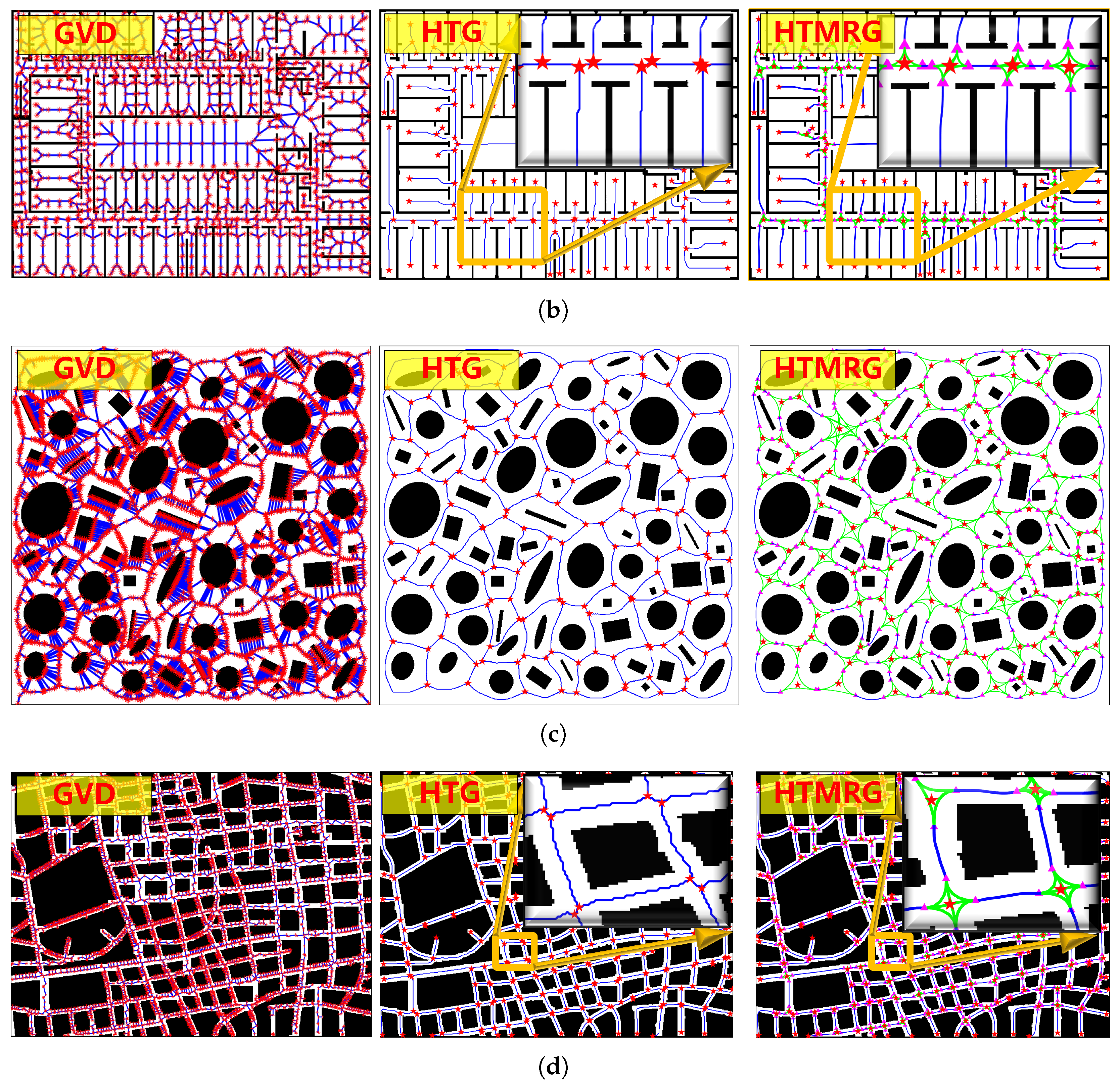
The proposed HTMRG is compared with the Generalized Voronoi Diagram (GVD) [27] and the Hierarchical Topology Graph (HTG) [28]. Figure 9a–d present qualitative comparison results across four different types of map representations. The GVD is characterized by a large number of nodes with rough and irregular connections. While the HTG reduces the number of nodes compared to GVD, it still contains redundant INs, and its connections lack smoothness.In contrast, HTMRG eliminates redundant nodes and provides smooth connections between SCEs and SIEs, achieving a compact structure with sufficient topological expressiveness and efficient navigability.Moreover, these results demonstrated that the proposed method is capable of handling a wide range of application scenarios, offering strong adaptability to diverse environments.
Figure 9.
Visual comparison of GVD, HTG, and HTMRG. The meanings of the symbols and legends are the same as those in Figure 1. (a) Map 1—Structural scenario. (b) Map 2—Indoor scenario. (c) Map 3—Chaotic scenario. (d) Map 4—Block scenario.
5.2.2. Comparison of Inserting Methods Based on HTMRG
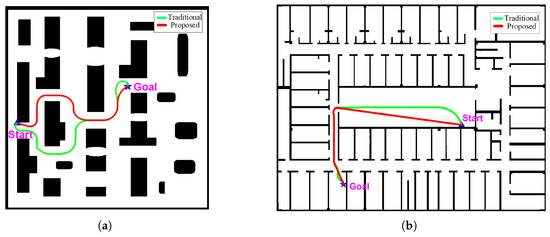
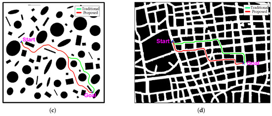
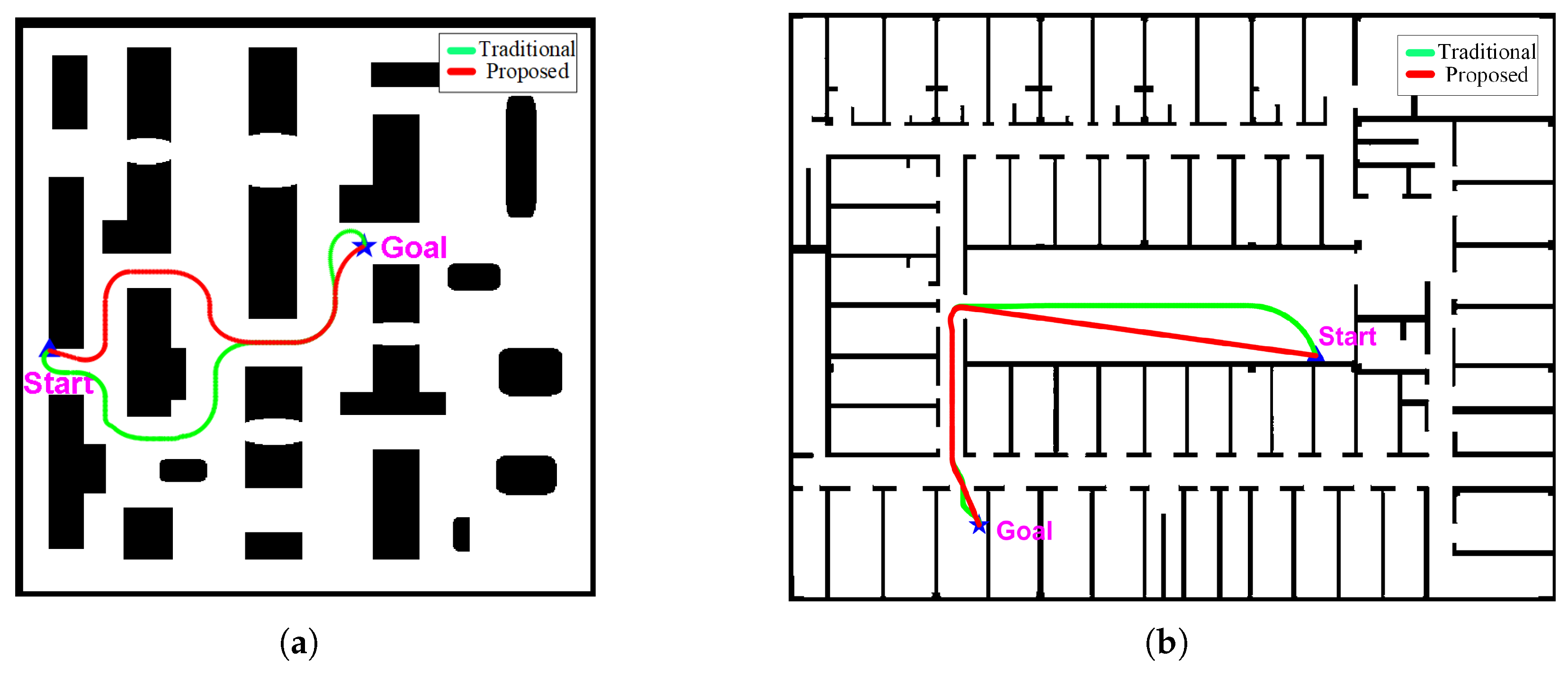
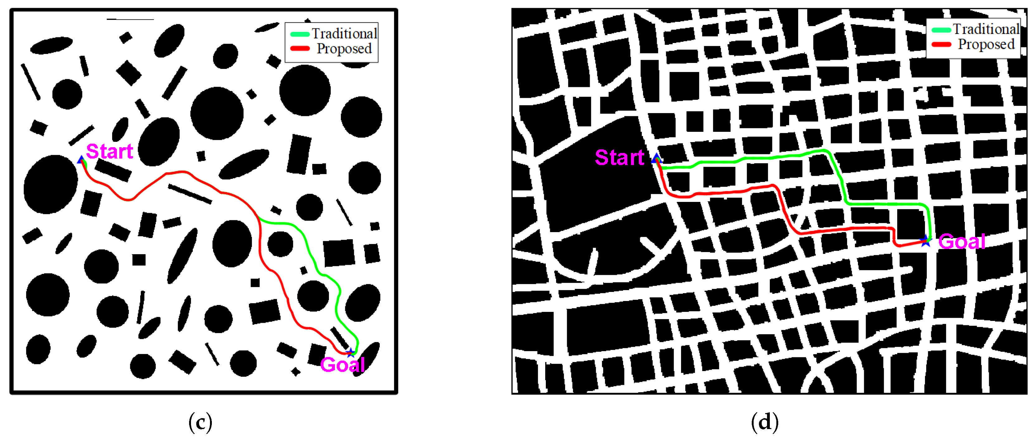
To validate the effectiveness of the proposed insertion method on HTMRG, 50 start–goal pairs were randomly generated in the free space of each of the four maps. To avoid trivial cases, the Euclidean distance between the start and goal was required to be greater than half of the longer map dimension, and the start and goal were not mutually visible. For each start–goal pair, both the traditional shortest-distance insertion method and the proposed insertion method were applied, and the planned path length was recorded. We report the mean and standard deviation of the path lengths and perform a paired statistical test to assess the significance of the improvement. As shown in Table 1, the proposed insertion approach consistently reduces the planned path length across all maps. Specifically, the average path length is reduced by 6.99%, 4.55%, 4.13%, and 4.23% on Map 1–Map 4, respectively. The improvements are statistically significant on all maps, with p-values ranging from to . These results demonstrate that the proposed insertion strategy can effectively generate shorter and more reasonable paths by considering all feasible insertion scenarios. Figure 10 provides a qualitative comparison, where the red paths generated by the proposed method are more intuitive and shorter than the green paths produced by the traditional method.
Table 1.
Comparison of average path length under different insertion methods (pixels).
Figure 10.
Visual comparison of start–goal insertion methods in the HTMRG. The green paths correspond to the traditional shortest-distance insertion method, while the red paths correspond to the proposed insertion method. (a) Map 1. (b) Map 2. (c) Map 3. (d) Map 4.
5.2.3. Comparison of Path Planning on Different Graphs
To compare the path planning performance across different graph representations, 50 start nodes and 50 goal nodes were randomly selected on each map. To avoid trivial cases, the Euclidean distance between the start and goal was required to be greater than half of the longer map dimension, and the start and goal were not mutually visible. For each pair, a path was planned using the Dijkstra algorithm on the Grid, GVD, HTG, and HTMRG graphs. Table 2 reports the mean and standard deviation of the planning time over the 50 trials.As shown in Table 2, both HTG and HTMRG significantly reduce the planning time compared with the Grid and GVD representations. For example, on Map 3, the average planning time decreases from ms (Grid) and ms (GVD) to ms (HTG) and ms (HTMRG). This substantial reduction is attributed to the hierarchical topology structure, which effectively reduces the search space and accelerates graph traversal. Compared with HTG, HTMRG exhibits slightly higher planning time across all maps, but remains in the same order of magnitude (within a few milliseconds difference), indicating that the enriched hierarchical topology representation introduces only minor computational overhead while preserving efficient search performance.
Table 2.
Comparison of average path planning time on different graphs representations (ms).
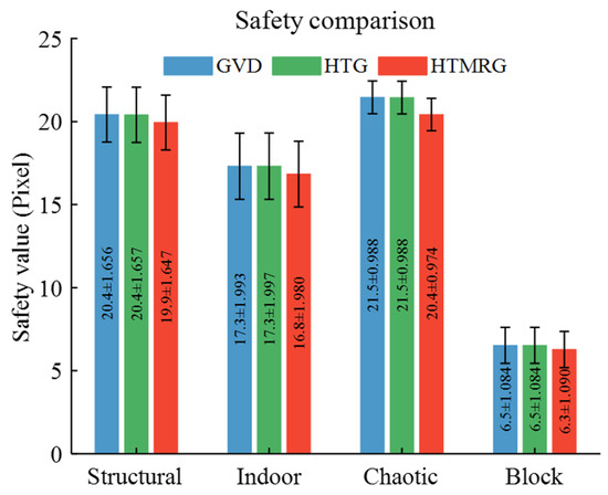
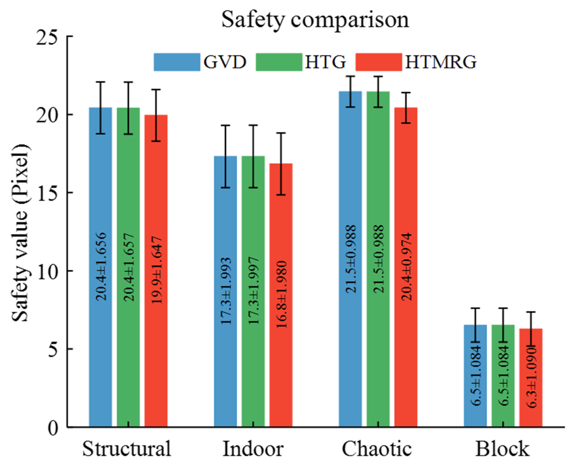
In addition, quantitative comparisons of average path length, curvature, and safety clearance were conducted to further evaluate the performance of the proposed algorithm.
The average discrete curvature of each path is defined as:
where denotes the total number of path points, represents calculating the curvature of point based on the circumcircle of three points.
The average safety clearance is defined as:
where represents the nearest Euclidean distance from to the surrounding obstacles, which can be directly acquired from the distance field graph.
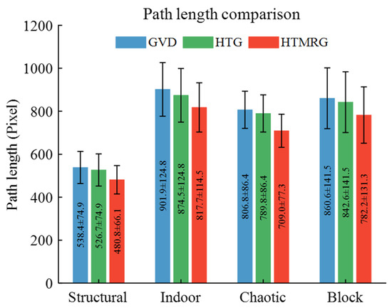
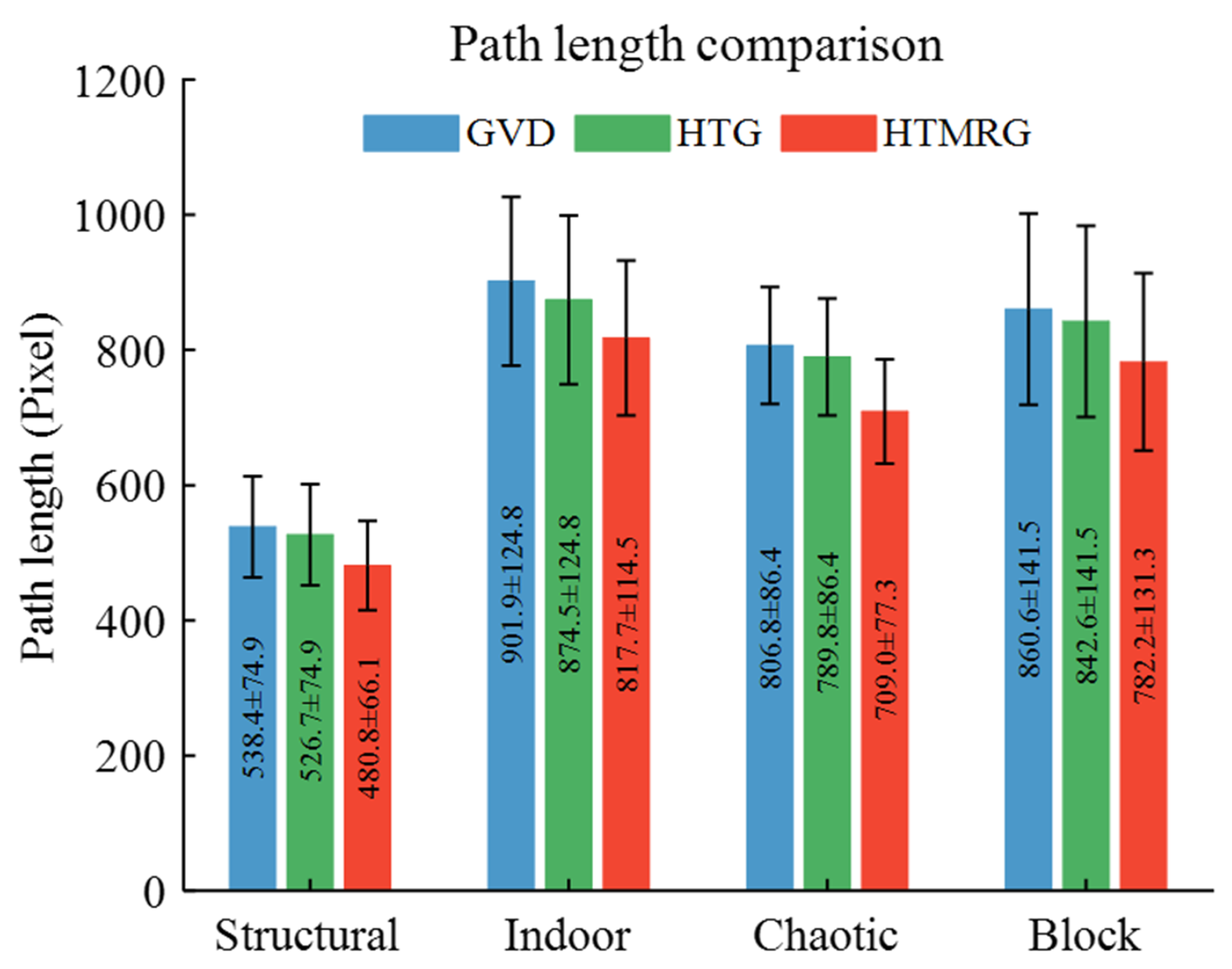
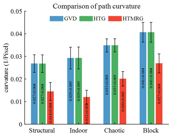
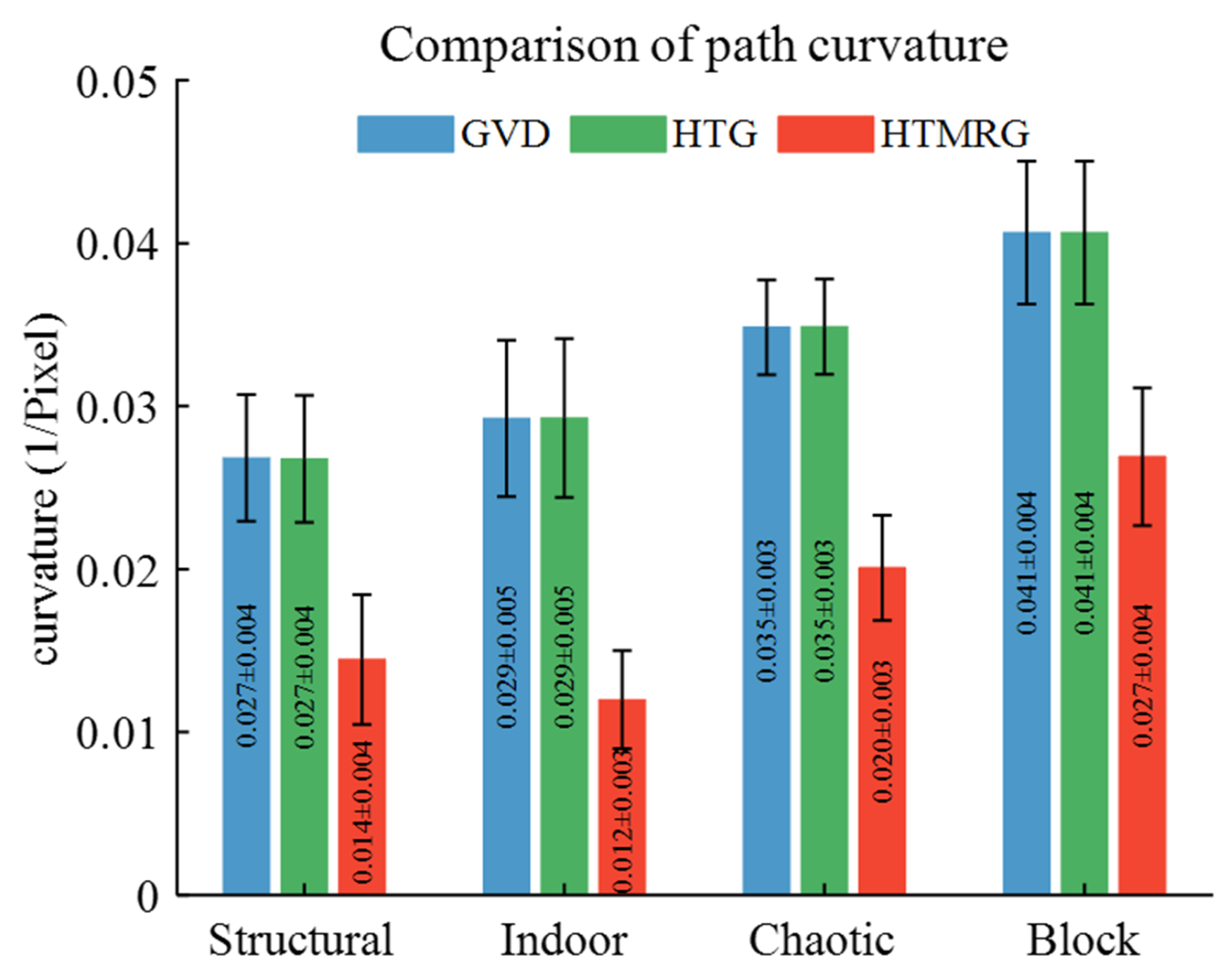
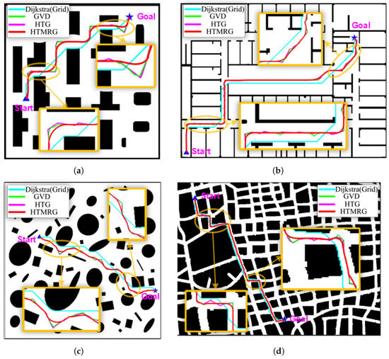
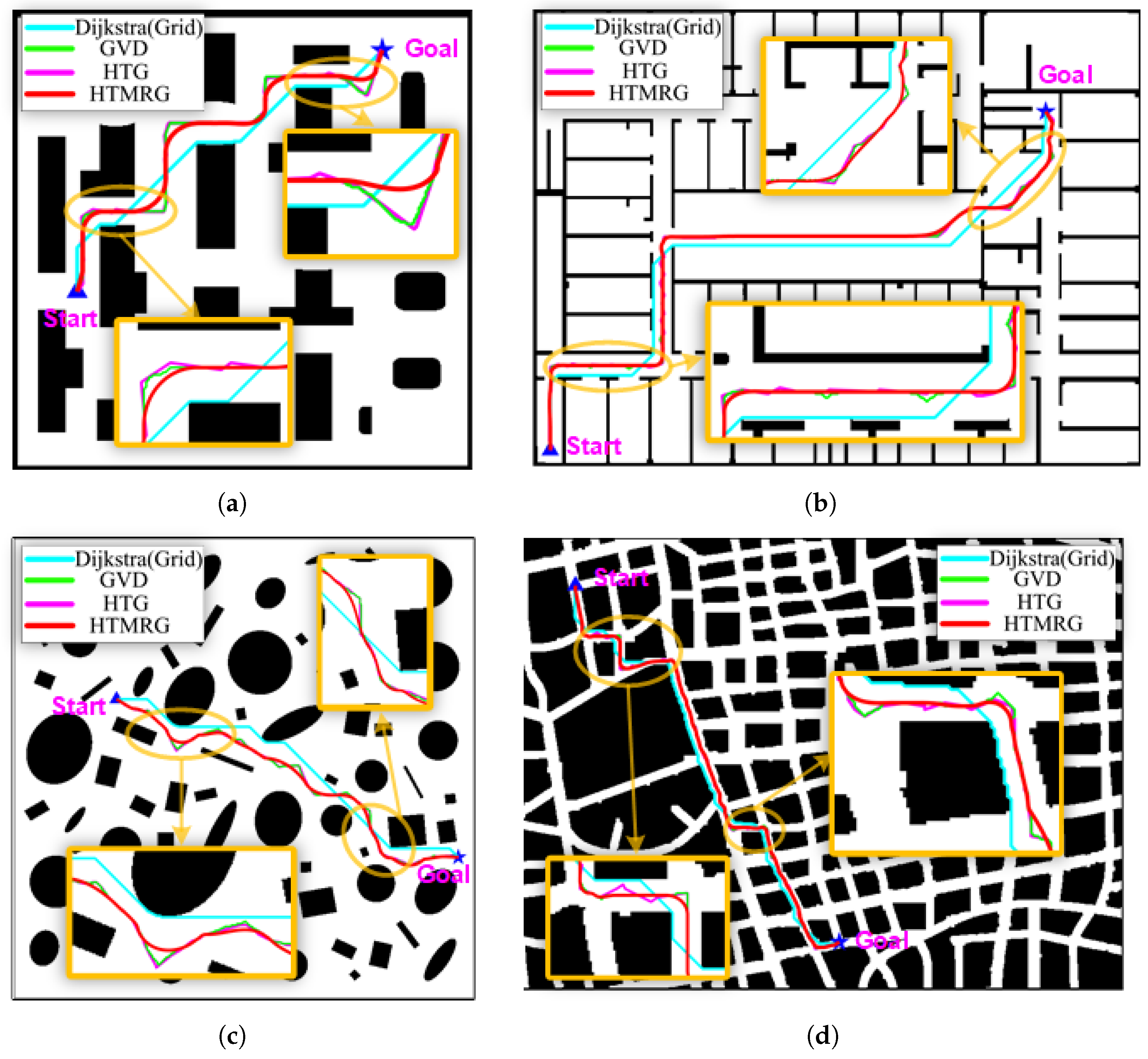
The paths planned using the proposed HTMRG structure, as shown in Figure 11, Figure 12 and Figure 13, demonstrate reduced path length, improved smoothness, and consistent safety levels. Figure 14 presents representative results across four different maps. Compared to paths generated using Grid, GVD, and HTG methods, those planned on HTMRG are smoother and exhibit fewer twists and turns, owing to the integration of SCEs and SIEs.
Figure 11.
Comparison of average path length across different environments on different graphs representations.
Figure 12.
Comparison of curvature comparison across different environments on different graphs representations.
Figure 13.
Comparison of safety comparison across different environments on different graphs representations.
Figure 14.
Visual comparison of path planning results using different graph representations. Paths are generated using Dijkstra’s algorithm on the Grid, GVD, HTG, and HTMRG. (a) Map 1. (b) Map 2. (c) Map 3. (d) Map 4.
5.3. Gazebo Simulation in ROS
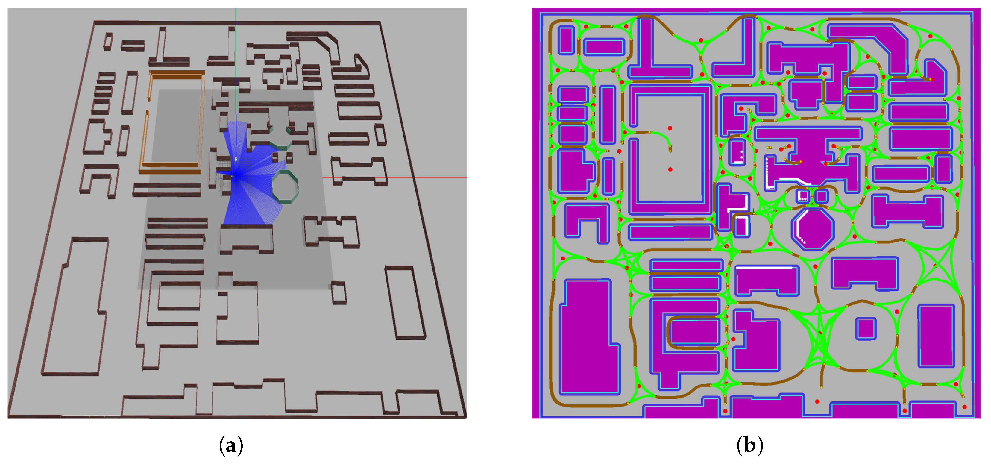
The proposed method was integrated into the ROS framework and evaluated in the Gazebo simulation environment, as shown in Figure 15a. The simulated environment represents a composite scenario containing both sparse and dense regions, structured and unstructured areas, as well as open and semi-enclosed spaces. Gmapping SLAM and the OctoMap package were employed to generate the occupancy grid map. The resulting grid map has a resolution of 0.1 m per pixel and a size of 897 × 957 pixels. The grid-map resolution (granularity) has a direct impact on the complexity and accuracy of the constructed road graph. In practice, the grid resolution is selected according to the robot size and is typically set to approximately one-half to one-quarter of the robot radius, which provides a balance between safety and efficiency.
Figure 15.
Gazebo-based simulation results. (a) Gazebo simulation environment. (b) HTMRG constructed from the generated occupancy grid map. The green lines represent SIEs, the brown lines represent SCEs, and the red dots denote the INs.
Figure 15b illustrates the constructed HTMRG, where red dots represent INs, green dots indicate SIEs, and yellow lines denote SCEs. The HTMRG structure clearly demonstrates its effectiveness in systematically constructing a functional road network for the environment.
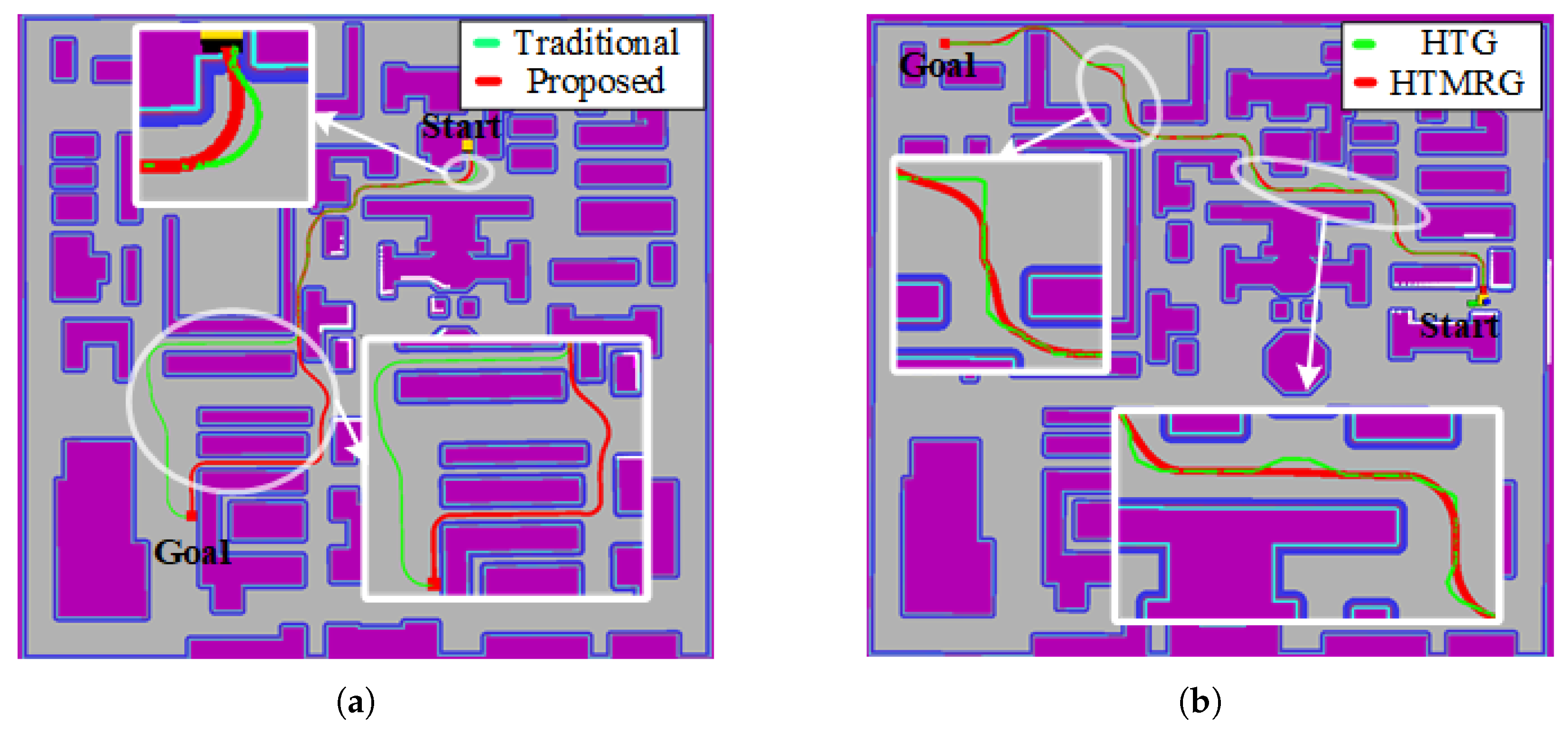
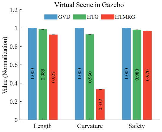
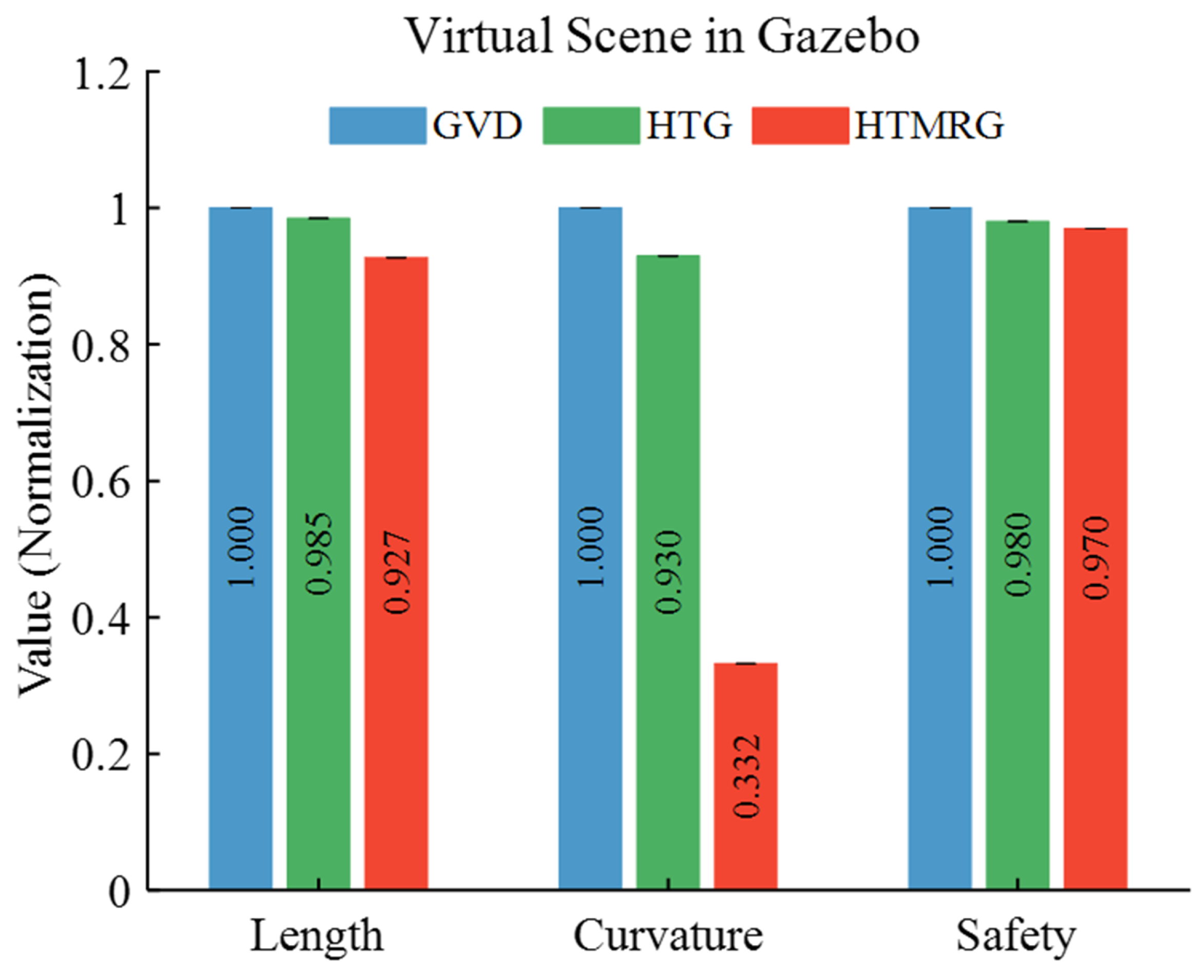
As shown in Figure 16a, the proposed insertion strategy reduces the average path length by 4.02% compared with the traditional insertion method, evaluated over 30 randomly generated start–goal pairs in the Gazebo environment. Additionally, as shown in Figure 17, path planning with HTMRG achieves shorter path lengths, improved smoothness, and enhanced safety compared to SG and HTG. Figure 16b illustrates a comparison of the intuitive path outputs generated by HTG and HTMRG, highlighting the smoother and shorter paths produced by the proposed method. These results further validate the effectiveness of the proposed method in realistic simulation scenarios.
Figure 16.
Comparison of path planning results in the Gazebo environment. (a) Comparison of different start–goal insertion methods. (b) Path planning results on HTG and HTMRG.
Figure 17.
Performance comparison of different graphs representations.
6. Real Experiments
In this section, the proposed HTMRG-based path planning method is integrated into a UGV system for experimental validation in a real campus environment. The complete system includes localization, mapping, path planning, and motion control modules.
6.1. Experimental Environment and Conditions
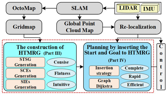
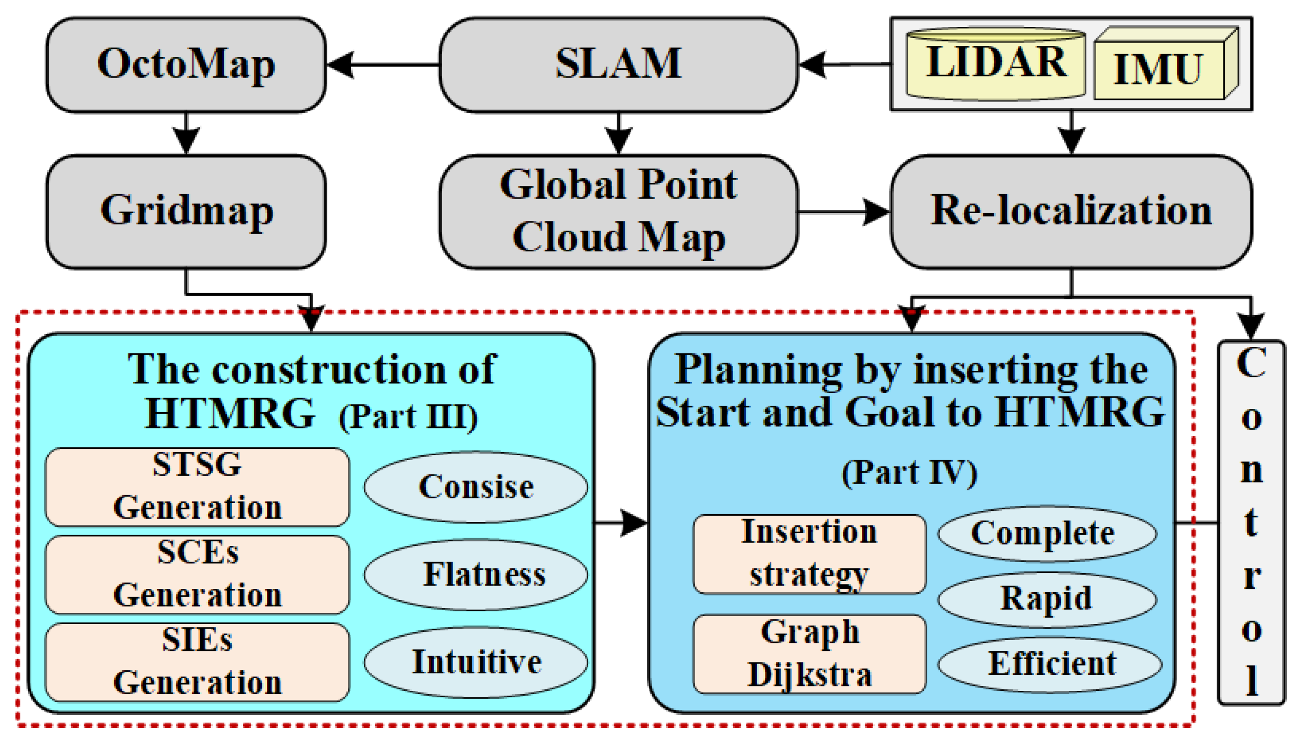
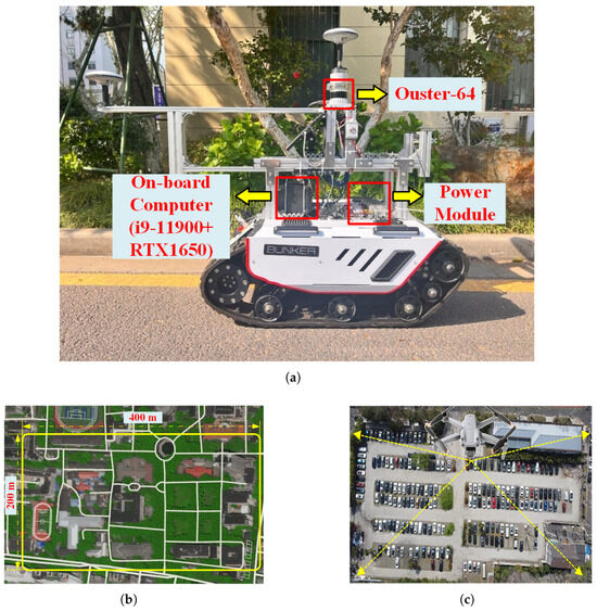
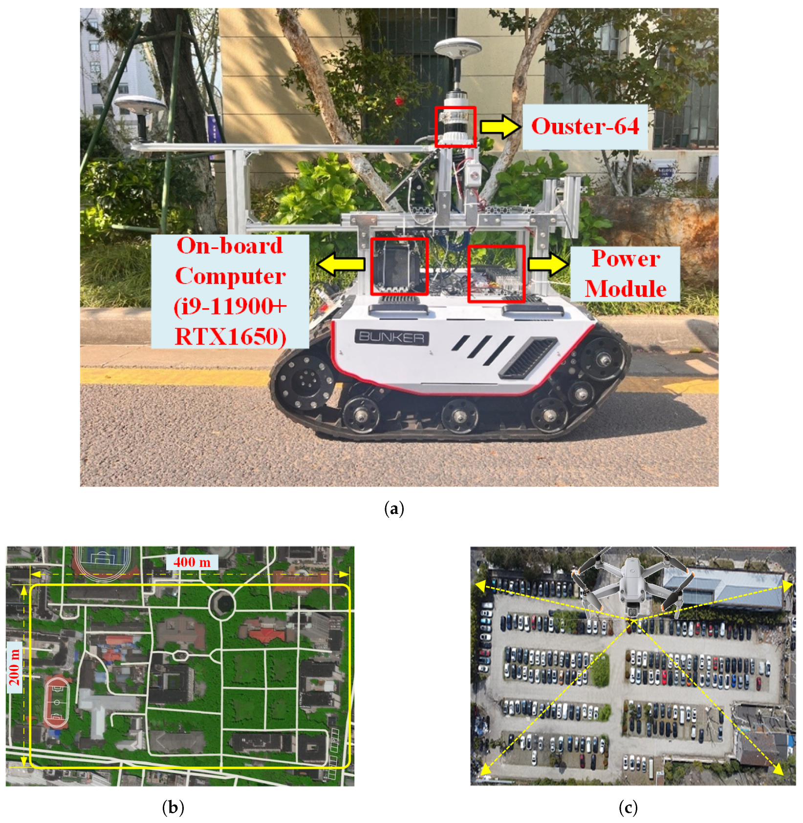
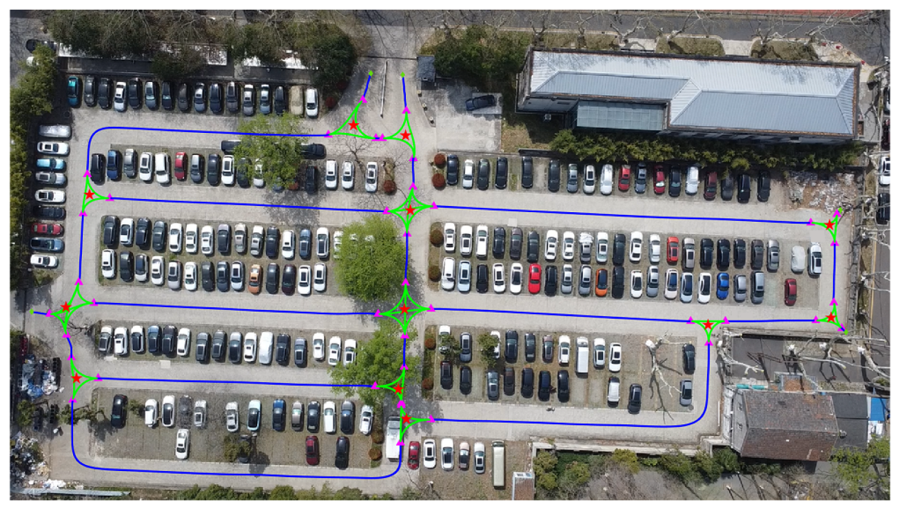
An autonomous navigation system for a UGV platform was developed, as shown in Figure 18. Figure 19b presents a section of the actual campus environment, measuring 400 m in length and 200 m in width. The tracked differential-type UGV platform, shown in Figure 19a, was equipped with an onboard computer (i9-11900) and an Ouster-64 LiDAR. The robot adopts a tracked skid-steering locomotion mechanism, which enables robust operation on uneven outdoor terrain. The platform has an approximate size of (length × width × height) and a maximum driving speed of . Due to the skid-steering configuration, the vehicle has a near-zero minimum turning radius, allowing in-place rotation.The onboard computer communicated with the chassis control board via the CAN bus. First, a global point cloud map was constructed using Lio-Sam [29]. Simultaneously, a grid projection with a resolution of 0.2 m was performed to produce a grid map. Noise removal was then applied to the global grid map. Online re-localization [30] within the prior map was then performed to estimate the robot pose. In addition, Figure 19c illustrates another experimental scenario in which a drone captures an overhead view of a parking lot, which is subsequently modeled and used for HTMRG construction.
Figure 18.
Overview of the UGV system architecture based on HTMRG.
Figure 19.
Real-world experimental setup. (a) Tracked UGV platform equipped with an onboard computer and a 64-beam LiDAR. (b) Campus test site (approximately 400 m × 200 m). (c) UAV aerial view of the parking lot used for overhead mapping.
6.2. Real-World Experimental Results and Comparative Analysis
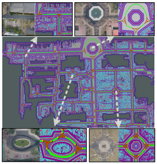
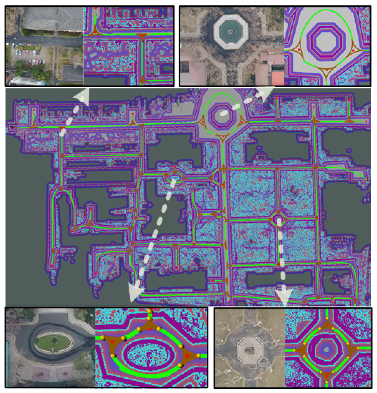
The HTMRG results for the campus and parking lot environments are depicted in Figure 20 and Figure 21, respectively. For the parking-lot scenario, the UAV overhead imagery is processed to extract traversable regions prior to HTMRG construction, using either semantic segmentation or manual annotation. The results indicate that the proposed method successfully constructed a hierarchical and smooth road network structure in real-world environments. The planned paths can be directly used by the control module for trajectory tracking and guidance.
Figure 20.
HTMRG representation constructed for a real-world campus environment. The green lines represent SIEs, the brown lines represent SCEs, and the red dots denote the INs. The enlarged views highlight typical intersections and curved road segments.
Figure 21.
HTMRG representation constructed for a real-world parking-lot environment. The meanings of the symbols and legends are the same as those in Figure 1.
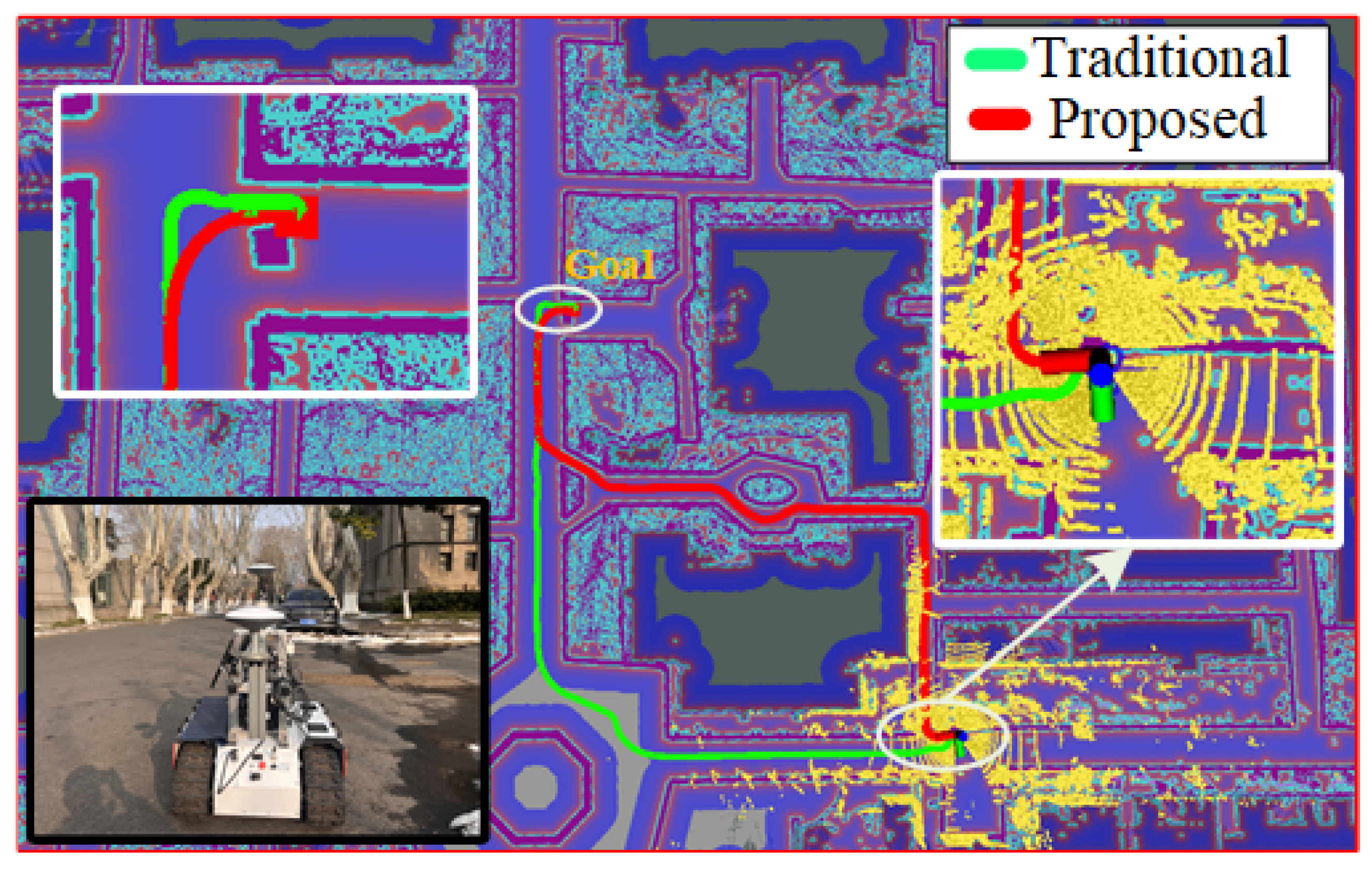
Inserting 20 start–goal pairs into the HTMRG shows that the proposed insertion method reduces the average path length by 4.36% compared to the traditional approach. Figure 22 presents a representative example: the path generated by the proposed method (red) is 192 m, whereas the path generated by the traditional method (green) is 208 m.
Figure 22.
Comparison of start–goal insertion methods in the HTMRG framework. The green path corresponds to the traditional insertion method, while the red path corresponds to the proposed insertion method.
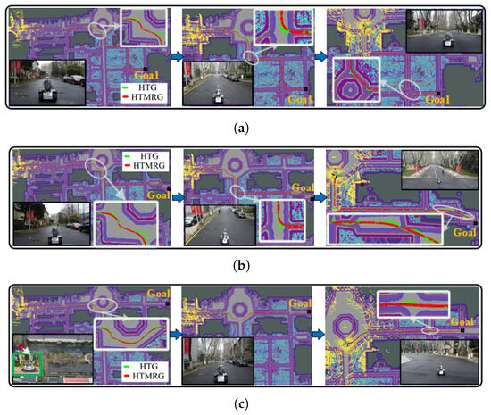
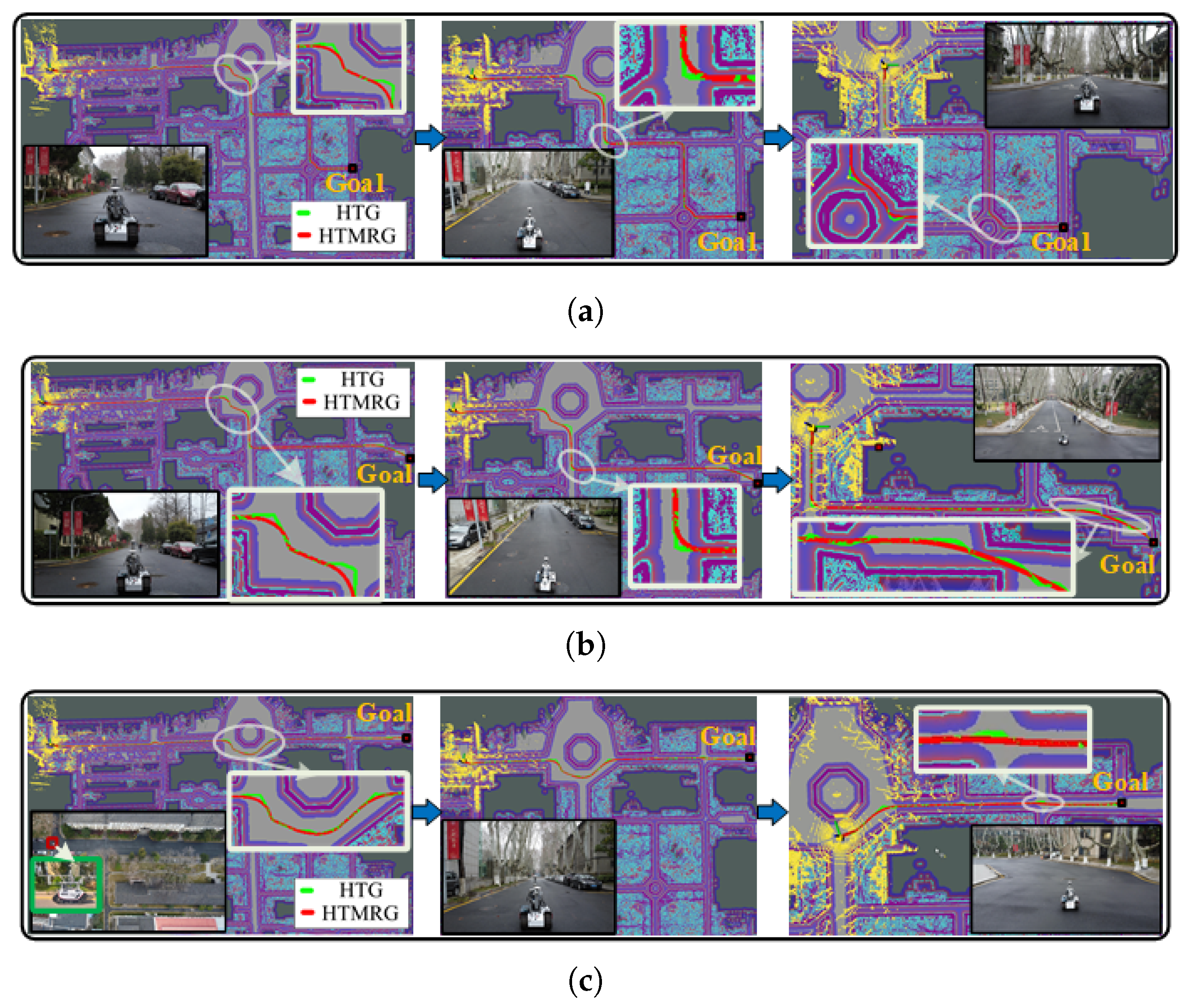
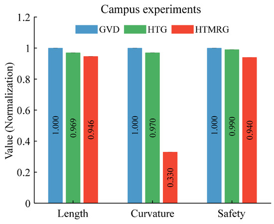
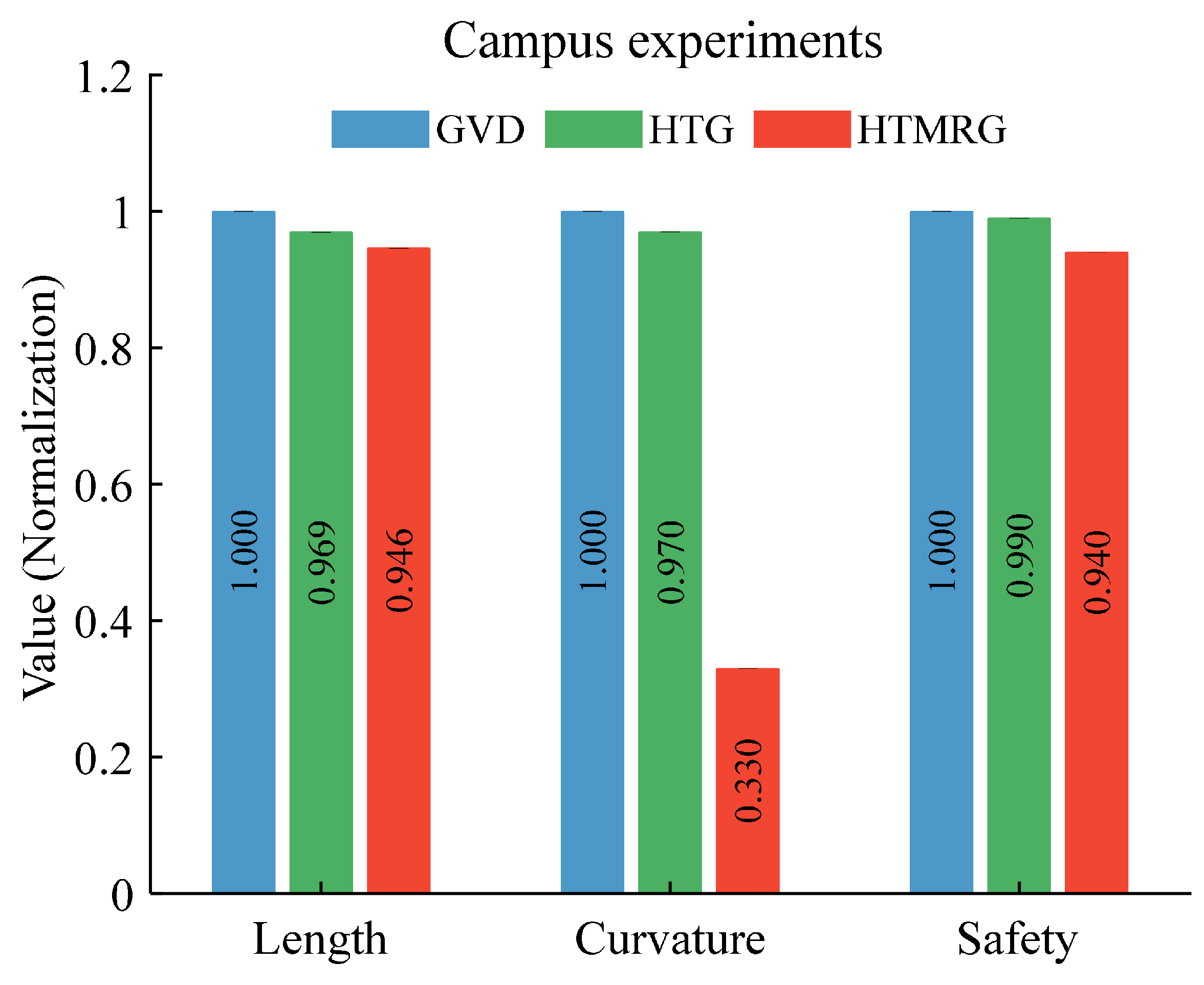
In addition, three representative autonomous navigation cases are illustrated in Figure 23. The yellow points correspond to LiDAR point clouds, which are visualized to indicate the vehicle’s position in the environment, while the vehicle pose is estimated through the localization module. The red line shows the smooth path generated by HTMRG-based planning, whereas the green line represents the path produced by HTG-based planning, which contains more abrupt turns. The red paths are tracked using an enhanced pure pursuit algorithm, based on our previous research [31]. Figure 24 presents a performance comparison of 50 planning cases with different start–goal pairs. The paths planned on HTMRG are shorter and smoother than those generated by SG and HTG, with only minimal compromise on safety.
Figure 23.
Path planning examples comparing HTG and HTMRG in a real-world campus environment. (a) Case 1. (b) Case 2. (c) Case 3.
Figure 24.
Performance comparison of different graphs representations in campus.
7. Conclusions and Outlook
In this study, we investigated a novel RG modeling method and its application to autonomous path planning. The proposed HTMRG framework reduces graph complexity, identifies intersections, and constructs SCEs and SIEs to generate high-quality road-network representations. To further enhance practical applicability, a dedicated start–goal insertion strategy was introduced for efficient path planning on HTMRG. Quantitatively, the proposed insertion strategy reduces the planned path length by 4.13–6.99% compared with the traditional insertion method. In addition, the hierarchical graph representation significantly accelerates graph search, achieving orders-of-magnitude speedup over Grid-based planning and an order-of-magnitude improvement over GVD-based planning. The framework also exhibits high reliability, where reliability refers to the success rate of generating feasible, collision-free paths across repeated start–goal trials.
Despite the promising results, several limitations remain. The current framework assumes a static environment and does not explicitly handle dynamic obstacles. In addition, the proposed method focuses on single-robot navigation and has not yet been extended to multi-UGV coordination scenarios. Furthermore, the road graph is constructed from prior maps and does not currently support fully online map generation and updating.
Future work will address these limitations by integrating dynamic obstacle avoidance mechanisms and incorporating model predictive control (MPC) for improved motion execution. We also plan to extend the HTMRG framework to multi-robot cooperative navigation and investigate online road-graph construction for continuously evolving environments.
Author Contributions
Conceptualization, S.Z. and X.X.; methodology, S.Z.; software, S.Z. and N.L.; validation, X.X. and T.Z.; formal analysis, S.Z.; investigation, S.Z.; resources, X.X. and S.Z.; data curation, S.Z.; writing—original draft preparation, S.Z.; writing—review and editing, S.Z.; supervision, X.X. All authors have read and agreed to the published version of the manuscript.
Funding
This work was supported in part by the Science Fund for Creative Research Groups of the National Natural Science Foundation of China (Grant No. 61921004), the Research Fund for Advanced Ocean Institute of Southeast University, Nantong (Key Program: KP202403) and Guangdong Basic and Applied Basic Research Foundation (Grant No. 2024A1515010269), the China Postdoctoral Science Foundation (Grant No. GZC20251181).
Data Availability Statement
The original contributions presented in this study are included in the article. Further inquiries can be directed to the corresponding author.
Conflicts of Interest
The authors declare no conflict of interest.
References
- Guo, Z.; Xia, Y.; Liu, J.; Gao, J.; Wan, P.; Xu, K. Path Planning Design and Experiment for a Recirculating Aquaculture AGV Based on Hybrid NRBO-ACO with Dueling DQN. Drones 2025, 9, 476. [Google Scholar] [CrossRef] [Scilit]
- Shao, J.; Cheng, J.; Xia, B.; Yang, K.; Wei, H. A Novel Service System for Long-Distance Drone Delivery Using the “Ant Colony + A*” Algorithm. IEEE Syst. J. 2020, 15, 3348–3359. [Google Scholar] [CrossRef] [Scilit]
- Wang, X.; Li, H.; Hu, M.; Dou, Q.; Ouyang, W.; Ma, G.; Li, Y.; Qin, H. HD Map Construction and Update System for Autonomous Driving in Open-Pit Mines. IEEE Syst. J. 2023, 17, 6202–6213. [Google Scholar] [CrossRef] [Scilit]
- Toda, Y.; Kubota, N. Path Planning Using Multi-Resolution Map for a Mobile Robot. In Proceedings of the SICE Annual Conference 2011, Tokyo, Japan, 13–18 September 2011; IEEE: New York, NY, USA, 2011; pp. 1276–1281. [Google Scholar]
- Barber, R.; Crespo, J.; Gómez, C.; Hernández, A.C.; Galli, M. Mobile Robot Navigation in Indoor Environments: Geometric, Topological, and Semantic Navigation; IntechOpen: London, UK, 2018. [Google Scholar]
- Zhang, J.; Xia, Y.; Shen, G. A Novel Learning-Based Global Path Planning Algorithm for Planetary Rovers. Neurocomputing 2019, 361, 69–76. [Google Scholar] [CrossRef] [Scilit]
- Gao, G.; Lu, J.; Guan, W. CE-Bi-RRT*: Enhanced Bidirectional RRT* with Cooperative Expansion Strategy for Autonomous Drone Navigation. Drones 2025, 9, 831. [Google Scholar] [CrossRef] [Scilit]
- Zhang, C.; Wang, G.; Chen, M.; Lin, Y.; Li, K.; Wu, M.; Li, Z.; Wang, Q. E-Planner: An Efficient Path Planner on a Visibility Graph in Unknown Environments. IEEE Trans. Instrum. Meas. 2024, 73, 8506214. [Google Scholar] [CrossRef] [Scilit]
- Nguyet, T.T.N.; Van Hoai, T.; Thi, N.A. Some Advanced Techniques in Reducing Time for Path Planning Based on Visibility Graph. In Proceedings of the 2011 Third International Conference on Knowledge and Systems Engineering, Hanoi, Vietnam, 14–17 October 2011; IEEE: New York, NY, USA, 2011; pp. 190–194. [Google Scholar]
- Zhou, S.; Xu, X.; Zhong, M. A Path Planning Method Based on Simplified Visibility Graph and Support Vector Machine. In Proceedings of the 2023 8th International Conference on Automation, Control and Robotics Engineering (CACRE), Hong Kong, China, 13–15 July 2023; IEEE: New York, NY, USA, 2023; pp. 236–241. [Google Scholar]
- Jin, Q.; Hu, Q.; Zhao, P.; Wang, S.; Ai, M. An Improved Probabilistic Roadmap Planning Method for Safe Indoor Flights of Unmanned Aerial Vehicles. Drones 2023, 7, 92. [Google Scholar] [CrossRef] [Scilit]
- Liu, R.; Wang, J.; Zhang, B. High Definition Map for Automated Driving: Overview and Analysis. J. Navig. 2020, 73, 324–341. [Google Scholar] [CrossRef] [Scilit]
- da Silva, J.A.R.; Gomes, I.P.; Wolf, D.F.; Grassi, V. Sparse Road Network Model for Autonomous Navigation Using Clothoids. IEEE Trans. Intell. Transp. Syst. 2020, 23, 885–898. [Google Scholar] [CrossRef] [Scilit]
- Mi, X.; Yang, B.; Dong, Z.; Chen, C.; Gu, J. Automated 3D Road Boundary Extraction and Vectorization Using MLS Point Clouds. IEEE Trans. Intell. Transp. Syst. 2021, 23, 5287–5297. [Google Scholar] [CrossRef] [Scilit]
- Zhang, Z.; Li, J.; Guo, Y.; Yang, C.; Wang, C. 3D Highway Curve Reconstruction from Mobile Laser Scanning Point Clouds. IEEE Trans. Intell. Transp. Syst. 2019, 21, 4762–4772. [Google Scholar] [CrossRef] [Scilit]
- Kwon, T.-B.; Song, J.-B. Real-Time Building of a Thinning-Based Topological Map. Intel. Serv. Robot. 2008, 1, 211–220. [Google Scholar] [CrossRef] [Scilit]
- Stenzel, J.; Lünsch, D.; Schmitz, L. Automated Topology Creation for Global Path Planning of Large AGV Fleets. In Proceedings of the 2021 IEEE International Intelligent Transportation Systems Conference (ITSC), Indianapolis, IN, USA, 19–22 September 2021; IEEE: New York, NY, USA, 2021; pp. 3373–3380. [Google Scholar]
- Sandström, R.; Uwacu, D.; Denny, J.; Amato, N.M. Topology-Guided Roadmap Construction with Dynamic Region Sampling. IEEE Robot. Autom. Lett. 2020, 5, 6161–6168. [Google Scholar] [CrossRef] [Scilit]
- Lien, J.-M.; Thomas, S.L.; Amato, N.M. A General Framework for Sampling on the Medial Axis of the Free Space. In Proceedings of the 2003 IEEE International Conference on Robotics and Automation (Cat. No. 03CH37422), Taipei, Taiwan, 14–19 September 2003; IEEE: New York, NY, USA, 2003; pp. 4439–4444. [Google Scholar]
- Telli, S.; Menebröker, F.; Stenzel, J. Spline-Based Topology Generation for Path Planning of Mobile Robots under Kinematic Constraints. In Proceedings of the 2023 5th International Conference on Control and Robotics (ICCR), Tokyo, Japan, 23–25 November 2023; IEEE: New York, NY, USA, 2023; pp. 130–139. [Google Scholar]
- Noël, T.; Lehuger, A.; Marchand, E.; Chaumette, F. Skeleton Disk-Graph Roadmap: A Sparse Deterministic Roadmap for Safe 2D Navigation and Exploration. IEEE Robot. Automat. Lett. 2023, 9, 555–562. [Google Scholar] [CrossRef] [Scilit]
- Han, J.-W.; Jeon, S.; Kwon, H.J. Hierarchical Topology Map with Explicit Corridor for Global Path Planning of Mobile Robots. Intel. Serv. Robot. 2023, 16, 195–212. [Google Scholar] [CrossRef] [Scilit]
- Li, N.; Yao, Y.; Xu, X.; Peng, Y.; Wang, Z.; Wei, H. An Efficient LiDAR SLAM with Angle-Based Feature Extraction and Voxel-Based Fixed-Lag Smoothing. IEEE Trans. Instrum. Meas. 2024, 73, 8506513. [Google Scholar] [CrossRef] [Scilit]
- Abou Merhy, B.; Payeur, P.; Petriu, E.M. Application of Segmented 2-D Probabilistic Occupancy Maps for Robot Sensing and Navigation. IEEE Trans. Instrum. Meas. 2008, 57, 2827–2837. [Google Scholar] [CrossRef] [Scilit]
- Fredriksson, S.; Saradagi, A.; Nikolakopoulos, G. GRID-FAST: A Grid-based Intersection Detection for Fast Semantic Topometric Mapping. J. Intell. Robot. Syst. 2024, 110, 154. [Google Scholar] [CrossRef] [Scilit]
- Bertolazzi, E.; Frego, M. G1 Fitting with Clothoids. Math. Methods Appl. Sci. 2015, 38, 881–897. [Google Scholar] [CrossRef] [Scilit]
- Lee, J.-T.; Kang, T.-W.; Choi, Y.-S.; Jung, J.-W. Clearance-Based Performance-Efficient Path Planning Using Generalized Voronoi Diagram. Int. J. Fuzzy Logic Intell. Syst. 2023, 23, 259–269. [Google Scholar] [CrossRef] [Scilit]
- Hou, Q.; Zhang, S.; Chen, S.; Nan, Z.; Zheng, N. Straight Skeleton Based Automatic Generation of Hierarchical Topological Map in Indoor Environment. In Proceedings of the 2021 IEEE International Intelligent Transportation Systems Conference (ITSC), Indianapolis, IN, USA, 19–22 September 2021; IEEE: New York, NY, USA, 2021; pp. 2229–2236. [Google Scholar]
- Shan, T.; Englot, B.; Meyers, D.; Wang, W.; Ratti, C.; Rus, D. LIO-SAM: Tightly-Coupled LiDAR Inertial Odometry via Smoothing and Mapping. In Proceedings of the 2020 IEEE/RSJ International Conference on Intelligent Robots and Systems (IROS), Las Vegas, NV, USA, 24 October 2020–24 January 2021; IEEE: New York, NY, USA, 2020; pp. 5135–5142. [Google Scholar]
- HViktorTsoi. A Simple Localization Framework That Can Re-localize in Built Maps Based on FAST-LIO. Available online: https://github.com/HViktorTsoi/FAST_LIO_LOCALIZATION (accessed on 11 January 2026).
- Chi, C.; Xu, X.; Zhou, S.; Wang, Y. Adaptive Control of Path Tracking Based on Improved Pure Pursuit Algorithm. In Proceedings of the 3rd International Conference on Autonomous Unmanned Systems, Nanjing, China, 8–11 September 2023; Springer: Berlin/Heidelberg, Germany, 2023; pp. 56–65. [Google Scholar]

Disclaimer/Publisher’s Note: The statements, opinions and data contained in all publications are solely those of the individual author(s) and contributor(s) and not of MDPI and/or the editor(s). MDPI and/or the editor(s) disclaim responsibility for any injury to people or property resulting from any ideas, methods, instructions or products referred to in the content. |
© 2026 by the authors. Licensee MDPI, Basel, Switzerland. This article is an open access article distributed under the terms and conditions of the Creative Commons Attribution (CC BY) license.