MuRDE-FPN: Precise UAV Localization Using Enhanced Feature Pyramid Network

Highlights

What are the main findings?

• We propose MuRDE-FPN, an end-to-end cross-view drone localization method based on a one-stream transformer-based (OS-PCPVT) backbone. To improve the positioning, our decoder includes two novel modules: a multi-receptive deformable enhancement (MuRDE) block to enhance the most semantically rich feature layer and a feature alignment module (FAM) that accounts for spatial misalignment between feature maps.
• The proposed method improves localization accuracy compared with similar methods. A performance increase is noted on both standard and more challenging datasets.

What are the implications of the main findings?

• Our method effectively localizes UAVs in both urban and mixed environments. Moreover, MuRDE-FPN works in both low- and high-altitude settings.
• Given a negligible increase in the computational load, the proposed method can be deployed efficiently in resource-constrained environments.

Abstract

Unmanned aerial vehicles (UAVs) require reliable autonomous positioning independent of external satellite navigation signals, motivating the development of a vision-based, end-to-end finding point in map (FPI) framework. This study introduces MuRDE-FPN, an enhanced feature pyramid network (FPN) designed for precise UAV localization, building upon a lightweight one-stream transformer-based (OS-PCPVT) backbone. MuRDE-FPN integrates efficient channel attention (ECA) for adaptive channel recalibration and features two novel components: a multi-receptive deformable enhancement (MuRDE) that utilizes deformable convolutions with varying kernel sizes to refine the semantically rich final feature layer, and a feature alignment module (FAM) for cross-level fusion. Evaluated on the UL14 dataset and a new, more diverse UAV-Sat dataset, MuRDE-FPN consistently outperformed four state-of-the-art FPI methods (FPI, WAMF-FPI, OS-FPI, DCD-FPI). It achieved a relative distance score of 84.26 on UL14 and 63.74 on UAV-Sat datasets, demonstrating improved localization. Ablation studies confirmed the cumulative benefits of ECA, MuRDE, and FAM. These findings highlight the effectiveness of custom FPN designs and targeted feature enhancements for precise cross-view positioning, with MuRDE-FPN providing a robust solution and the UAV-Sat dataset offering a new benchmark for evaluation. Future efforts will address computational efficiency and performance across varying data quality environments.

1. Introduction

In recent years, unmanned aerial vehicles (UAVs) have surged in popularity and in the scope of their applications. While UAVs have been previously used in the military domain, the use of drones in the civilian sector is also booming. Drones are frequently used in agriculture [1], safety and emergency missions [2], and logistics [3]. Integrating UAVs with reliable autonomous decision making is crucial for reducing time and resource costs.

To accurately position a UAV, the current technology relies on global navigation satellite system (GNSS) sensors. This, however, is not reliable in all scenarios, as global positioning system (GPS) signals are susceptible to natural interference, spoofing, and jamming. To put it simply, there is a need for autonomous positioning technology that is not based on irregular sensor data. In GNSS-challenged settings, a standard self-contained solution is the inertial navigation system (INS), typically implemented as a strapdown inertial navigation system (SINS), which integrates inertial measurement unit data to estimate attitude, velocity, and position. In practice, however, stand-alone INS/SINS suffers from error accumulation (so called drift) over time due to sensor biases and noise [4] and therefore is commonly aided by an external source or information (e.g., GNSS, vision, LiDAR, map/terrain constraints) to reduce the accumulated error. Similarly, LiDAR-based mapping approaches, while more accurate, introduce additional constraints due to increased equipment and computational requirements. These issues motivate the exploration of vision-based algorithms either as a substitute or a supplement to such methods.

With the rise of computer vision (CV) algorithms and the availability of remote sensing imagery, vision-based methods have been employed to position a UAV in a satellite. In this context, estimating the drones’ position can be achieved using handcrafted feature-matching approaches. These methods are the basis of many vision simultaneous localization and mapping (SLAM) pipelines; however, they suffer from poor robustness when viewpoint, illumination, and scale changes. For instance, scale-invariant feature transform [5], frequently used in vision SLAM to find and match keypoints within images, is notorious for degraded performance under noise, viewpoint and light changes [6]. Some matching-based approaches integrate deep learning (DL) into their pipeline. For instance, ref. [7] proposed using a convolutional neural network (CNN) to extract local descriptors and match them using a graph neural network. Finally, ref. [8] used a custom CNN when extracting global features, thus enhancing key-point matching with fused local and global features. However, while these approaches are computationally cheap and fast, they still suffer from poor robustness when viewpoint, illumination, and scale variations are present.

Due to advancements in CV, different detector-free localization approaches have been proposed. Currently, there are two main ways to position a drone using DL pipelines: either retrieve the most similar satellite patch from a satellite image gallery or precisely locate the point within a satellite image. While satellite retrieval was the predominant CV-based approach [9,10,11], it suffers some drawbacks. First, to achieve localization via the retrieval method onboard, additional preprocessing and disk space is required. Every patch of the satellite image must have its features extracted, which increases the computational cost during deployment. Then, similarities for the current view and all of the images in the constructed satellite gallery need to be calculated every time the position needs to be estimated. Moreover, the computational load of such procedures scales up with the size of the satellite map.

In recent years, Dai et al. [12] proposed an end-to-end precision localization framework referred to as finding point in map (FPI). The FPI approach aims to solve some of the problems of the satellite retrieval method. In particular, it aims to reduce heavy data preprocessing, memory cost, and improve precise positioning by locating the UAV within the satellite map directly and producing a dense heatmap of possible locations. Recently, Chen et al. [13] proposed a one-stream model that drastically reduced model computational complexity. Since then, research in FPI has shifted from using two-stream methods that are Siamese-like to one-stream backbone extractors and restoring the original output resolution with various decoding strategies. Overall, in FPI, a lot of work has been done in designing better, more lightweight one-stream feature extractors [13,14,15,16], as this is where critical advancements in lowering computational cost can be achieved. In this context, the decoding strategy should not be overlooked, as it has been shown that different decoding designs are crucial to overall performance as well. However, the specific decoding strategies usually rely on the particular architecture of the backbone, as some of them do cross-modal modeling in every stage [13,14], and others only at the lower levels [15,16]. Rather than proposing a new backbone architecture, we suggest adopting the most widely used [13,17] one-stream pyramid vision transformer with conditional positional encoding (OS-PCPVT) as a strong baseline. In recent years, the literature on dense prediction tasks has shifted towards enhancing standard feature pyramid network (FPN)-based decoders towards more task-suitable FPN designs. We believe in the potential of custom FPN refining methods, with special focus on certain scales, particularly for precise UAV localization in challenging, real-world environments.

In any DL framework, the scope of generalizability matters as much as the whole method. This makes training and validation data of great importance and, as of this day, there is only one dataset that is used throughout all FPI research—UL14 [12]. In other words, only one benchmark dataset exists, as FPI in itself is a relatively new task, and traditional UAV–satellite pair datasets are insufficient. This hinders the comparison and evaluation of different methodologies, as, while the dataset itself is properly constructed, it has its own limitations. The main problem with UL14 is that the data are very homogenous. This property holds true for both the content (similar architecture and areas) and quality (UAV flights were conducted at a low height; satellite imagery showed little to no change). For this reason, evaluating methods on this dataset alone is not sufficient in conducting more rigorous comparisons of methods and extending the findings to a more natural setting. While there is some research that extends the analysis beyond UL14 [14,15,16,18,19], the comparative datasets are not as rigorous as the UL14, because in those studies only one satellite search map is used [18], the impact of satellite size on UL14 is not reported [14], or the satellite map is insufficient to extend precision positioning findings towards bigger satellite maps [15,16,18].

In summary, despite recent progress in FPI-based UAV localization, several gaps remain. First, most existing works primarily focus on backbone architecture design, while decoder structures, while frequently customized, rarely employ level-aware strategies that explicitly account for the complementary semantic richness of deeper feature layers and the spatial accuracy of the shallower ones. Second, evaluation is overwhelmingly centered on the UL14 dataset, which, while well-constructed, exhibits limited content diversity and relatively small satellite search areas. Third, the behavior of FPI methods under large-area, high-altitude localization scenarios remains under-explored, even though such conditions are common in real-world UAV operations. This work explicitly targets these three gaps. Seeking to enrich the scientific literature in UAV localization, our key contributions can be summarized as follows:

• Seeking to emulate the difficulty and benchmarking characteristics of the UL14 dataset, we developed a novel UAV–satellite pair dataset for extended FPI task analysis. Our dataset, UAV-Sat, retains the quality of different satellite size imagery in the test set, yet the content of the dataset is more general purpose and representative of diverse UAV applications.
• Development of a lightweight transformer-based network featuring a novel FPN design that incorporates multi-receptive deformable convolutions to enhance the final backbone feature layer, along with feature alignment between high- and mid-level feature maps.
• Extensive comparative analysis of our method on two datasets (UL14, UAV-Sat) and an exhaustive ablation study of our method.

2. Related Work

2.1. Transformer-Based Computer Vision Architectures

The transformer architecture was first introduced by Vaswani et al. [20] and has been widely used ever since. While originally created for natural language processing tasks, transformer-based DL architectures have been widely used in CV. Generally, any transformer-based DL method relies on an attention mechanism that works as follows: Given an input sequence, three sets of vectors—queries, keys, and values—are generated through learnable linear projections. For every query vector, an attention weight is computed by calculating the dot product between it and all key vectors and normalizing with the softmax function. These weights reflect the relative importance of different input elements. The final output is obtained as a weighted sum of the value vectors, and in this way, the most informative parts of the input are focused on the most. Unlike convolutional operations, which have a fixed receptive field, the previously described attention mechanism allows for long-range modeling, as queries, keys, and values interact across the entire input sequence, regardless of spatial distance.

With the introduction of the first vision transformer (ViT) [21], transformer-based architectures were successfully integrated into the field of vision processing. In ViT, images are divided into patches, then those patches are processed in a transformer encoder using self-attention, just like sequences of text tokens would be processed. While such simple techniques enabled transformer-based architectures to be used in CV, ViT was limited in its applicability, as it was tailored for image classification. However, since then, various transformer-based architectures have been developed, each better suited to general purpose CV tasks than the original ViT and, in many cases, competitive or superior to their CNN counterparts.

For instance, Wang et al. [22] proposed a more task-flexible pyramid vision transformer (PVT). Notably, PVT has a hierarchical feature structure, which was made possible by progressively strided patch embedding layers. Given that transformer-based architectures are costly in terms of memory and computational resources, PVT additionally introduced spatial reduction attention, which reduced resource costs while still achieving strong performance. Another hierarchical vision transformer, Swin [23], lowered the computational complexity by replacing global attention with window-based attention. Window-based attention is a variant of attention, where communication between tokens is restricted within fixed-size windows, and this, in turn, lowers computational complexity requirements. Swin specifically does not use global attention and instead captures long-range dependencies gradually across layers by shifting the window partitioning in each consecutive layer. Chu et al. [24] introduced Twins-PCPVT, a PVT with conditional positional encoding (CPE) in every stage after the transformer encoder layer. In simplified terms, CPE encodes positional information by using depth-wise convolutions to retain spatial relationships between features. Just like Swin, Twins-PCPVT used window-attention; instead of shifting the windows to capture global dependencies, the communication between windows was achieved by using spatially sub-sampled representative tokens. The second version of PVT was introduced [25], where overlapping patch embedding was used, and spatial reduction attention was further improved. Since the introduction of these and subsequent models, transformer-based architectures have been able to perform efficient, multi-scale feature extraction and incorporate transformers into dense prediction tasks.

With transformers, it is also possible to model cross-feature—and by extension cross-image—interactions. A type of attention, referred to as cross-attention, operates by sampling queries from one, and keys/values from another feature representation. Cross-attention and its variants have been used in cases where cross-modality interaction is inherent to the task, such as image-to-image matching or multi-view perception. For instance, both Matchformer [26] and LoFTR [27] employ self- and cross-attention to explicitly match features within and between image pairs and thus enabling robust correspondence estimation. Likewise, OSTrack [28] applies the same principle of using both attention mechanisms to create a one-stream framework between template and search images for object tracking. These examples demonstrate that transformer-based algorithms are effective in extending their usability not only for feature extraction but also for modeling early and task-specific feature interactions across multiple inputs.

2.2. Feature Pyramid Networks

FPNs as a specific design choice have been used in a variety of cases. As a modeling structure, FPNs are used when a task needs strong performance across scales or when a task requires pixel-level performance (as in segmentation or depth estimation). First feature pyramid network [29] was proposed to mitigate the natural loss of spatial details when using modern CNN-based (and more recently, transformer-based) vision models. A typical FPN exploits multi-scale feature representations and constructs such feature representation that preserves semantic richness and spatial resolution and is suitable for subsequent downstream tasks.

The core idea behind any FPN is as follows: Instead of using the last and most spatially compressed feature layer, the integration of previous feature maps should not be overlooked. For instance, in the seminal FPN [29] work, it is suggested to construct FPN in the following way: Given the hierarchical nature of any backbone network, feature maps from different levels are combined with a top-down pathway using lateral connections. In them, higher level features are progressively upsampled and merged (in [29], a simple addition operation is sufficient for a merge) with lower level (and higher resolution) ones. In recent years, FPNs have evolved significantly, with main differences in architectural design being those of the pyramid topology and micro-architectural design choices (such as using different feature upsampling, refinement, and merging logic).

For instance, Liu et al. [30] introduced PANet—an FPN with an additional bottom-up path, adaptive feature pooling, and fully connected fusion. Later, NAS-FPN [31] introduced dynamic FPN topology search; instead, of using a predetermined architecture design, NAS-FPN used a controller network to generate FPN architecture dynamically. In essence, to get the optimal design, a recurrent neural network was trained—its input was sampled from candidate FPN architectures (for instance, feature level selection, merging operation) and its reward was defined as the selected architecture’s performance on the validation set. While such a method resulted in an improved performance compared with hand-crafted FPNs at the time, it also incurred higher computational complexity. Later, Tan et al. [32] introduced BiFPN—a bidirectional FPN that included various design choices. Just like the PANet, it includes a bottom-up path, but like NAS-FPN, the blocks of top-down are repeated. Nodes with a single input are removed, and features are fused with learnable fusion.

FPN architectures can sometimes be designed asymmetrically, as, in certain cases, there is prior knowledge that selectively enhancing specific feature levels can be more beneficial than uniform processing. For instance, to improve the semantic segmentation of maritime images, Sun et al. [33] used an information interaction module that explicitly integrates raw images with high-level feature representations (in this case, the last two layers). These three inputs are jointly processed, and a new feature map is generated, which is integrated into the top-down FPN pathway. Xie et al. [34] also used a highly asymmetric decoder (top-down FPN path) structure with multiple architectural enhancements for better image segmentation. First, instead of the usual channel unification with typical convolution with kernel size 1, squeeze and excitation blocks were used to adaptively reweight the channels. Second, the global semantic branch processed inputs from the last two feature extractor layers [34].

In certain circumstances, it is not unusual to find improvements not only in FPN topology but also in the introduction of task-specific FPN enhancements. For example, in medical image segmentation, retaining or extracting boundary information is key to improving performance. This reasoning is why Thuan et al. and Zhang et al. [35,36] both used the reverse attention mechanism—a technique that controls how information flows and can specifically help enhance edge information—in their decoder (top-down) paths. Another example of extending pyramid structures in enriching feature representations for the task at hand is provided by Zhou et al. [37]. In their work, the authors tackle small object detection, and, to enhance feature richness, ref. [37] employs multi-receptive field-based enhancement modules. Interestingly, these modules are used only on specific feature maps (the first two least spatially reduced ones), which again showcases an asymmetric FPN modeling. Such findings in a broader context imply that task-specific FPN design choices, especially those that extend FPN beyond topology, are of great importance to overall model effectiveness.

2.3. Finding Point in Map

To enable more precise UAV localization, Dai et al. [12] proposed an end-to-end dense prediction approach. First, the authors outlined two relevant metrics—relative distance score (RDS) and meter-level accuracy—and formulated UAV localization as a dense prediction task, FPI. In FPI, the final output of a model should be a satellite-sized grid of probabilities that notes whether a point on the map is a central UAV location. To achieve such an output, two backbones of DeiT-S [38] (backbone for UAV and satellite) are used as feature extractors, then the interaction between these features is calculated using Siamese cross-correlation. The authors additionally implement a true positive generation technique to balance low true positive cases; instead of treating only one point as the only possible true positive, they sample an area around ground truth (creating a synthetic true positive grid). Then, weighted balance loss is used to additionally counteract the imbalanced nature of this task.

Following the FPI approach, Wang et al. [39] proposed a weight-adaptive multi-feature fusion (WAMF-FPI) method: a two-stream network with PCPVT-S [24] as a backbone feature extractor, feature pyramid neck, and weighted fusion. The WAMF-FPI method differs from the original FPI method in that it uses a hierarchical vision transformer to extract features at different levels, as opposed to just using the last layer, where features are semantically rich but also lose their positional information. Additionally, cross-correlations between UAV features and last satellite feature maps are calculated, and weighted fusion is used. According to Wang et al. [39], these techniques enable to prevent spatial information loss, which was prevalent in the original FPI approach. Moreover, the authors propose a new loss weighing method—Hanning loss—where true positives are weighed according to their distance to the central point. This allows models to focus more on the central area rather than treating all true positive points the same. WAMF-FPI outperformed the original FPI approach on the UL14 dataset.

Chen et al. [13] proposed a one-stream feature extractor, OS-PCPVT, that leveraged both self- and cross-attention to capture early feature interactions. Using such a backbone design greatly reduced model size, which is especially relevant when regarding onboard deployment. The authors additionally used atrous convolution after feature extraction to capture relevant pixel-level information and improve restoration. Most notably, in [13] multi-task training is employed to predict not only the final heatmap but also an additional offset for vertical and horizontal directions. For this reason, a combined loss function was used, where classification was evaluated using Hanning loss, and smooth L2 loss was used for the regression task. Similarly, He et al. [17] leveraged the OS-PCPVT backbone, with emphasis on fusing features across different stages. Instead of using standard FPN, in [17] adaptive spatial feature fusion was included, and spatial weights were generated for each feature map. Additionally, a custom head was used to achieve optimal spatial restoration; it contained a key module composed of deformable convolutions that progressively reduced the channel count and increased the spatial dimension.

The latest research in FPI involves the work of Fan et al. [15], who proposed their own single-stream pyramid transformer (SSPT) model that, like OS-PCPVT, is one-stream and hierarchical. Notably, SSPT does not employ cross-attention at every stage, it is applied only at the final one. Crucially, the allocation of self-attention in the first two backbone stages and cross-attention in the last stage yields the best results. Then, the final heatmap is also restored from only that same last feature layer. To avoid positional loss, progressive upsampling and a multi-scale pyramid design were used. Notably, the authors also propose using Gauss loss, which is similar to Hanning loss except that the weighting is performed with the Gaussian window function. Expanding upon SSPT, Ju et al. [16] included a channel-reduction attention mechanism in the backbone and designed a residual feature pyramid network, and Chen et al. [14] combined both self- and cross-attention at every feature extraction stage with a symmetrical feature pyramid network, allowing for adequate incorporation of the most semantically rich feature layer. A slightly different approach was proposed by Tian et al. [18]: instead of using a traditional vision transformer, the authors incorporated vision Mamba to capture long range dependencies. Additionally, the authors used consistency regularization training with center masking augmentation so that the model would learn to predict the output even when central UAV features are missing.

To sum up, prior FPI methods moved from single-layer decoding towards multi-scale feature aggregation to mitigate spatial information loss. In FPI, the deepest feature layer carries the most discriminative cross-view semantics but is also the most affected by spatial downsampling. This motivates selectively refining only the deepest semantic feature layer rather than uniformly enhancing all scales. Furthermore, FPI requires precise spatial correspondence between UAV and satellite features across scales. Given that misalignment during feature extraction can degrade the final performance, it seems fruitful to explore cross-scale feature fusion methods beyond conventional strategies.

3. Materials, Method and Evaluation

3.1. Datasets and Preprocessing

To evaluate our method, we utilized two publicly available UAV–satellite pair datasets: UL14 [12] and UAV-VisLoc [40]. The UL14 dataset was left as is; however, from UAV-VisLoc, we created our own, UAV-Sat dataset. While UL14 is crucial for evaluation as a benchmark dataset for the FPI task, the addition of UAV-Sat allows to extend our findings to a setting in which satellite maps are comparatively larger and more variable and the UAV images are sampled from a higher altitude. In the following subsections, we outline the specifics of each dataset and our data preprocessing configuration. Both the UL14 and UAV-Sat datasets were created so that the validation and test sets include augmented images. This makes the method’s validation much more reliable.

3.1.1. UL14 Dataset

UL14 consists of UAV–satellite image pairs from 14 different university campuses in China, 10 of which are for training and 4 for testing. The training set comprises UAV images at 512 × 512 pixels, and satellite images at 1280 × 1280 pixels. The test set contains UAV images at 256 × 256 pixels, and satellite images at 768 × 768 pixels. The satellite imagery in this dataset has a spatial resolution of 0.294 m/pix. Unprocessed training set satellite imagery is centrally aligned, meaning that the UAV is at the center of the paired satellite patch. Satellite images from the test set, however, do not share this quality; they are not centrally aligned and also have varying sampling scales. In the test set, for each UAV image there are 12 satellite patch images, in which the UAV location is randomly distributed, and satellite scales vary from 700 to 1800 pixels.

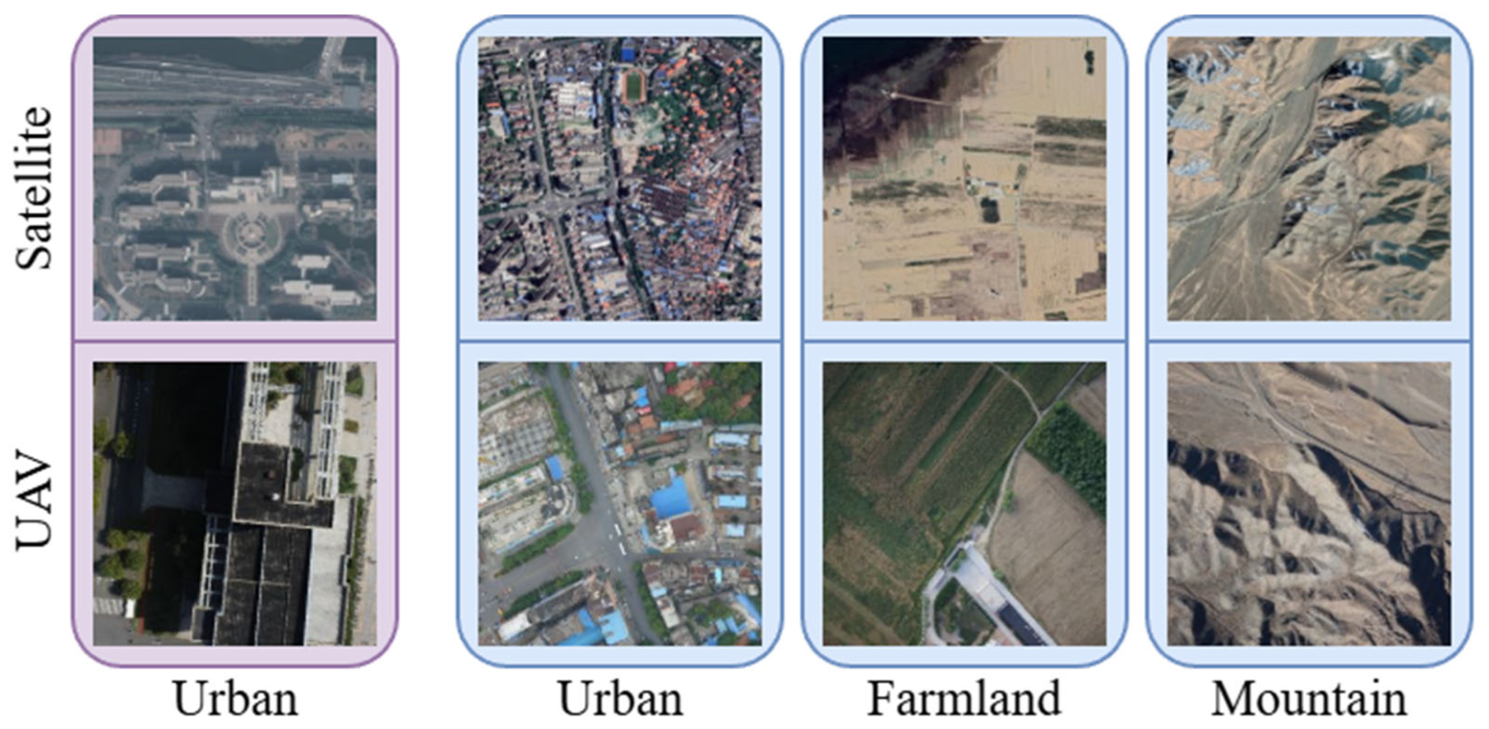
UAV images are sampled from 80, 90, or 100 m heights, which makes this dataset low altitude in terms of UAV data. Most satellite images in UL14 exhibit a relatively straight-down view, with little visible tilt. Qualitatively, since UAV images are sampled from university campuses, this dataset is urban-focused, with no suburban areas or challenging nature environments (such as deserts, valleys, mountains). Together with the absence of any noticeable off-nadir satellite imagery, UL14 is a relatively limited dataset for general purpose UAV positioning applications.

3.1.2. The Creation of UAV-Sat Dataset

To evaluate and enhance the applicability of our method and to address the limitations of the UL14 dataset, from the publicly available UAV-VisLoc dataset we created our own UAV-Sat dataset that aligns with the objectives of the FPI task. Originally, UAV-VisLoc comprised UAV–satellite image pairs and was collected from 9 various regions in China. Differing from UL14, this dataset is more diverse in terms of visual content: UAV-VisLoc contains images from both manmade (urban and suburban) and natural (river valleys, farmlands, mountainous areas) environments. UAV flight heights range from 405 to 840 m, making this dataset more applicable in evaluating the performance in high-altitude scenarios. Compared with the satellite imagery of UL14, UAV-VisLoc satellite images exhibit a greater amount of change because of the time difference between satellite and UAV capture. This makes UAV-VisLoc better suited for evaluating methods under realistic conditions in which satellite imagery may be suboptimal. The satellite imagery in this dataset has a spatial resolution of 0.3 m/pix. From UAV-VisLoc we created our own UAV-Sat dataset by using the following procedures:

• Inclusion of UAV–satellite pairs within the whole dataset: We chose to exclude pairs that contained UAV images with uninformative or non-pertinent features. For this purpose, UAV images were centered cropped, and if the images were deemed uninformative after this procedure, they were excluded from the final dataset. We consider an image to be informative if it contains some sort of permanent feature (e.g., a docking station on a shore, some road within the forest, permanent natural landmarks). We also excluded pairs with satellite images for which it was not possible to crop them to a 3500 × 3500 pixel range without padding.
• Train, validation, and test set splitting: After initial image selection, training, validation, and test sets were constructed, splitting the whole dataset into training and test sets (85/15 ratio) and then splitting the training set again into training and validation sets (90/10 ratio). Final splitting proportions were 76.5/8.5/15.
• Train set preparation: For the training set, we chose to crop satellite images to 3500 × 3500 pixels to get enough coverage area for random scale crop (RSC, see Section 3.1.2) augmentation and enrich the final dataset with bigger satellite coverage images. Such image cropping yields image pairs that cover approximately a 1 square kilometer satellite area. UAV images were not processed further (the same center crop from step 1 was retained).
• Validation and test set preparation: As in the training set, we also cropped satellite images to 3500 × 3500 pixels and retained the center crop of UAV from step 1. Additionally, each satellite image underwent RSC augmentation in a similar manner to the UL14 dataset. For every image, we constructed 12 satellite images of varying sizes, with the minimum satellite image size being 2400 pixels and the maximum being 3500 pixels. Notably, each of those 12 images had its target location pixel randomly sampled.
• Image format and saving: after the initial processing (steps 1–4) images were saved to a fixed resolution of 512 × 512 and 1280 × 1280 for UAV and satellite images, respectively, in the training set and 256 × 256 and 768 × 768 for UAV and satellite images, respectively, in the validation/training sets.

These steps were taken to ensure that our UAV-Sat dataset would be as comparable in evaluation difficulty to the UL14 as possible.

Table 1. Comparison between UL14 and UAV-Sat datasets. Sat and UAV denote the number of satellite and UAV images in the dataset.

	Dataset
	UL14			UAV-Sat (Ours)
	Sat	UAV	Satellite Cover Area *, km2	Sat	UAV	Satellite Cover Area *, km2
Train	6768	6768	0.1475	3330	3330	1.1025
Test	27,972	2331	0.0441–0.2916	7836	653	0.5184–1.1025

* The satellite area for the test set is a range of values, since in both datasets there are 12 satellite images of different scales.

and Figure 1 highlight a comparison between the two datasets.

3.1.3. Data Preprocessing

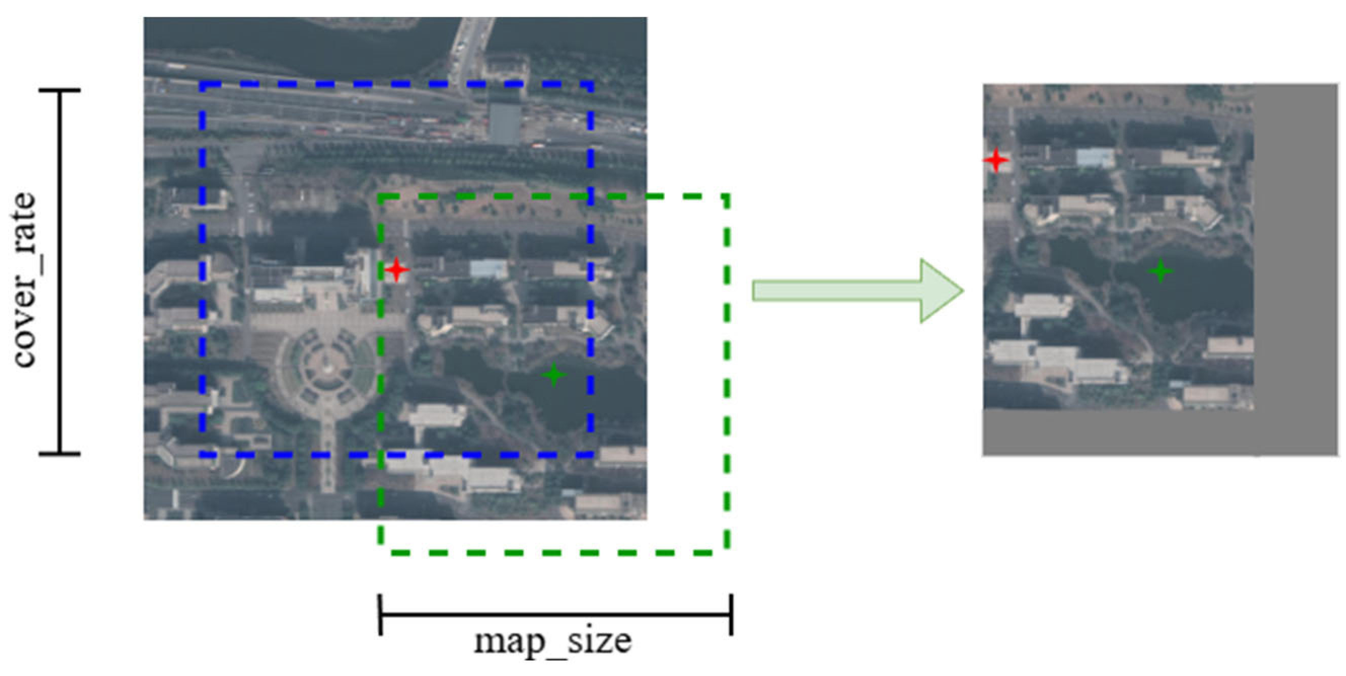
As previous studies have done, in the data preprocessing module we included RSC [12] (visualized in Figure 2). Given a centered image (i.e., an image where the target is at the center), this augmentation selects a random new point and crops a specific area around it. The coordinates of the true location are then recalculated, and the target location is no longer centered. Instead, it appears at a random location within the cropped area. This augmentation has two main parameters: map_size and cover_rate. The cover_rate parameter controls the range around the centered true location where a new random new point can be sampled, and the map_size controls how much of the area around the randomly sampled dot is covered.

In our case, this specific augmentation was used to expand both the training sets (RSC applied randomly with respect to the cover area) and the validation/test sets (the same augmentation applied statically, with the cover area fixed to a set of predefined sizes). By applying RSC in such a way, we ensure that there is no center bias during training and that our validation/test sets are more complex to classify, and thus our evaluation is more reliable.

Additionally, our data preprocessing pipeline includes an image normalization module, as we scale our images to be in the range of $\left[-1, 1\right]$. This type of normalization was selected since our initial experiments (conducted only on UL14) yielded superior performance compared with min-max scaling (value range $\left[0, 1\right]$). Such preprocessing was performed during the training, validation, and testing phases.

3.2. Backbone Network

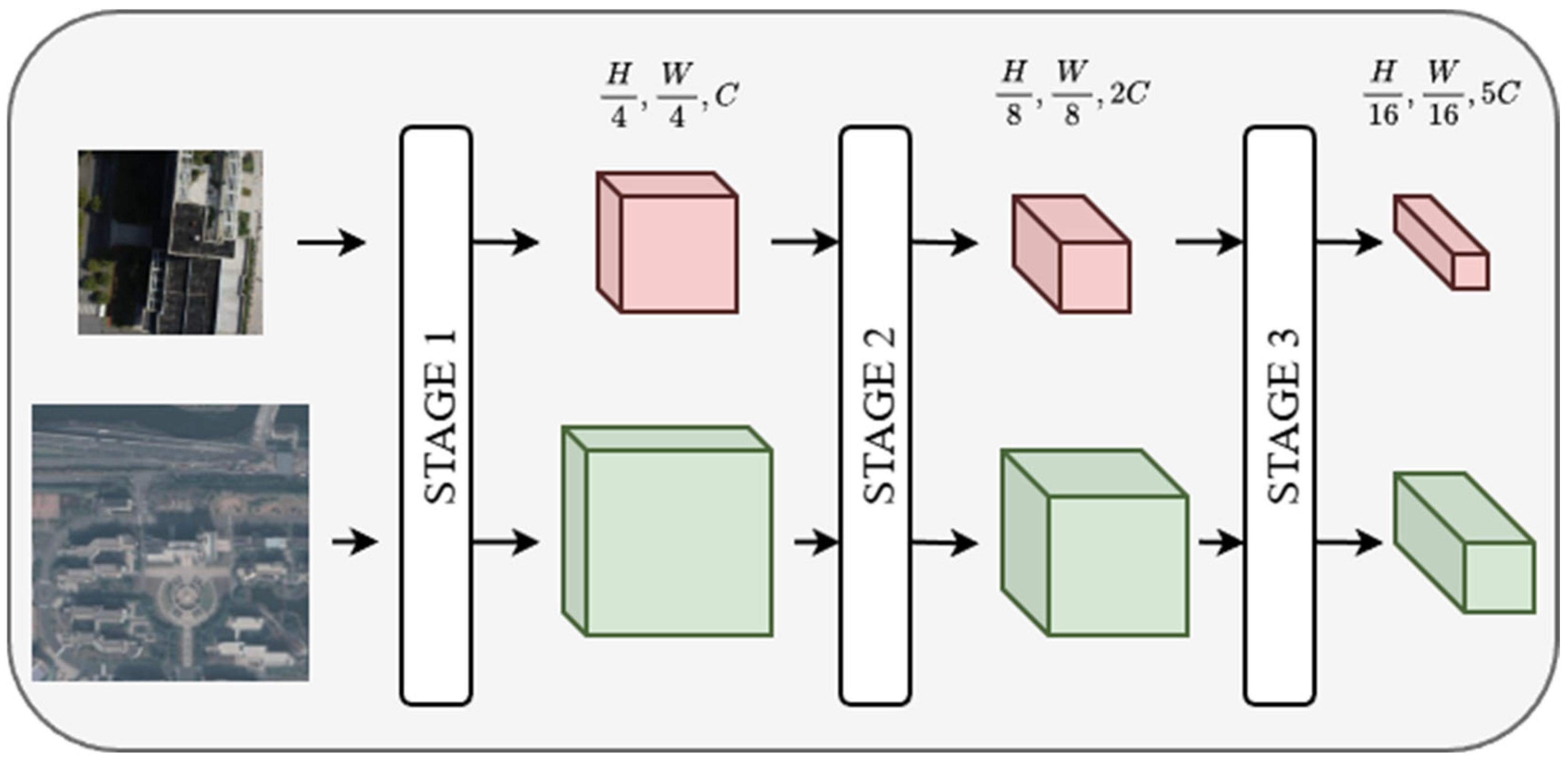
To conduct our experiments, we leveraged a pretrained OS-PCPVT [9] backbone as our feature extractor. OS-PCPVT is a transformer-based hierarchical network (outlined in Figure 3) that utilizes both self-attention and cross-attention to extract relevant features and their interactions early. Moreover, it is a dual-input network that processes both UAV and satellite images simultaneously.

Every stage of OS-PCPVT works as follows: Both inputs undergo a patch embedding operation, after which all tokens are concatenated and enter the transformer block. After the first transformer block, the positional encoding generation is performed and then the transformer block is applied N times. N values are 2, 4, and 6 for stages 1, 2, and 3 respectively. Just like PVT, OS-PCPVT has spatial reduction attention, which keeps the backbone light. In the transformer block, self-attention is performed for the UAV branch (keys, values and queries are sampled only from UAV input), and cross-attention is performed for the attention branch (keys and values are sampled from UAV and queries are sampled from satellite input). In such a way, the UAV branch exclusively models the UAV features, and the satellite branch models the interaction between the UAV and the satellite.

3.3. MuRDE-FPN

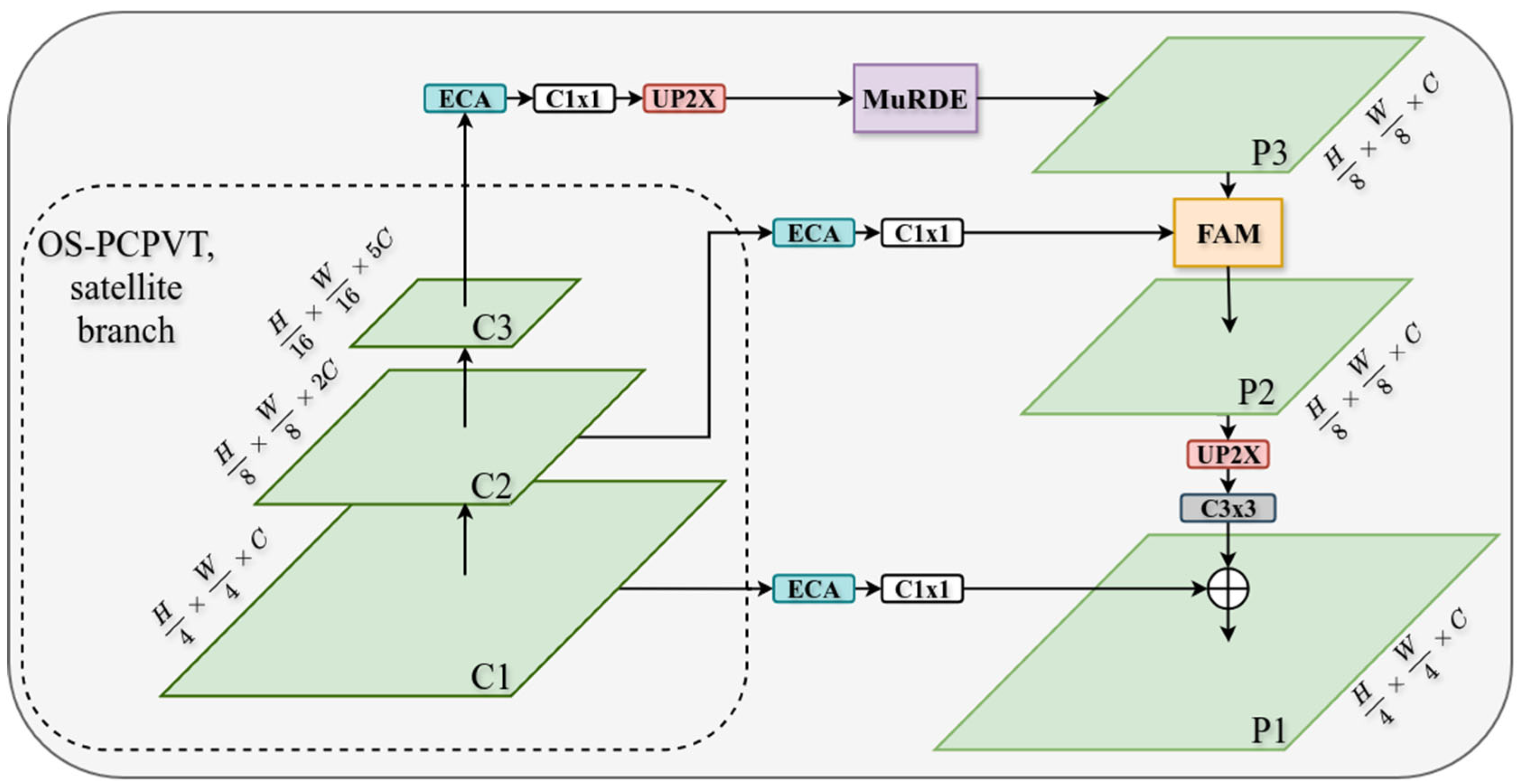
To keep our model lightweight, we limit ourselves to modeling only on the satellite branch from the OS-PCPVT backbone. We are able to do such modeling, given that the output from every stage in the satellite branch is constructed using cross-attention. In traditional FPN, the fusion of different scales is achieved as follows: each layer is unified with a convolutional layer with kernels of size 1, and the current and smaller (in terms of spatial dimensions) feature maps are upsampled and then added (or concatenated) with the previous layer. We aimed to enhance the classical FPN structure so it would better serve the FPI task. The central design principle of MuRDE-FPN is the selective refinement of the most semantically rich but spatially degraded feature level, rather than uniform enhancement across all pyramid levels. Additionally, traditional fusion methods (addition, concatenation, weighted fusion) are insufficient to model cross-scale interactions, and for this reason MuRDE-FPN also includes a spatial alignment module. The general outline of our architecture is visualized in Figure 4.

First, before lateral channel unification, we included an efficient channel attention (ECA) [41] operation for every feature map. ECA is a lightweight channel reweighting technique that adaptively suppresses or emphasizes channels without dimensionality reduction. In practice, ECA performs average pooling to extract channel-wise spatial descriptors, which then undergo one-dimensional convolution to capture local cross-channel interactions. We used channel-adaptive kernel selection, as proposed in the original implementation. Final channel-attention weights are normalized using the sigmoid function. Including ECA before channel unification allows for a more effective channel recalibration. We specifically chose this channel reweighting method in order to keep our final computational complexity almost intact, as ECA is very lightweight. After ECA, feature maps were unified to the same channel dimensionality (64 channels) using convolution with kernel size one.

Then, in our design, we included two key blocks: multi-receptive deformable enhancement (MuRDE) and feature alignment module (FAM). In both modules, deformable convolution (DCNv1) [42] is a key operator to achieve our goals. This type of convolution is an extension of the standard convolution with the inclusion of learnable spatial offsets. Output of such a convolution $y$ at a location $p$ is calculated:

$$y\left(p\right) = \sum _{k = 1}^{K}w\left(p_k\right)\cdot x\left(p+p_k+∆p\right)$$

(1)

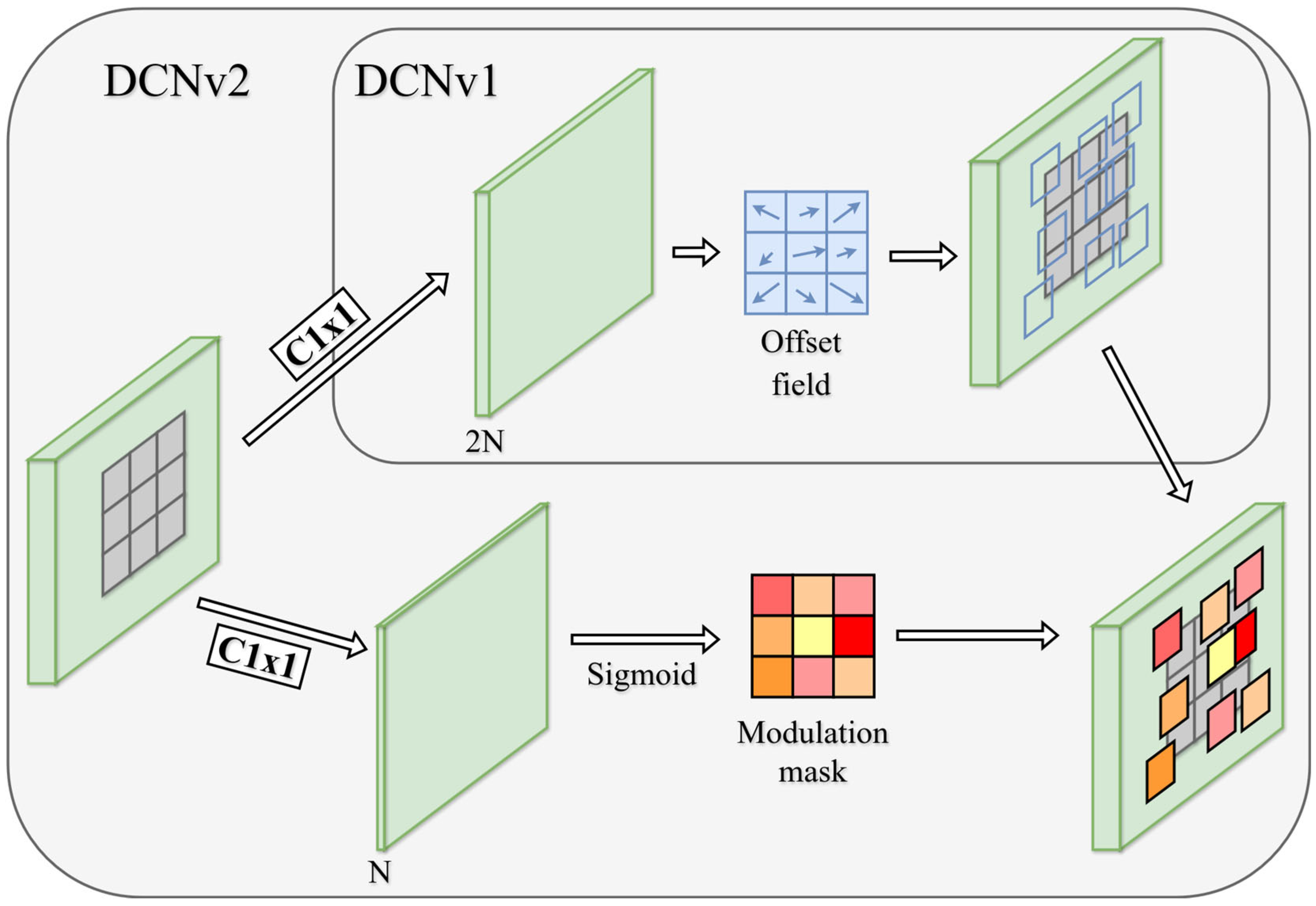
where $p_k$ is sampled from a regular convolution sampling grid at a location $k$, and $∆p_k$ denotes the learned offset for the same sampling point $k$. Then, $w\left(p_k\right)$ denotes learnable convolution weights at point $p_k$. In other words, this type of convolution is capable of adapting to input and capturing irregular patterns. In its second variant, DCNv2 [43], $∆m_k$ a modulating mask is introduced:

$$y\left(p\right) = \sum _{k = 1}^{K}w\left(p_k\right)\cdot x\left(p+p_k+∆p\right)\cdot △m_k$$

(2)

Modulation masks are also learnable, which means that DCNv2 is additionally capable of controlling the contribution of each sampling location. We outline the comparison between the computation of DCNv1 and DCNv2 in Figure 5. In our implementation, two lightweight convolution layers, both initialized with zero weights and bias, were used to generate offsets and a modulation mask. The deformable convolution samples feature at fractional locations using bilinear interpolation.

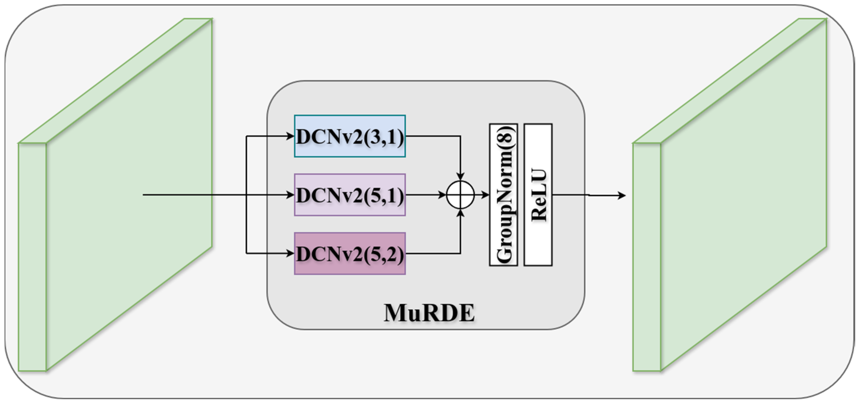
To enhance and refine the last layer of the backbone, we specifically designed the MuRDE block. While the last layer from the satellite branch in OS-PCPVT is most semantically rich, it suffers from spatial loss, since the original satellite input is downsampled 16 times. Because of this, we believe that the additional refinement and enhancement of such a feature map is beneficial. To achieve this, the MuRDE block uses DCNv2 as follows: Given an input feature map, different configurations of DCNv2 were computed. Configurations differ in kernel size and dilation, or, in other words, the MuRDE block is able to capture multiple resolutions. Outputs from every DCNv2 convolution were then fused by simple addition, followed by group normalization and the ReLU activation function (shown in Figure 6). The final configuration of the parameters in the MurDE block can be seen in Figure 6, and our final configuration of the MuRDE module includes convolutions that have receptive fields of 3 × 3, 5 × 5, and 9 × 9. In our implementation, DCNv2 groups were set to 1.

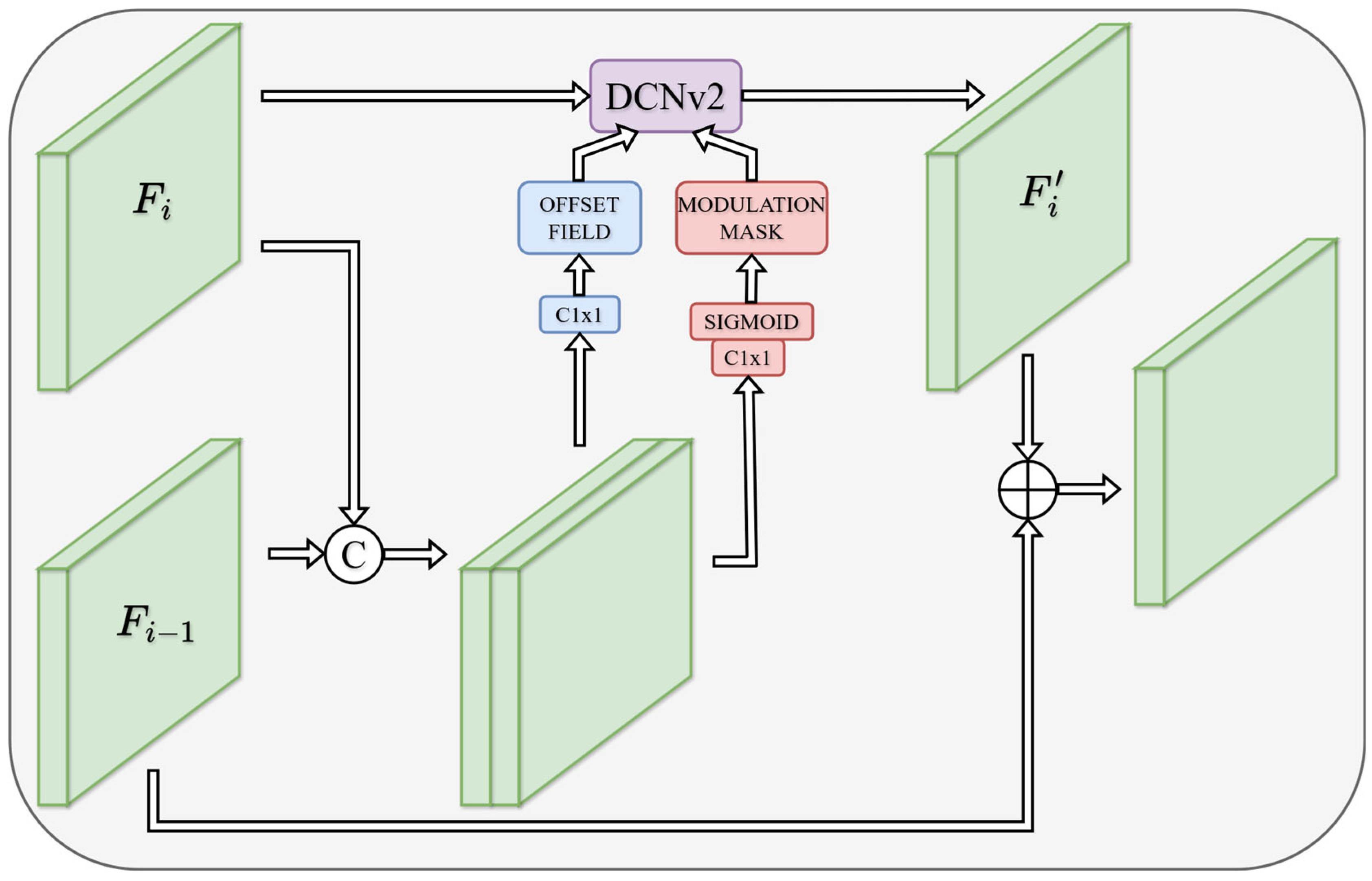
Inspired by [44,45,46,47], our final model also has a FAM block (Figure 7). We include FAM only to reduce the misalignment of the last two feature layers (or specifically, C2 output from OS-PCPVT and output from the MuRDE module), as in our case, including this module between the first two (C1 and C2) levels actually degraded the performance. In our implementation of FAM, we used DCNv2 with kernel of size 3, dilation and groups were set to 1.

FAM works as follows: Given two feature maps, those coming from deeper in the backbone are prone to more misalignment. To address this, the two feature maps are concatenated, and offsets and modulation masks are computed for the deformable convolution. Then, the map that suffers from more misalignment (in our case, output from the MuRDE block, as it was derived from a more downsampled feature layer) is refined withDCNv2, such that the now aligned map is fused with another map; in our case, simple addition was used.

3.4. Experimental Setup and Evaluation

Our experiments were conducted on an NVIDIA GeForce RTX 4090 GPU (manufactured by MSI, sourced in Vilnius, Lithuania). The experiments were implemented in Python 3.12.3 and PyTorch 2.5.0 with CUDA 12.4. To ensure a consistent training environment, we used a single seed (set to 42). Since a pretrained OS-PCPVT backbone was used throughout all of our experiments, we set discriminative learning rates: 5 × 10⁻⁵ for the backbone and 1 × 10⁻⁴ for the head and neck with the AdamW optimizer, with its parameters set to default values. To achieve optimal learning rate scheduling, our method uses MultiStepLRScheduler with milestones set to 10, 14, and 16 and the gamma parameter set to 0.2. We trained our model for 30 epochs, with a batch size of 8, using a Hanning window loss [39], with window size set to 33.

To evaluate other FPI methods on the UAV-Sat dataset, we opted not to use the same training hyperparameters as for our model but instead we followed procedures that these models use in their own setting as closely as possible. In other words, we kept the original network architectures, number of epochs, batch sizes, loss functions and their parameters, optimizers, schedulers and their respective parameters, learning rates, data normalization procedures, and input sizes. This was done in order to give each method the best shot possible, as, in training DL algorithms, the choice of various hyperparameters matters a lot, and we believe that each model was optimized best by their authors.

In line with the current FPI research, we evaluated our and other methods using RDS and meter-level accuracy (MA@K) metrics. RDS can be defined as:

$$RDS = e^{-k\times RD}$$

(3)

where k is a scaling factor (set to 10), and $RD$ is the relative distance between the predicted image location $\left(X_p, Y_p\right)$ and ground truth image coordinates $\left(X_g, Y_g\right)$:

$$RD = \sqrt{{\displaystyle \frac{{\left(\frac{dx}{w}\right)}^2+{\left(\frac{dy}{h}\right)}^2}{2}}}$$

(4)

where $dx = \left|X_p-X_g\right|$, $dy = \left|Y_p-Y_g\right|$, and $w$ and $h$ are the width and height of the image. In this way, RDS is a crucial metric for evaluating models’ performance at the pixel level and is resistant to image scale transformation. Note that higher values of RDS are better, and the score is distributed between 0 and 1. This is the main model optimization metric as well. However, RDS is not very helpful when evaluating real-life distance performance. For this reason, an additional metric, MA@K is defined as:

$$MA@K = {\displaystyle \frac{ {\sum }_{i = 1}^N{1}_{SD<Km}}{N}}$$

(5)

Here $1_{SD<Km}$ is a condition defined as:

$$1_{SD<Km}=\left\{\begin{array}{c}1, if SD<Km \\ 0, if SD\ge Km\end{array}\right.$$

(6)

where $SD$ denotes the distance in meters and $Km$ marks the chosen meter threshold. Note that $MA@k$ is sensitive to scale. For larger images, the resizing operation gives way to larger unit pixel values in meters. This in turn means that small distances between predicted and true pixel locations might be small, but meter distances are larger compared with smaller images.

We also introduce mean spatial distance (MSD), which is a derivative of SD. For the whole dataset, we define $MSD$ as:

$$MSD={\displaystyle \frac{1}{N}}\sum _{i = 1}^{N}S{D}_i = {\displaystyle \frac{1}{N}}\sum _{i = 1}^N\sqrt{\left(∆x_i^2+∆y_i^2\right)}$$

(7)

where $∆x_i$ and $∆y_i$ denote the distance between the ground truth and predicted points in horizontal and vertical directions expressed in meters for one sample. Just like $MA@k$, this metric is sensitive to the scale of the image and should not be used as a primary evaluation metric.

4. Experimental Results

In this section, we present our findings when comparing our approach with four other FPI methods—FPI, WAMF-FPI, OS-FPI and DCD-FPI. Two of these (FPI and WAMF-FPI) have an unshared backbone, where feature extraction is done independently and feature interaction modeling comes after. Others (OS-FPI, DCD-FPI, and MuRDE) have a shared backbone. Furthermore, OS-FPI and DCD-FPI have the same backbone as ours (OS-PCPVT), which makes such evaluation valuable in enabling the comparison of non-generic FPN-based methods. All methods are first compared on the UL14 dataset to ensure comparability with prior work and subsequently trained and tested on the UAV-Sat to assess robustness beyond the standard setting.

4.1. Evaluation of UL14 Dataset

Table 2. Comparison of different FPI methods, evaluated on the UL14 dataset. We report MA@k as a percentage. Bold indicates the best and underline indicates the second best performance.

Method	RDS	MA@3	MA@5	MA@20	Params (M)	GMACs
FPI [12]	57.22	-	18.63	57.67	43.33	14.58
WAMF-FPI [39]	65.33	12.49	26.99	69.73	47.47	13.36
OS-FPI [13]	76.25	22.81	44.31	82.52	14.25	14.31
DCD-FPI [17]	77.15	25.09	47.03	83.39	13.87	10.69
MuRDE-FPN	84.26	30.93	55.42	93.06	14.15	11.81

outlines the comparative performance on the UL14 dataset, and it is seen that our method, MuRDE, outperforms them all. Specifically, we outperform comparative models (OS-FPI and DCD-FPI) by 8.01 and 7.11 in RDS metric. Looking at the aggregated metrics, our method is also superior to DCD-FPI in meter accuracy at 3, 5, and 20 m by 5.84, 8.39 and 9.57 points respectively. While our method outperforms both of the two-stream methods and OS-FPI in terms of parameter count and giga multiply-accumulate operations (GMACs), DCD-FPI is still comparatively lighter. Specifically, our method is heavier by 0.28 M parameters and has 1.12 more GMACs than DCD-FPI. Nonetheless, we believe that such an increase in computational complexity is tolerable given the overall performance of MuRDE-FPN on the UL14 dataset.

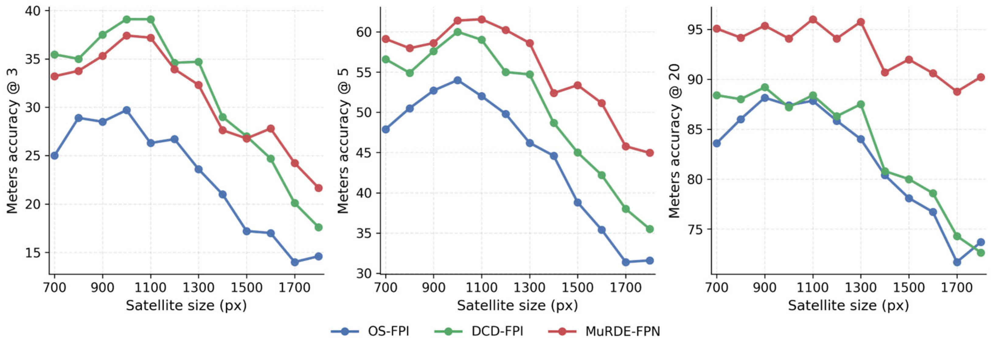
To provide a more extensive evaluation of UL14 and the impact of satellite size towards the precision metrics, Figure 8 illustrates the MA@k dependence on satellite image size to the performance of those methods that utilize the OS-PCPVT backbone. Interestingly, our model shows superior performance than DCD-FPI for the MA@3 metric for satellite maps that are smaller than a 1500 × 1500 resolution. However, MuRDE-FPN outperforms both OS-FPI and DCD-FPI in all other cases and in all other metrics.

4.2. Evaluation of UAV-Sat Dataset

To evaluate the performance of our method in a more general setting environment, we also provide a comparison of the UAV-Sat dataset (

Table 3. Comparison of different FPI methods, evaluated on the UAV-Sat dataset. We report MA@k as a percentage. Bold indicates the best, and underline indicates the second best performance.

Method	RDS	MSD	MA@100	MA@150	MA@200	MA@300
FPI [8]	37.61	217.21	15.98	29.06	41.74	77.54
WAMF-FPI [39]	43.95	199.14	20.92	36.64	50.56	81.41
OS-FPI [13]	59.03	185.16	25.03	42.28	57.57	84.98
DCD-FPI [17]	56.44	188.95	24.98	40.34	55.59	83.38
MuRDE-FPN	63.74	172.06	28.91	46.12	60.62	88.43

). Given the fact that the UAV-Sat dataset consists of high-altitude coverage and bigger map sizes, we report RDS as the main metric, but also additionally provide the MA@k metric for higher ranges than for the UL14 dataset. Given that the evaluated heatmaps in UAV-Sat cover a bigger area than those in UL14, we report MA@k starting at 100 m rather than 3 m. Such k ranges are also reported due to the fact that MSD varies from 172.06 to 217.21 for the compared methods. Table 3 showcases how all methods suffered a substantial decrease in performance when comparing RDS scores with those of the UL14 dataset: −19.61 for FPI, −21.38 for WAMF-FPI, −17.22 for OS-FPI, −20.71 for DCD-FPI, and −20.52 for MuRDE-FPN. The average decrease in performance is 19.89 RDS points, which attests to UAV-Sat difficulty. Even when evaluating different methods on such a dataset, our method outperforms comparative methods in the RDS metric: we see a 4.71 point increase when compared with OS-FPI and a 7.3 point increase when compared with DCD-FPI. Interestingly, the performance gap between OS-FPI and MuRDE is significantly lower when evaluated on the UAV-Sat dataset than on the UL14 dataset. Our method is also superior in MSD and MA@k metrics.

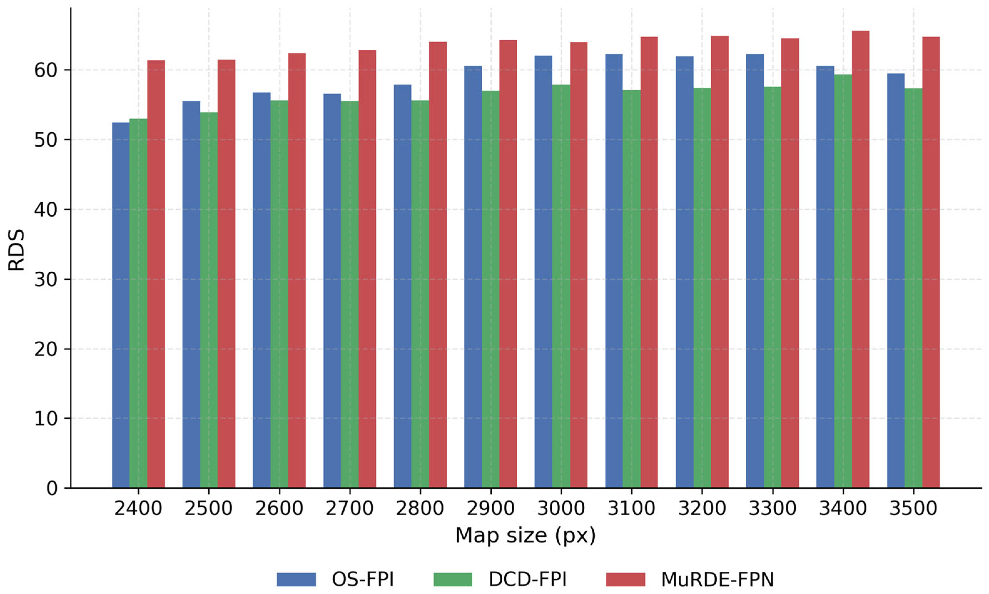
In Figure 9, the impact on RDS depending on satellite image size can be seen. In this regard, our method is also superior to the comparative methods (OS-FPI and DCD-FPI). It can be seen that the RDS performance on the UAV-Sat dataset remains more stable compared with other methods. For samples of different map sizes, we observe standard deviations of 1.4, 1.7, and 3.18 for our model, DCD-FPI and OS-FPI respectively. This is indicative of our model (and also DCD-FPI) being slightly more stable than OS-FPI under different satellite map size conditions.

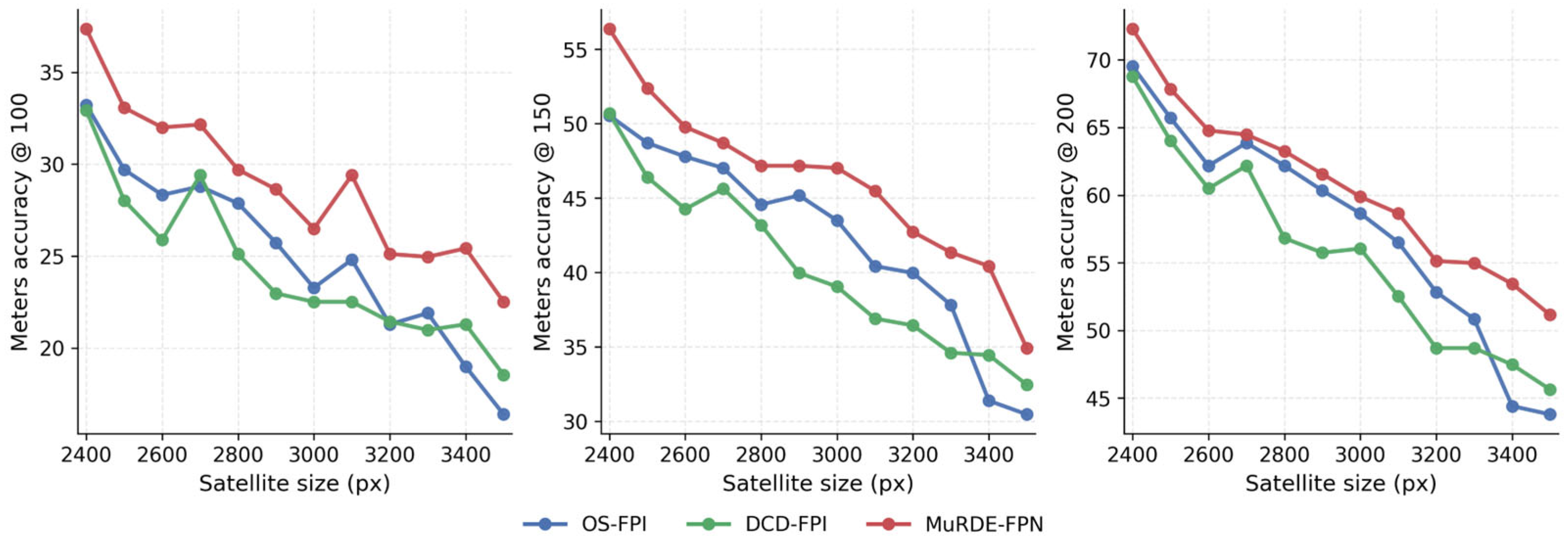
In Figure 10, the performance in precision metrics depending on satellite map size can be seen. When the performance is compared with the previously used UL14 dataset, we can see that the UAV-Sat dataset is far more challenging in terms of non-relative metrics. All compared models suffer from a sharp decline in MA@k as the map size increases, which is to be expected, as these metrics do not correct for the decreased resolution of bigger maps. Our proposed method performs better than OS-FPI and DCD-FPI in all cases, even MA@100 (which is similar to MA@3 in UL14 in terms of bin distribution). Additionally, differing from the results from the UL14 dataset, our method, while still better, is similar in its performance at MA@200 to OS-FPI and DCD-FPI.

Table 4. Comparison of different FPI methods, RDS performance, depending on altitude category. Bold indicates the best, and underline indicates the second best performance in the altitude group.

Method	RDS
	<500 m	>500 m
FPI [8]	40.42	34.78
WAMF-FPI [39]	48.22	39.64
OS-FPI [13]	62.87	55.16
DCD-FPI [17]	61.93	50.9
MuRDE-FPN	66.79	60.66

additionally provides insight into the performance when comparing high and very high altitude data. High altitude is defined when altitude ranges from 400 to 500 m, and very high, above 500 m. On average, we see a performance decrease with altitude when comparing models with the same backbone (OS-PCPVT): −6.14, −7.71, −11.3, −8.58, and −5.64 for MuRDE-FPN, OS-FPI, DCD-FPI, WAMF-FPI, and FPI respectively. This is not surprising, as data from higher altitudes contain more features inherently and are thus more difficult for all end-to-end methods.

5. Ablation Study

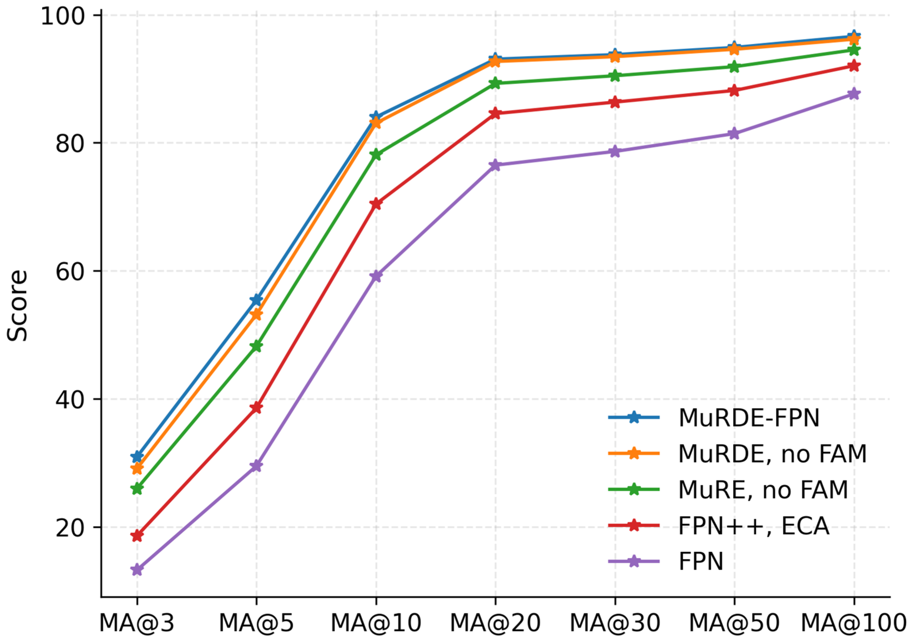
To further investigate the impact of different fusion, refinement, and enhancement strategies on the performance, we conducted an ablation analysis on the UL14 dataset. In the first analysis, we compare our strategies in an additive manner. We selected our baseline to be a simple FPN, as described in [29], and with FPN++ we denote a variant of traditional FPN, where an additional refinement convolution of kernel size 3 is added after upsampling. Next, we additively introduce our proposed steps: ECA, multi-receptive enhancement (MuRE), MuRDE, and the addition of FAM, but only to fuse the output of MuRE/MuRDE and C2. In MuRE, the enhancing logic is the same as our method, except we use classic convolutions here. General results of UL14 are shown in

Table 5. Comparison of methods evaluated on the UL14 dataset. The inclusion of a specific module is indicated by a + sign.

Method						RDS	MSD	GMACs	Params (M)
FPN	FPN++	ECA	MuRE	MuRDE	FAM
+						68.94	32.1	10.4	13.51
	+					76.12	21.88	11.24	13.62
	+	+				76.01	22.17	11.24	13.62
	+	+	+			80.64	16.81	11.71	13.82
	+	+		+		83.67	13.17	11.74	14.08
	+	+		+	+	84.26	12.21	11.81	14.15

.

It can be seen that almost every strategy improved performance. Most notably, the biggest increase in performance can be seen between FPN and FPN++ (+7.18) and an accumulative increase of +8.14 when comparing our final method with FPN++. Comparing FPN++ and FPN++ with ECA, we chose to include ECA in our final model because of slightly better performance in the 3 and 5 m range. MA@3 was observed at 18.6 and 18.37, and MA@5 was seen to be at 38.58 and 38.44 for FPN++ with ECA and FPN++ without ECA, respectively. The benefit of the MuRDE block is seen, as it gives an increase in performance by 7.57 when comparing it with FPN++ and ECA configurations. Finally, the choice of using DCNv2 compared with standard convolution is apparent, as MuRDE outperforms MuRE by 3.03 RDS points. Meter accuracies can be seen in Figure 11, and the same tendencies can be seen there as well. Regarding FAM feature fusion strategy, while the RDS increased by only 0.59 points, improvements can be specifically seen in the precision range (3–10 m).

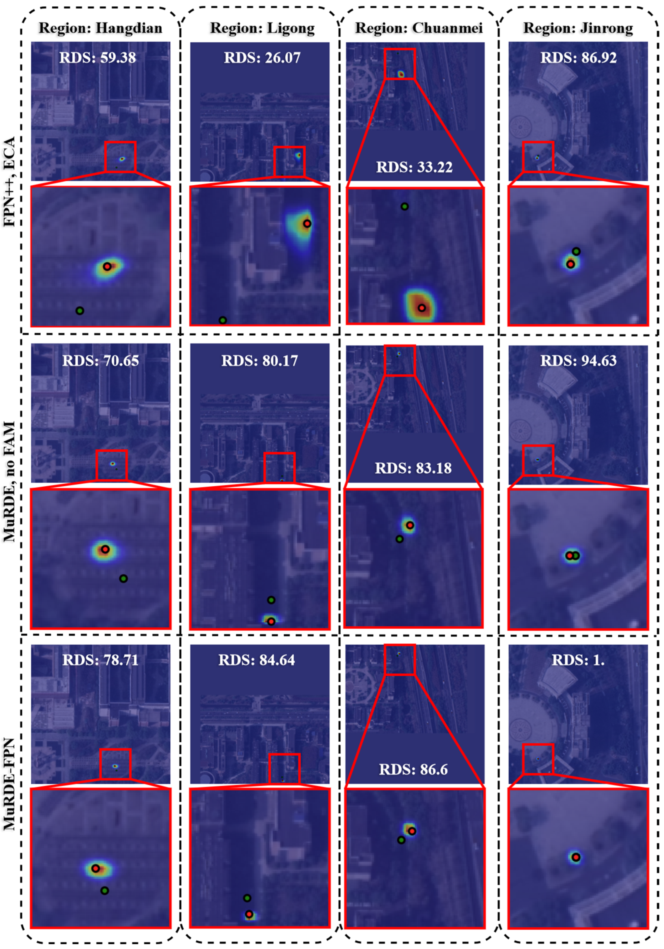
Additionally, we visualize the impact of different methods on the UL14 dataset in Figure 12. In the figure, the first line showcases the heatmap on the whole satellite image, and the second line showcases a zoomed-in view. We specifically visualize those cases where RDS improvements were observed (compared with FPN++, ECA configuration). In those cases, MuRDE and FAM blocks can be seen to be beneficial not only in reducing overall distance between predicted and ground truth locations but also in concentrating the predicted area.

To investigate how kernels of different sizes and dilations (and therefore kernels of different receptive fields) affect the performance, we also conducted additional analysis. In this ablation experiment, we limited ourselves to kernels of sizes 3 and 5, given that the final model should be as light as possible, and kernels of smaller sizes are computationally cheaper.

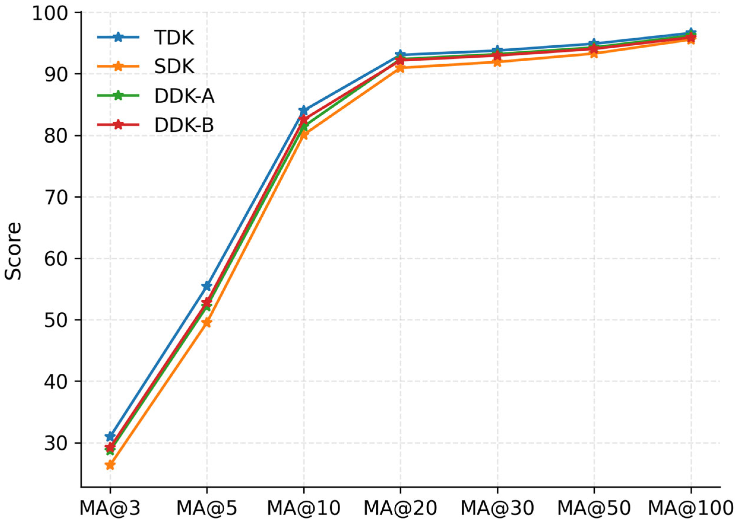
The results are shown in

Table 6. Comparison of MuRDE module configuration impact. The inclusion of a specific module is indicated by a + sign.

Method				RDS	MSD	GMACs	Params (M)
SDK	DDK-A	DDK-B	TDK
+				81.96	14.69	11.26	13.70
	+			83.30	13.23	11.54	13.92
		+		83.27	13.60	11.54	13.92
			+	84.26	12.21	11.81	14.15

, and we compare experiments with the following kernel configurations: single deformable kernel of size 3 and dilation 1 (SDK); double deformable kernel of sizes 3 and 5 and dilations 1 and 1 respectively (DDK-A); double deformable kernel of sizes 3 and 5 and dilations 1 and 2 (DDK-B); triple kernel consisting of size 3, 5, 5 convolutions and 1, 1, 2 dilations (TDK). In such a way we constructed four different receptive field MuRDE modules: size 3 receptive field (SDK), size 3 and 5 receptive fields (DDK-A), size 3 and 9 receptive fields (DDK-B) and size 3, 5, 9 receptive field modules (TDK, our final model configuration).

Figure 13 visualizes the meter metrics for the MuRDE configuration, and it can be seen that, just like the increase in RDS, these metrics increased as well when comparing single, double, and triple kernel configurations.

6. Conclusions

This work presents MuRDE-FPN, a decoder-centered UAV localization strategy for the FPI task. On the standard UL14 benchmark, MuRDE-FPN achieved an RDS of 84.26 and improved same-backbone baselines (OS-FPI and DCD-FPI) by +8.01 and +7.11 RDS, respectively, while also increasing meter-level accuracies. We additionally introduce a UAV-Sat dataset that is intended to extend the findings to higher altitudes and bigger search area scenarios. On this dataset, MuRDE-FPN attained RDS 63.74 and outperformed OS-FPI and DCD-FPI by +4.71 and +7.30 RDS, respectively, indicating generalization beyond the UL14 setting. Additionally, our model achieved 60.66 RDS in very high-altitude conditions, which was +5.5 increase in RDS compared with the second best, OS-FPI, method. The proposed improvements come with a moderate increase in complexity relative to DCD-FPI (+0.28 M parameters and +1.12 GMACs), while remaining substantially lighter than two-branch alternatives.

Nonetheless, the present study has some important limitations. We did not evaluate our or other methods in difficult conditions, such as UAV image conclusions or extremely difficult scenarios (rainy, foggy or snowy weather). Moreover, we did not quantify robustness to real flight degradations. Future work will therefore focus on extensive evaluation under such conditions and on integration of the proposed vision-based localization output as an aiding signal for navigation pipelines in GNSS-challenged scenarios.

7. Discussion

In our work, we treated the FPI task as a mixture of target tracking and segmentation, as, on the one hand, finding point in an image is targeting but, on the other hand, precision positioning should restore the final map as a dense heatmap. To enrich the precise UAV positioning literature, we propose our MuRDE-FPN model, which utilizes a one-stream backbone with a custom-designed FPN decoder. Our model architecture, MuRDE-FPN, addresses key challenges of multi-scale feature enrichment and spatial misalignment. By introducing the MuRDE module at the deepest stage of the feature pyramid, we enhance high-level semantic representations, and FAM enables the adaptive merging of the enriched features while preserving spatial consistency. We believe that our findings indicate the potential of custom FPN refining methods in the FPI task, with a special focus on specific scales, as with our method we observed the improved performance of UAV localization in two datasets: UL14 and UAV-Sat. The improvements were seen in both relative (RDS) and absolute (MSD, MA@k) metrics. We also found that our method improves localization with bigger satellite search maps and high altitudes compared with other methods.

We are, however, limited by our backbone design, and for this reason, our implications can be extended only to a specific setting: one-stream hierarchical backbone designs, in which cross-modal modeling is done at every stage. Even then, given the improvements in performance, some of our design choices can be integrated into different backbones. For instance, Chen et al. [14] noticed that effective usage of last feature significantly enhanced performance compared with other methods. Our findings are very similar, as we note an increase in performance when enhancing the most semantically rich layer as well. We adopt a multi-receptive approach and observe a performance increase when using non-deformable convolution as well. However, it is still unclear what could be the magnitude of improvement if such an approach would be integrated into other backbones, as other FPI works [14,15,16] note that the backbone design by itself impacts the performance as well.

Model size and memory requirements matter a lot in UAV applications since onboard deployment dictates a scarcity of resources. While our method is much lighter in terms of model size than the compared two-branch methods, some achieved similar results on the UL14 with lower computational cost [14,15,16]. In the future, we will address this issue with the smallest decrease in performance possible. In addition to popular model design solutions (model pruning techniques) to reduce the computational overhead, we will also aim to investigate different training strategies (knowledge distillation, deep supervision, contrastive pretraining) for optimal performance.

We also propose a new dataset for proper evaluation of the FPI methods. While similar datasets (derived from UAV-VisLoc) were proposed before [14,16,18], our derivation is unique in that the validation set is similar in its difficulty compared with the UL14 dataset and enables evaluation on much bigger satellite images. Our dataset also contains high altitude UAV footage, which makes it inherently more diverse for practical UAV applications. There are, however, some gaps that this dataset is unable to address. It is not clear how the end-to-end methods perform overall under different quality data. In particular, a gap exists when evaluating images with visible/substantial change or occlusion, e.g., in areas that experience rapid urbanization, destruction, climate change, night-time footage, motion artefacts, or seasonal variation. In the future, we will aim to address this gap with additional synthetic expansion (e.g., using generative adversarial networks) of our dataset to include such difficult footage.

References

1. Manoj, H.M.; Shanthi, D.L.; Lakshmi, B.N.; Archana, K.J.; Venkata Naga Jyothi, E.; Archana, K. AI-Driven Drone Technology and Computer Vision for Early Detection of Crop Disease in Large Agricultural Areas. Sci. Rep. 2025, 16, 2479. [Google Scholar] [CrossRef] [PubMed]
2. Shakhatreh, H.; Sawalmeh, A.H.; Al-Fuqaha, A.; Dou, Z.; Almaita, E.; Khalil, I.; Othman, N.S.; Khreishah, A.; Guizani, M. Unmanned Aerial Vehicles (UAVs): A Survey on Civil Applications and Key Research Challenges. IEEE Access 2019, 7, 48572–48634. [Google Scholar] [CrossRef]
3. Shayea, I.; Dushi, P.; Banafaa, M.; Rashid, R.A.; Ali, S.; Sarijari, M.A.; Daradkeh, Y.I.; Mohamad, H. Handover Management for Drones in Future Mobile Networks—A Survey. Sensors 2022, 22, 6424. [Google Scholar] [CrossRef] [PubMed]
4. Zheng, T.; Xu, A.; Xu, X.; Liu, M. Modeling and Compensation of Inertial Sensor Errors in Measurement Systems. Electronics 2023, 12, 2458. [Google Scholar] [CrossRef]
5. Lowe, D. Object Recognition from Local Scale-Invariant Features. In Proceedings of the Seventh IEEE International Conference on Computer Vision, Kerkyra, Greece, 20–27 September 1999; pp. 1150–1157. [Google Scholar] [CrossRef]
6. Liu, Y.; Wang, Y.; Wang, D.; Wu, W.; Li, X.X.; Sun, W.; Ren, X.; Song, H. A Scalable Benchmark to Evaluate the Robustness of Image Stitching under Simulated Distortions. Sci. Rep. 2025, 15, 32816. [Google Scholar] [CrossRef]
7. Sarlin, P.-E.; DeTone, D.; Malisiewicz, T.; Rabinovich, A. SuperGlue: Learning Feature Matching with Graph Neural Networks. In Proceedings of the IEEE/CVF Conference on Computer Vision and Pattern Recognition, Seattle, WA, USA, 13–19 June 2020. [Google Scholar] [CrossRef]
8. Gong, F.; Hao, J.; Du, C.; Wang, H.; Zhao, Y.; Yu, Y.; Ji, X. FIM-JFF: Lightweight and Fine-Grained Visual UAV Localization Algorithms in Complex Urban Electromagnetic Environments. Information 2025, 16, 452. [Google Scholar] [CrossRef]
9. Ding, L.; Zhou, J.; Meng, L.; Long, Z. A Practical Cross-View Image Matching Method between UAV and Satellite for UAV-Based Geo-Localization. Remote Sens. 2021, 13, 47. [Google Scholar] [CrossRef]
10. Cui, Z.; Zhou, P.; Wang, X.; Zhang, Z.; Li, Y.; Li, H.; Zhang, Y. A Novel Geo-Localization Method for UAV and Satellite Images Using Cross-View Consistent Attention. Remote Sens. 2023, 15, 4667. [Google Scholar] [CrossRef]
11. Xu, Y.; Dai, M.; Cai, W.; Yang, W. Precise GPS-Denied UAV Self-Positioning via Context-Enhanced Cross-View Geo-Localization. arXiv 2025, arXiv:2502.11408. [Google Scholar] [CrossRef]
12. Dai, M.; Chen, J.; Lu, Y.; Hao, W.; Zheng, E. Finding Point with Image: An End-to-End Method for Vision-Based UAV Localization. arXiv 2022, arXiv:2208.06561. [Google Scholar] [CrossRef]
13. Chen, J.; Zheng, E.; Dai, M.; Chen, Y.; Lu, Y. OS-FPI: A Coarse-to-Fine One-Stream Network for UAV Geolocalization. IEEE J. Sel. Top. Appl. Earth Obs. Remote Sens. 2024, 17, 7852–7866. [Google Scholar] [CrossRef]
14. Chen, N.; Fan, J.; Yuan, J.; Zheng, E. OBTPN: A Vision-Based Network for UAV Geo-Localization in Multi-Altitude Environments. Drones 2025, 9, 33. [Google Scholar] [CrossRef]
15. Fan, J.; Zheng, E.; He, Y.; Yang, J. A Cross-View Geo-Localization Algorithm Using UAV Image and Satellite Image. Sensors 2024, 24, 3719. [Google Scholar] [CrossRef] [PubMed]
16. Ju, C.; Xu, W.; Chen, N.; Zheng, E. An Efficient Pyramid Transformer Network for Cross-View Geo-Localization in Complex Terrains. Drones 2025, 9, 379. [Google Scholar] [CrossRef]
17. He, Y.; Chen, F.; Chen, J.; Fan, J.; Zheng, E. DCD-FPI: A Deformable Convolution-Based Fusion Network for Unmanned Aerial Vehicle Localization. IEEE Access 2024, 12, 129308–129318. [Google Scholar] [CrossRef]
18. Tian, L.; Shen, Q.; Gao, Y.; Wang, S.; Liu, Y.; Deng, Z. A Cross-Mamba Interaction Network for UAV-to-Satellite Geolocalization. Drones 2025, 9, 427. [Google Scholar] [CrossRef]
19. Yao, Y.; Sun, C.; Wang, T.; Yang, J.; Zheng, E. UAV Geo-Localization Dataset and Method Based on Cross-View Matching. Sensors 2024, 24, 6905. [Google Scholar] [CrossRef]
20. Vaswani, A.; Shazeer, N.; Parmar, N.; Uszkoreit, J.; Jones, L.; Gomez, A.N.; Kaiser, Ł.; Polosukhin, I. Attention Is All You Need. arXiv 2017, arXiv:1706.03762. [Google Scholar] [CrossRef]
21. Dosovitskiy, A.; Beyer, L.; Kolesnikov, A.; Weissenborn, D.; Zhai, X.; Unterthiner, T.; Dehghani, M.; Minderer, M.; Heigold, G.; Gelly, S.; et al. An Image Is Worth 16 × 16 Words: Transformers for Image Recognition at Scale. arXiv 2021, arXiv:2010.11929. [Google Scholar] [CrossRef]
22. Wang, W.; Xie, E.; Li, X.; Fan, D.-P.; Song, K.; Liang, D.; Lu, T.; Luo, P.; Shao, L. Pyramid Vision Transformer: A Versatile Backbone for Dense Prediction without Convolutions. arXiv 2021, arXiv:2102.12122. [Google Scholar] [CrossRef]
23. Liu, Z.; Lin, Y.; Cao, Y.; Hu, H.; Wei, Y.; Zhang, Z.; Lin, S.; Guo, B. Swin Transformer: Hierarchical Vision Transformer Using Shifted Windows. arXiv 2021, arXiv:2103.14030. [Google Scholar] [CrossRef]
24. Chu, X.; Tian, Z.; Wang, Y.; Zhang, B.; Ren, H.; Wei, X.; Xia, H.; Shen, C. Twins: Revisiting the Design of Spatial Attention in Vision Transformers. arXiv 2021, arXiv:2104.13840. [Google Scholar] [CrossRef]
25. Wang, W.; Xie, E.; Li, X.; Fan, D.-P.; Song, K.; Liang, D.; Lu, T.; Luo, P.; Shao, L. PVT v2: Improved Baselines with Pyramid Vision Transformer. Comput. Vis. Media 2022, 8, 415–424. [Google Scholar] [CrossRef]
26. Wang, Q.; Zhang, J.; Yang, K.; Peng, K.; Stiefelhagen, R. MatchFormer: Interleaving Attention in Transformers for Feature Matching. arXiv 2022, arXiv:2203.09645. [Google Scholar] [CrossRef]
27. Sun, J.; Shen, Z.; Wang, Y.; Bao, H.; Zhou, X. LoFTR: Detector-Free Local Feature Matching with Transformers. In Proceedings of the IEEE/CVF Conference on Computer Vision and Pattern Recognition, Nashville, TN, USA, 20–25 June 2021; pp. 8918–8927. [Google Scholar] [CrossRef]
28. Ye, B.; Chang, H.; Ma, B.; Shan, S.; Chen, X. Joint Feature Learning and Relation Modeling for Tracking: A One-Stream Framework. In Proceedings of the European Conference on Computer Vision, Tel Aviv, Israel, 23–27 October 2022; pp. 341–357. [Google Scholar] [CrossRef]
29. Lin, T.-Y.; Dollár, P.; Girshick, R.; He, K.; Hariharan, B.; Belongie, S. Feature Pyramid Networks for Object Detection. In Proceedings of the IEEE Conference on Computer Vision and Pattern Recognition, Honolulu, HI, USA, 21–26 July 2017; pp. 936–944. [Google Scholar] [CrossRef]
30. Liu, S.; Qi, L.; Qin, H.; Shi, J.; Jia, J. Path Aggregation Network for Instance Segmentation. arXiv 2018, arXiv:1803.01534. [Google Scholar] [CrossRef]
31. Ghiasi, G.; Lin, T.-Y.; Pang, R.; Le, Q.V. NAS-FPN: Learning Scalable Feature Pyramid Architecture for Object Detection. In Proceedings of the IEEE/CVF Conference on Computer Vision and Pattern Recognition, Long Beach, CA, USA, 15–20 June 2019; pp. 7029–7038. [Google Scholar] [CrossRef]
32. Tan, M.; Pang, R.; Le, Q.V. EfficientDet: Scalable and Efficient Object Detection. In Proceedings of the IEEE/CVF Conference on Computer Vision and Pattern Recognition, Seattle, WA, USA, 13–19 June 2020; pp. 10778–10787. [Google Scholar] [CrossRef]
33. Sun, G.; Jiang, X.; Lin, W. DBEENet: Dual-Branch Edge-Enhanced Network for Semantic Segmentation of USV Maritime Images. Ocean Eng. 2025, 341, 122731. [Google Scholar] [CrossRef]
34. Xie, C.; Li, M.; Zeng, H.; Luo, J.; Zhang, L. MaSS13K: A Matting-Level Semantic Segmentation Benchmark. arXiv 2025, arXiv:2503.18364. [Google Scholar] [CrossRef]
35. Thuan, N.H.; Oanh, N.T.; Thuy, N.T.; Perry, S.; Sang, D.V. RaBiT: An Efficient Transformer Using Bidirectional Feature Pyramid Network with Reverse Attention for Colon Polyp Segmentation. arXiv 2023, arXiv:2307.06420. [Google Scholar] [CrossRef]
36. Zhang, R.; Xie, M.; Liu, Q. CFRA-Net: Fusing Coarse-to-Fine Refinement and Reverse Attention for Lesion Segmentation in Medical Images. Biomed. Signal Process. Control 2025, 109, 107997. [Google Scholar] [CrossRef]
37. Zhou, G.; Xu, Q.; Liu, Y.; Liu, Q.; Ren, A.; Zhou, X.; Li, H.; Shen, J. Lightweight Multiscale Feature Fusion and Multireceptive Field Feature Enhancement for Small Object Detection in Aerial Images. IEEE Trans. Geosci. Remote Sens. 2025, 63, 5640213. [Google Scholar] [CrossRef]
38. Touvron, H.; Cord, M.; Douze, M.; Massa, F.; Sablayrolles, A.; Jégou, H. Training Data-Efficient Image Transformers and Distillation through Attention. arXiv 2020, arXiv:2012.12877. [Google Scholar] [CrossRef]
39. Wang, G.; Chen, J.; Dai, M.; Zheng, E. WAMF-FPI: A Weight-Adaptive Multi-Feature Fusion Network for UAV Localization. Remote Sens. 2023, 15, 910. [Google Scholar] [CrossRef]
40. Xu, W.; Yao, Y.; Cao, J.; Wei, Z.; Liu, C.; Wang, J.; Peng, M. UAV-VisLoc: A Large-Scale Dataset for UAV Visual Localization. arXiv 2024, arXiv:2405.11936. [Google Scholar] [CrossRef]
41. Wang, Q.; Wu, B.; Zhu, P.; Li, P.; Zuo, W.; Hu, Q. ECA-Net: Efficient Channel Attention for Deep Convolutional Neural Networks. In Proceedings of the IEEE/CVF Conference on Computer Vision and Pattern Recognition, Seattle, WA, USA, 13–19 June 2020; pp. 11531–11539. [Google Scholar] [CrossRef]
42. Dai, J.; Qi, H.; Xiong, Y.; Li, Y.; Zhang, G.; Hu, H.; Wei, Y. Deformable Convolutional Networks. In Proceedings of the IEEE International Conference on Computer Vision, Venice, Italy, 22–29 October 2017; pp. 764–773. [Google Scholar] [CrossRef]
43. Zhu, X.; Hu, H.; Lin, S.; Dai, J. Deformable ConvNets v2: More Deformable, Better Results. arXiv 2018, arXiv:1811.11168. [Google Scholar] [CrossRef]
44. Dong, X.; Qin, Y.; Fu, R.; Gao, Y.; Liu, S.; Ye, Y.; Li, B. Multiscale Deformable Attention and Multilevel Features Aggregation for Remote Sensing Object Detection. IEEE Geosci. Remote Sens. Lett. 2022, 19, 6510405. [Google Scholar] [CrossRef]
45. Fu, X.; Yuan, Z.; Yu, T.; Ge, Y. DA-FPN: Deformable Convolution and Feature Alignment for Object Detection. Electronics 2023, 12, 1354. [Google Scholar] [CrossRef]
46. Huang, S.; Lu, Z.; Cheng, R.; He, C. FaPN: Feature-Aligned Pyramid Network for Dense Image Prediction. In Proceedings of the IEEE/CVF International Conference on Computer Vision, Montreal, QC, Canada, 10–17 October 2021; pp. 844–853. [Google Scholar] [CrossRef]
47. Li, J.; Wang, Q.; Dong, H. BAFPN: Bidirectionally Aligning Features to Improve Object Localization Accuracy in Remote Sensing Images. Appl. Intell. 2025, 55, 1071. [Google Scholar] [CrossRef]
Figure 1. UAV and satellite views from the UL14 and UAV-Sat datasets. Purple outline indicates pair from UL14 dataset and blue indicates from UAV-Sat dataset.
Drones 10 00162 g001
Figure 2. RSC visualization. Red star denotes true location of UAV; green denotes center coordination of an augmented image.
Drones 10 00162 g002
Figure 3. General outline of the OS-PCPVT [13] backbone. Red layers indicate UAV branch; green ones indicate satellite branch.
Drones 10 00162 g003
Figure 4. Our method, MuRDE-FPN. C1×1 and C3×3 denote convolutional layers with kernel sizes 1 and 3, respectively; UP2X marks a feature upsampling operation using bilinear upsampling. ECA marks efficient channel attention. C equals 64 channels.
Drones 10 00162 g004
Figure 5. DCNv1 and DCNv2 comparison. N and 2N denote the number of channels, where N is kernel size squared.
Drones 10 00162 g005
Figure 6. MuRDE block. Numbers in the DCNv2 blocks denote the specific kernel size and dilation configurations. Number in GroupNorm block indicates the number of groups in group normalization layer.
Drones 10 00162 g006
Figure 7. FAM block.
Drones 10 00162 g007
Figure 8. Impact on performance depending on satellite template size, evaluated on the UL14 dataset. We compare methods with the same backbone (OS-PCPVT): OS-FPI [13], DCD-FPI [17], and ours, MuRDE-FPN.
Drones 10 00162 g008
Figure 9. Impact on performance depending on satellite template size; RDS evaluated on the UAV-Sat dataset. We compare methods with the same backbone (OS-PCPVT): OS-FPI [13], DCD-FPI [17], and ours, MuRDE-FPN.
Drones 10 00162 g009
Figure 10. Impact on MA@k performance depending on satellite template size; evaluated on UAV-Sat dataset. We compare methods with the same backbone (OS-PCPVT): OS-FPI [13], DCD-FPI [17], and ours, MuRDE-FPN.
Drones 10 00162 g010
Figure 11. MA@k metrics with different network configurations.
Drones 10 00162 g011
Figure 12. Heatmap visualization. Green dot denotes true location; red dot denotes predicted. RDS denotes RDS for the specific satellite map visualized.
Drones 10 00162 g012
Figure 13. MA@k metric using different MuRDE kernel configurations.
Drones 10 00162 g013