A Machine Learning Model Relating Xrain and Rain Gauge ^†

Abstract

In the last decade, rainfall radars have been deployed at volcanoes such as Mt. Merapi in Indonesia and can even cover a whole country such as in Japan, where the X-Rain (eXtended Radar Information network) product has been available for local research. However, the linkage between rain gauge data and spatial radar data (over a 250 m × 250 m grid) still presents discrepancies, and these challenges are particularly acute in regions of high local-topographic variations such as at Mount Unzen in Japan. As the volcano is located in the Shimabara peninsula, it is surrounded by the sea, with a topography locally rising to 1483 m. To improve the forecast and to better understand the triggering mechanisms of lahars (volcanic debris-flows) at Mount Unzen, quantifying the spatial distribution of rainfalls is essential, and first, it is important to understand how data taken locally by rain gages relate to spatial radar data. Because empirical models have not been able to show any clear correlation, the present contribution has been developing a neural network with two hidden layers that takes into account the rainfall per hour, the temperature and the wind speed and direction. The model takes a logistic activation function, and the loss function is optimized using the Mean Squared Errors and the Mean Absolute Error. The choice of the activation function and the optimizer is the result of running several combinations of optimization functions with different activation functions. Once the best fit was chosen, the sigmoid with a SGD (Stochastic Gradient Descent) optimizer was chosen, and when training the model for 120 cycles, Shimabara station and the Xrain data showed an error of <4 mm rainfall, while at the Unzen summit, even after 300 cycles, the validation error remained at 8 mm while the training loss was <4 mm. This shows that location specific functions might be necessary for each location, not only taking into account the weather data but also the local topographic variability and the topographic position on slopes.

1. Introduction

Stratovolcanoes’ eruptions create pyroclasts of sizes varying from ash to several meters clasts with events ranging from valley-size pyroclastic density currents and surges [1,2,3,4] to large explosions that can even trigger tsunamis (e.g., the prehistoric eruptions in Alaska [5]). These deposits are then remobilized over time—or instantly—by rainfall and transported further downstream, forming lahars [6,7], where mixtures of blocks and sediment and water flow in a “fluid manner” in and from valleys on volcanoes [8,9]. Lahars can be triggered by a variety of processes but are dominantly rainfall-triggered, a process well-studied in South America at Colima Volcano [10] at Popocatepetl [11], or at Cotopaxi Volcano [12], for instance. In East Asia, Indonesia, the Philippines and Japan have provided numerous case studies, e.g., Merapi Volcano in Indonesia [6,7,13], Semeru Volcano in Indonesia [14,15], etc.

One of the research gaps that remains, despite this large breadth of research, is the establishment of a predictive level of relations between rainfalls and lahars. This is essential for scientific and applied hazards and disaster risk purposes as well. Unfortunately, the rain gauges are never in the exact location where rainfall occurs, and the several-centimeter squares of the rain gauge are not representative of rainfalls that present high-spatial variability. To fill this gap, rainfall radar has been developed, notably by Japan, and applied to volcanoes such as Merapi Volcano [16]; however, the significance of the radar data in comparison with rain gauge data have not been assessed systematically as of yet, and the radar data have just been used to find thresholds of lahars [17] and only calibrated using mathematical models. Unfortunately, these relations do not address the problems of each site-location variability due to topographic and meso-scale level atmospheric conditions that are site-specific as well.

Consequently, the present contribution, therefore, aims to simulate the relation between rain gauge data and Xrain radar data so that periods, when no radar data existed, could be simulated back and then used to improve the simulation of rainfall-lahars’ triggering processes.

2. Research Location, Data and Methods

2.1. Research Location

The present research occurred at Shimabara peninsula in South Japan (Figure 1). Shimabara peninsula is dominated by Unzen Volcano, which last erupted in 1991–1995 following a long slumber. This eruption occurred at the Fugen-Dake, and a hundred years ago, a major flank collapse at Mt. Mayuyama (Figure 1) had then triggered a tsunami that took the lives of 15,000.

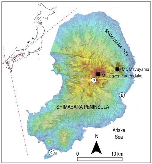
Figure 1. The location of the study area and the location of the three rain gauges: (a) Unzen, (b) Kuchinozu and (c) Shimabara.

2.2. Data and Method

To reach this goal, a neural network model was programmed in Python programming environment, starting from a set of data collected at Unzen Volcano, starting from rain gauge and rainfall radar data (Figure 1). ANN (Artificial Neural Network) is a popular method used to predict rainfall from rain gauges [18]. Therefore, a similar type of model was chosen to link the spatial distribution of the representation of the rainfall (Xrain radar data) to the rain gauge data.

Moreover, because the local terrain and other geographic factors influence the rainfall beyond what the rain gauge data can record, we posited that a BPNN (Backward Propagation Neural Nework) model was appropriate to integrate these different factors.

The model uses meteorological data from the Japan Meteorological Agency and rainfall data from the Xrain radar from 2018 to 2021. We built the model using the keras library in python, tuning the parameters until the result was good enough.

2.3. Data Preparation

The meteorological data was downloaded from the Japan Meteorological Agency website, and included hourly rainfall, wind speed, direction and temperature from 2018 to 2021 at three observation stations named Unzen, Kuchimozu and Shimabara, around the target sites. The Xrain data (the Japanese rainfall radar) were obtained from the Ministry of Land Infrastructure Transport and Tourism of Japan. The data was integrated over a regular time-step in two time-series over time, and the missing values and data without rainfall were separated. The wind direction was divided into 16 different directions, and all the data was integrated into a table-matrix of data, which was then separated between a training dataset (80%) and a validation dataset (20%). The sampling was randomized, and the test was run several times.

2.4. Model Building

BPNN is a concept proposed by scientists led by Rumelhart and McClelland in 1986. It is a multi-layer feedforward neural network trained according to the error backpropagation algorithm, and it is one of the most widely used neural network models. The BPNN algorithm is based on a gradient descent method, using gradient search technology, in order to minimize the deviation of the mean square error between the actual and the expected output value of the BPNN. The algorithm works as a two-step system, with the signal forward propagation and the error backpropagation. That is, the error output is calculated in the direction from input to output, while the weight and threshold are adjusted in the direction from output to input.

In forward propagation, the characteristics of the sample are data from the input layer, and the signal is processed at each hidden layer; finally, the calculation is transmitted to the output layer. For the error between the actual output and the expected output of the network, the error signal is transmitted back from the last layer, layer by layer, so as to obtain the error learning signal of each layer, and then the weight of neurons in each layer is corrected according to the error learning signal. The process of weight adjustment is the process of network learning and training. This process is performed until the network output error decreases below a set threshold or if it exceeds the preset maximum training times.

The model structure is made of two sub-routines, with (1) building the relation between Xrain and the rain gauge, and (2) using Xrain data from three locations, attempting to infer the rainfall data. For this process, the model structure has one input layer and two or three hidden layers and one output layer (Figure 2). This model accepts traditional ANN inputs: η: learning rate; λ: regularization; L: the number of layers of the neural network; j: the number of neurons in each hidden layer; Echo: number of rounds learned; batch: the size of the mini-batch data; how output neurons are encoded; loss function; weights initialization; types of neuron activation functions; and the scale of the data in the training model. Then, the optimizer is used to guide the parameters of the loss function to update the appropriate size in the correct direction, so that the updated parameters keep the loss function value approaching the global minimum. The following optimizers are tried in this study: SGD, AdaGrad, RMSProp and Adam.

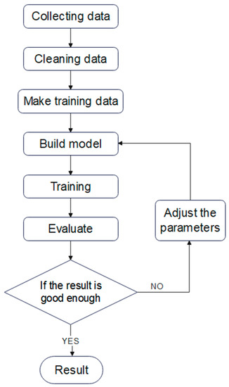
Figure 2. Neural-network model training process.

For the present research, the model parameters have been set differently from trial and error depending on the location as follows (Table 1):

Table 1. The adjusted parameters of the ANN model.

Parameter	Value or Function
η	0.0005
λ	Z-Score
L	Input + Hidden × 2 + Output
j	32, 32, 32
batch	32
ECHO (U, K, S) 1	300, 120, 130
Loss	MSE
optimizer	SGD
activation	sigmoid

¹ U:Unzen, K:Kuchinozu, S:Shimabara.

3. Results and Discussion

Once the model was trained and the results optimized using the SGD optimizer (Table 1), the results demonstrated that the prediction of rain gauge data from the XRain data is a good model fit, although it shows discrepancies depending on the station (Figure 3). At Unzen, the rain gauge model predicts a high peak of hourly rainfall > 10 mm successfully, but for smaller peaks, it tends to under-estimate the peaks between 5 mm and 10 mm hourly rainfalls (Figure 4).

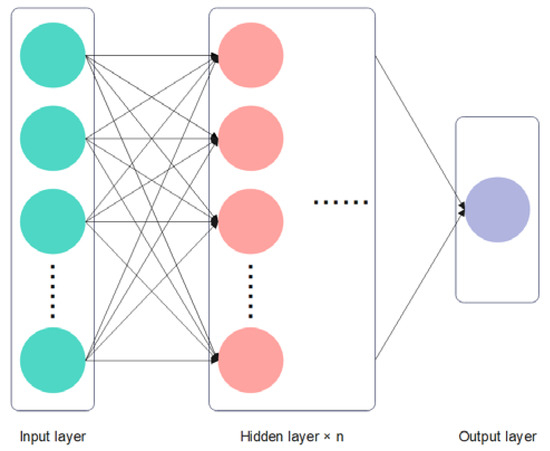
Figure 3. Conceptual diagram of BP neural network structure with the input layer, the hidden layer and the single output.

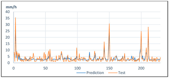
Figure 4. Predicted and modeled (test) results at Unzen Station.

At Kuchinozu station, the predictions and the test are of lower quality; neither the peaks nor the background rainfalls are well predicted, and this can certainly be attributed to the limited variability in the dataset, generating combinations that are two similar to one another if one wants to predict the changes (Figure 5).

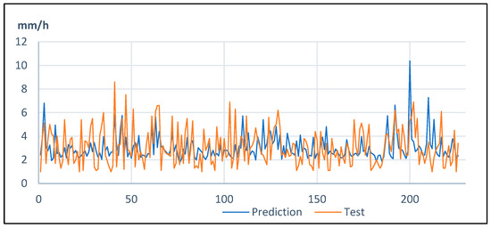
Figure 5. Predicted and modeled (test) results at Kuchinozu station.

Finally, at Shimabara station, peaks superior to 10 mm/h are well predicted, although the value is slightly underestimated. Peak rainfalls of 10 to 15 mm/h also show two occasions when the peak rainfalls were slightly overestimated (between the samples 200 and 250). The model also finds peak rainfalls between 5 and 10 mm/hour (Figure 6), but they are underestimated.

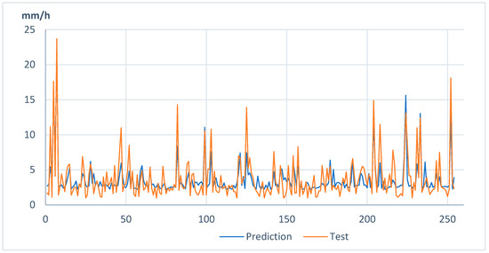
Figure 6. Predicted and modeled (test) results at Shimabara station.

To understand the importance of these errors: the error of the values of the rainfall against the test events shows that an hourly rainfall of 15 mm/h and higher are systematically underestimated. The worst estimate was for Mt. Unzen station when 35 mm/h was underestimated by 10 mm/h (Figure 7). The two other stations near sea level showed lower errors, with error values less than 4 mm for most values: only two values exceeded this error at Kuchinozu and a dozen at Shimabara station (Figure 8 and Figure 9). This issue emphasizes the necessity to separate the data of different seasons and from different wind directions in order to work on the topographic effects, which may affect the correspondence between the values of the XRAIN dataset and the rain gauge station.

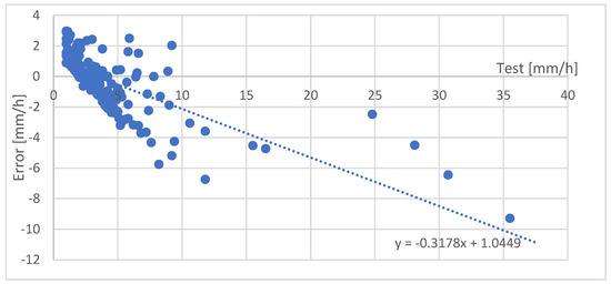
Figure 7. Errors at Unzen station.

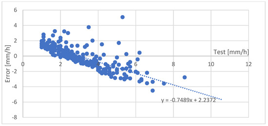
Figure 8. Errors at Kuchinozu station.

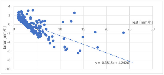
Figure 9. Errors at Shimabara station.

4. Conclusions

According to the results of the model calculation and error analysis, BP neural network can describe the relationship between rain gauge and spatial rainfall radar data to a certain extent. Additionally, the error of the model can be followed regularly. If the research continues in this direction, it is believed that it will be possible to calculate more accurate spatial rainfall data through rain gauges and other meteorological data.

References

- Gomez, C.; Lavigne, F.; Lespinasse, N.; Hadmoko, D.S.; Wassmer, P. Longitudinal structure of pyroclastic-flow deposits, revealed by GPR survey, at Merapi Volcano, Java, Indonesia. J. Volcanol. Geotherm. Res. 2008, 176, 439–447. [Google Scholar] [CrossRef]
- Gomez, C.; Lavigne, F.; Hadmoko, D.S.; Lespinasse, N.; Wassmer, P. Block-and-ash flow deposition: A conceptual model from a GPR survey on pyroclastic-flow deposits at Merapi Volcano, Indonesia. Geomorphology 2009, 110, 118–127. [Google Scholar] [CrossRef]
- Burgisser, A.; Bergantz, G.W. Reconciling pyroclastic flow and surge: The multiphase physics of pyroclastic density currents. Earth Planet. Sci. Lett. 2002, 202, 405–418. [Google Scholar] [CrossRef]
- Girolami, L.; Druit, T.H.; Roche, O. Towards a quantitative understanding of pyroclastic flows: Effects of expansion on the dynamics of laboratory fluidized granular flows. J. Volcanol. Getherm. Res. 2015, 296, 31–39. [Google Scholar] [CrossRef]
- Beget, J.; Gardner, C.; Davis, K. Volcanic tsunamis and prehistoric cultural transitions in Cook Inlet, Alaska. J. Volcanol. Geotherm. Res. 2008, 176, 377–386. [Google Scholar] [CrossRef]
- Lavigne, F.; Thouret, J.-C.; Voight, B.; Young, K.; LaHusen, R.; Marso, J.; Suwa, H.; Sumaryono, A.; Sayudi, D.S.; Dejean, M. Instrumental lahar monitoring at Merapi Volcano, Central Java, Indonesia. J. Volcanol. Geotherm. Res. 2000, 100, 457–478. [Google Scholar] [CrossRef]
- Lavigne, F.; Thouret, J.C.; Voight, B.; Suwa, H.; Sumaryono, A. Lahars at Merapi Volcano, Central Java: An overview. J. Volcanol. Geotherm. Res. 2000, 100, 423–456. [Google Scholar] [CrossRef]
- Starheim, C.A.; Gomez, C.; Davies, T.; Lavigne, F.; Wassmer, P. In-flow evolution of lahar deposits from video-imagery with implications for post-event deposit interpretation, Mount Semeru, Indonesia. J. Volcanol. Geotherm. Res. 2013, 256, 96–104. [Google Scholar] [CrossRef]
- Gomez, C.; Lavigne, F.; Hadmoko, D.S.; Wassmer, P. Insights into lahar deposition processes in the Curah Lengkong (Semeru Volcano, Indonesia) using photogrammetry-based geospatial analysis, near-surface geophysics and CFD modelling. J. Volcanol. Geotherm. Res. 2018, 353, 102–113. [Google Scholar] [CrossRef]
- Vazquez, R.; Capra, L.; Caballero, L.; Arambula-Mendoza, R.; Reyes-Davila, G. The anatomy of a lahar: Deciphering the 15th September 2012 lahar at Volcan de Colima, Mexico. J. Volcanol. Geotherm. Res. 2014, 272, 126–136. [Google Scholar] [CrossRef]
- Caballero, L.; Capra, L. The use of FLO2D numerical code in lahar hazard evaluation at Popocatepetl volcano: A 2001 lahar scenario. Nat. Hazards Earth Syst. Sci. 2014, 14, 3345–3355. [Google Scholar] [CrossRef]
- Pistolesi, M.; Cioni, R.; Rosi, M.; Aguilera, E. Lahar hazard assessment in the southern drainage system of Cotopaxi volcano, Ecuador: Results from multiscale lahar simulations. Geomorphology 2014, 207, 51–63. [Google Scholar] [CrossRef]
- De Belizal, E. Lahar-related impacts after the 2010 eruption of Merapi Volcano (Java, Indonesia). Geomorphol. Relief Process. Environ. 2013, 4, 463–480. [Google Scholar] [CrossRef]
- Gomez, C.; Lavigne, F. Transverse architecture of lahar terraces, inferred from radargrams: Preliminary results from Semeru Voclano, Indonesia. Earth Surf. Process. Landf. 2010, 35, 1116–1121. [Google Scholar] [CrossRef]
- Lavigne, F.; Tirel, A.; Le Floch, D.; Veryat-Charvillon, S. A real-time assessment of lahar dynamics and sediment load based on video-camera recording at Semeru Volcano, Inodnesia. In Debris-Flow Hazards Mitigation: Mechanics, Prediction, and Assessment; Rickenmann, D., Chenn, C., Eds.; Millpress Science Publishers: Rotterdam, The Netherlands, 2003; Volumes 1 and 2, pp. 871–882. [Google Scholar]
- Syarifuddin, M.; Hapsari, R.I.; Legono, D.; Oishi, S.; Mawanda, H.G.; Aisyah, N.; Shimomura, M.; Nakamichi, H.; Iguchi, M. Monitoring the rainfall intensity at two active volcanoes in Indonesia and Japan by small-compact X-band radars. IOP Earth Environ. Sci. 2020, 437, 012040. [Google Scholar] [CrossRef]
- Hapsari, R.I.; Oishi, S.; Syarifuddin, M.; Asmara, R.A.; Legono, D. X-MP Radar for Developing a Lahar Rainfall Threshold for the Merapi Volcano Using a Bayesian Approach. J. Disaster Res. 2019, 14, 811–828. [Google Scholar] [CrossRef]
- Nastos, P.T.; Moustris, K.P.; Larissi, I.K.; Paliatsos, A.G. Rain intensity forecast using Artificial Neural Networks in Athens, Greece. Atmos. Res. 2013, 119, 153–160. [Google Scholar] [CrossRef]
Disclaimer/Publisher’s Note: The statements, opinions and data contained in all publications are solely those of the individual author(s) and contributor(s) and not of MDPI and/or the editor(s). MDPI and/or the editor(s) disclaim responsibility for any injury to people or property resulting from any ideas, methods, instructions or products referred to in the content. |
© 2022 by the authors. Licensee MDPI, Basel, Switzerland. This article is an open access article distributed under the terms and conditions of the Creative Commons Attribution (CC BY) license (https://creativecommons.org/licenses/by/4.0/).