1. Introduction
A flow regime can be broadly categorized as perennial, intermittent, or ephemeral. In perennial systems there is a permanent connection between the stream and the groundwater, and good results can be obtained from rainfall–runoff models that do not explicitly represent the groundwater store. While ephemeral streams are defined as having short-lived flow after rainfall, intermittent streams become seasonally dry when the groundwater table drops below the elevation of the streambed during dry periods. A spatially intermittent stream may maintain flow over some sections, even during dry periods, due to locally elevated water tables.
Rainfall–runoff models often fail to simulate the hydrologic connection between streams and the groundwater system, where it tends to be variable in time and space, as is the case for spatially intermittent streams. This is the case for the Alcantara River basin in Sicily region (Italy), whose upstream is intermittent while its middle valley is characterized by perennial surface flows enriched by spring water arising from the big aquifer in the northern sector of the Etna volcano.
In a previous study, Aronica and Bonaccorso [
1] investigated the impact of future climate change on the hydrological regime of the Alcantara River basin by combining stochastic generators of daily rainfall and temperature with the IHACRES rainfall–runoff model under different climatic scenarios, to qualitatively investigate modifications to the hydropower potential. In their study, some simplifications to the system configuration have been considered to disregard the contribution of the groundwater component, as the emphasis was on simulating surface runoff only.
In the present study, a modified IHACRES rainfall–runoff model is proposed to better describe the complex connection between Northern Etna groundwater system and the Alcantara River basin. The modeling approach adopted in the present study involved separate but coordinated analysis of linearity and nonlinearity in the catchment response to rainfall, through a representation of catchment hydrological responses into serial linear and nonlinear modules. In particular, a modified version of IHACRES rainfall–runoff model, whose inputs are continuous series of concurrent daily streamflow, rainfall, and temperature data, was calibrated and validated at one of the main cross sections of the Alcantara River basin, where daily streamflow data are available. The structure of the model also provides the opportunity for dealing with the uncertainty of parameters when they are very short and poor-quality data series are available for model calibration and validation (Wagener et al. [
2]).
2. Model Description
The IHACRES model (acronym of “Identification of unit Hydrograph and Component flows from Rainfall, Evapotranspiration and Streamflow”) is a simple model designed to perform the identification of hydrographs and component flows purely from rainfall, evaporation, and streamflow data.
2.1. The IHACRES Model
In the original version of IHACRES, originally described by Jakeman et al. (1990) [
3], the rainfall–runoff processes are represented by two modules (see
Figure 1): a nonlinear loss module that transforms precipitation to effective rainfall considering the influence of the temperature, followed by a linear module based on the classical convolution between effective rainfall and the unit hydrograph to derive the streamflow.
In the literature, several studies on IHACRES development and application (Jakeman et al. 1990 [
3], 1993a [
4], 1993b [
5], 1994a [
6], 1994b [
7]; Jakeman and Hornberger 1993 [
8], Ye et al. 1997 [
9]) have demonstrated the following advantages and capabilities:
It is simple, parametrically efficient, and statistically rigorous;
Input data only consist of daily or monthly precipitation, temperature, and streamflow series;
The model provides a unique identification of system response even after a few years of input data;
The model efficiently describes the dynamic response characteristics of catchments;
The model allows researchers to obtain time series of interflow runoff with over-day storage, runoff from seasonal aquifers, and catchment wetness index;
The model can be run on any size of catchment;
Simulations are quick and computational demand is low.
2.2. The Modified IHACRES Model
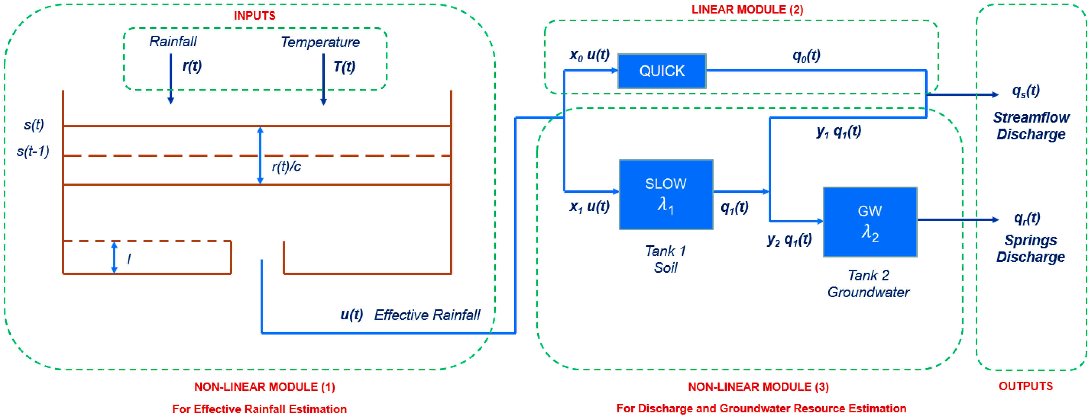
Hereafter, a modified version of the above-described IHACRES model is presented, which is better able to simulate the groundwater component of an aquifer system.
The structure of the modified IHACRES model shown in
Figure 2, which includes three modules: (1) a nonlinear loss module that transforms precipitation to effective rainfall by considering the influence of temperature and, after this, (2) a linear module based on the classical convolution between effective rainfall and the unit hydrograph able to simulate the quick component of the runoff, and (3) another nonlinear module that simulates the slow component of the runoff that feeds the groundwater storage. From the sum of the quick and the slow components (except for groundwater losses that represent the aquifer recharge) the total streamflow is derived. The need for this further nonlinear module (3) arises from the necessity to properly describe the groundwater component of the aquifer system and to model and quantify spring discharges.
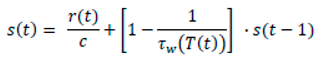
The nonlinear loss module (1) involves the calculation of an index of catchment storage
s(t) based upon an exponentially decreasing weighting of precipitation and temperature conditions:
where
s(
t) is the catchment storage index, or catchment wetness/soil moisture index at time t, varying between 0 and 1,
τw(
T(
t)) is a time constant which is inversely related to the declining temperature rate,
τ0 is the value of
τw(
T(
t)) for a reference temperature fixed to a nominal value depending on the climate and usually equal to 20 °C for warmer climates (Jakeman et al. 1994a [
6]),
c (mm) is a conceptual total storage volume chosen to constrain the volume of effective rainfall to equal runoff,
f [1/°C] is a temperature modulation factor. The effective rainfall
u(
t) is calculated as the product of total rainfall
r(
t) and the storage index
s(
t), taking into account the two parameters
p (an exponent of a power law used to describe the nonlinearity) and
l (that represents a threshold parameter) introduced by Ye et al. (1998) [
10] for low-yielding catchments, in order to better describe the strong nonlinearity caused by the impact of long dry periods on the soil surface:
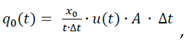
The effective rainfall feeds the two components of the outflow: the quick component (t) in the linear module (2) and the slow component (t) in the nonlinear module (3) that represents the soil response, conceptualized as a reservoir with storage constant λ1.
The quick and slow components, respectively, are represented as
with
where
x0 and
x1 represent the two share-out parameters of the effective rainfall
u(t).The sum of the quick component
q0(
t) calculated by the linear module and an aliquot of the slow component
y1q1 (t), gives as results the
streamflow discharge qs(
t):
The other aliquot
y2q1 (
t) of the slow component, instead, feeds the reservoir that represents groundwater with storage constant
λ2. The output of the groundwater reservoir is (
t) that represents
spring discharges is
with
3. Case Study
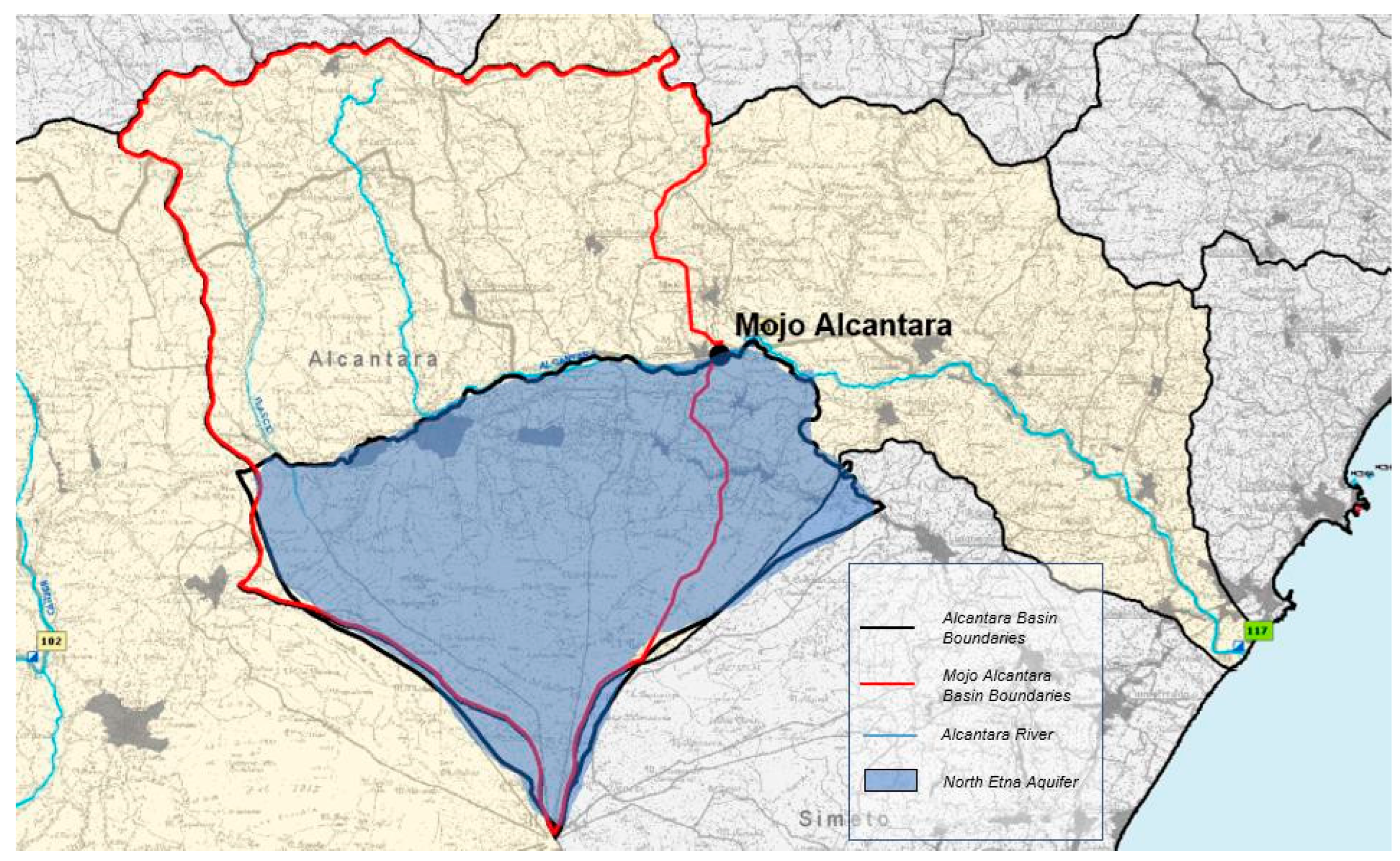
In the presented work, the above-described model has been applied to the Alcantara River basin that is located in north-eastern Sicily (the largest Italian island), encompassing the north side of Etna Mountain, the tallest active volcano in Europe. The river basin has an extension of about 603 km2. The headwater of the river is at 1400 m a.s.l. in the Nebrodi Mountains, while the outlet in the Ionian Sea is reached after 50 km (
Figure 3).
The mountain area on the right-hand side of the river is characterized by volcanic rocks with a very high infiltration capacity. Here, precipitation and snow melting supply a big aquifer whose groundwater springs are located at mid/downstream of the river, mixing with surface water and also contributing to feeding the river flow during the dry season. The left side of the basin is characterized by sedimentary soils and provides a seasonal contribution to the river flow as it follows the annual rainfall variability typical of a Mediterranean climate.
Groundwater resources are mainly used to supply all the municipalities located within the river catchment through local aqueducts, as well as small towns along the Ionian coast; in addition, the Alcantara River also supplies some industries, farms, and two hydroelectric power plants. This area is also regarded as a beautiful environmental reserve.
4. Calibration and Validation of the Model
The modified IHACRES rainfall–runoff model that is described above has a total number of 11 parameters, of which 5 parameters are in the effective rainfall estimation module (τ0, f, c, l, p) and 6 in the discharge estimation module (x0, x1, y1, y2, λ1, λ2), and only 9 needed to be calibrated.
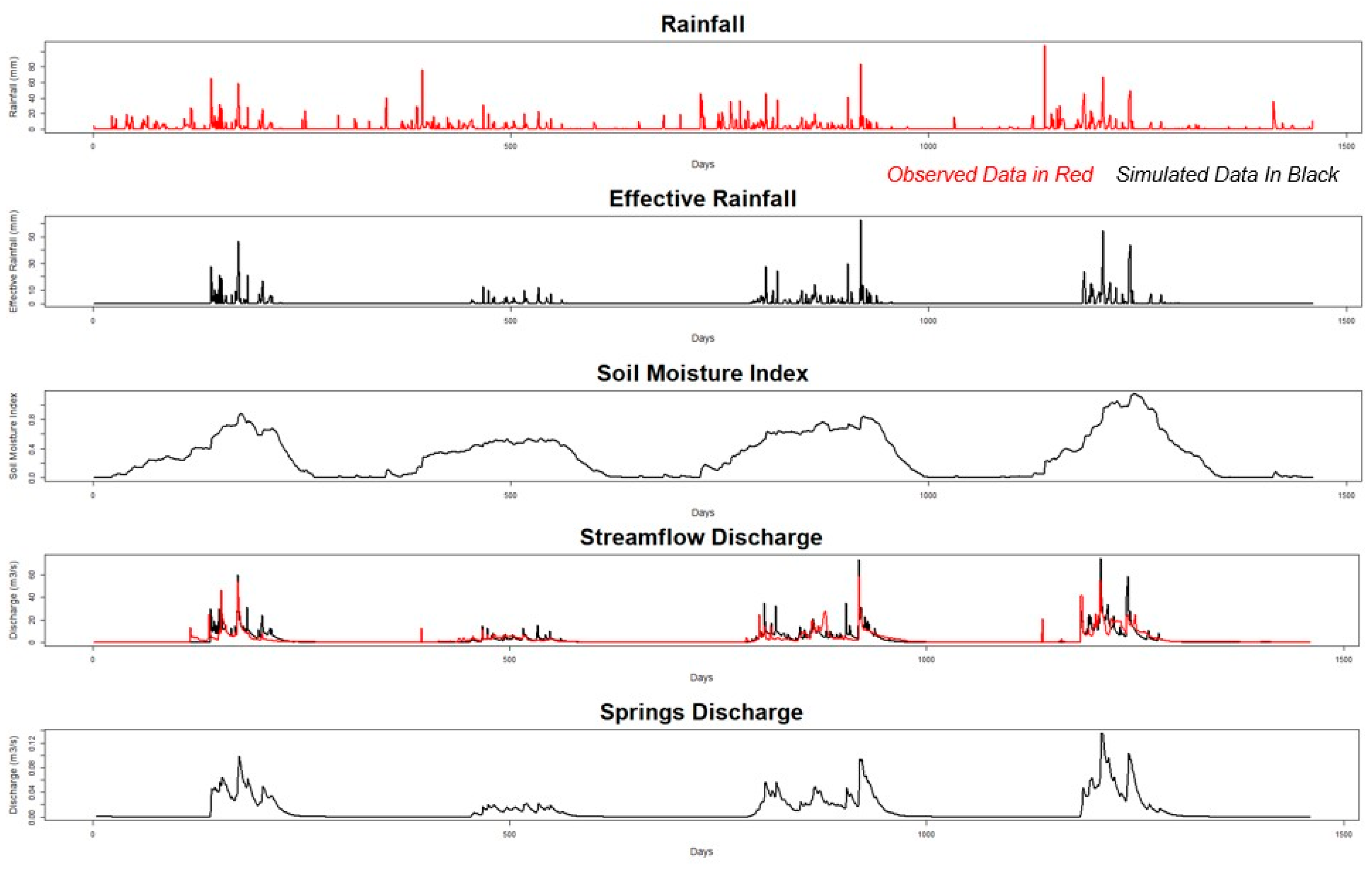
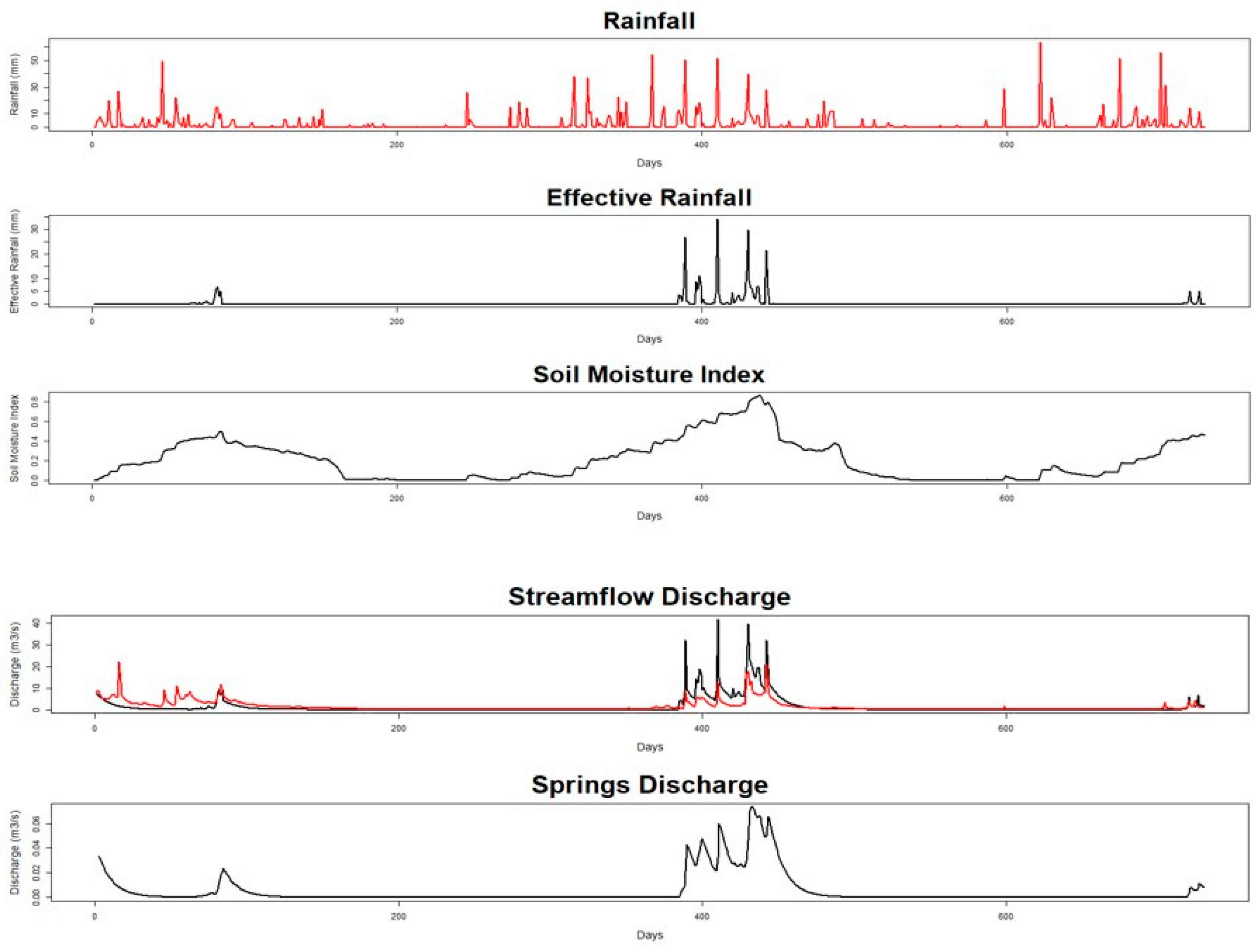
The input data used for running the model are daily point rainfall and temperature data spatially averaged over the considered area. The model has been calibrated on a 4-year daily streamflow discharge time series (1984–1986) at Mojo Alcantara hydrometric station (
Figure 3,
Table 1).
For this case study, there were no spring discharge time series available, therefore, to work around this issue, a priori condition was used as part of the calibration process, i.e., the mean annual aquifer recharge value simulated into the model has to be similar to the mean annual aquifer recharge value estimated in other studies (Sogesid, Piano di Tutela delle Acque Sicilia—PTA, Palermo 2007), that is, about 115 Mm3/year. Model calibration was carried out in R-Studio Software using the packages “
DEoptim” and “
hydroGOF”. In
Figure 4, results of the calibration are shown.
For the validation of the model, the daily streamflow discharge time series was observed at Mojo Alcantara hydrometric station during the period 1987–1988 (
Figure 5).
Moriasi et al. 2007 [
11] and Rittler et al. 2013 [
12] suggested that the efficiency of a hydrological model can be considered satisfactory when the Nash–Sutcliffe efficiency value of validation is between 0.50 and 0.65. Performance indicators are shown in
Table 2.
5. Conclusions and Future Perspectives
A hydrological conceptual rainfall–runoff model has been proposed to simulate the stream–aquifer interactions of the Alcantara River basin at Mojo cross-section in Sicily (Italy). The proposed modeling approach involves a compound analysis of linearity and nonlinearity in the catchment response to rainfall through serial combination of linear and nonlinear modules.
The novelty of this modified IHACRES model lies in the fact that the groundwater component and its interaction with surface water through spring discharges are modeled through a nonlinear module whose equations involve the calibration of four parameters easy to interpret.
Results have shown that the developed model is able to properly reproduce the seasonality in the hydrological response of the aquifer system in combination with the main streamflow. In particular, the results of model validation can be considered satisfactory since Nash–Sutcliffe efficiency value is close to the optimal range, as suggested in the literature by Ritter et al. 2013 [
11].
Further research will address the uncertainty and sensitivity analysis associated with the model and its parameters. More specifically, a first order sensitivity analysis should be carried out, to better understand the influence of parameters on the performance of the model, together with an uncertainty analysis based on the PLUE (profiled likelihood uncertainty estimation) approach.


