Quantification of a Ball-Speed Generating Mechanism of Baseball Pitching Using IMUs ^†

Abstract

The purpose of this study was to propose a methodology which quantifies the ball-speed generating mechanism of baseball pitching with the use of inertial measurement units (IMUs). IMUs were attached to the upper trunk, upper arm, forearm, and hand segments. The initial orientation parameters of each segment were identified using the differential iteration method from the acceleration and angular velocity of the sensor coordinate system output by IMUs attached to each segment. The motion of each segment was calculated and the dynamic contributions were then calculated. The motion of a baseball pitcher, who was instructed to throw at the target, was measured with a motion capture (mocap) system and IMUs. The results show that quantitative analysis of the ball-speed generation mechanism by the proposed method is almost similar to that conducted by the mocap system. In the future, this method will be employed to evaluate the ball-speed generation mechanism outside controlled laboratory conditions in an effort to help understand and improve the player’s motion.

1. Introduction

The capability to throw a high-speed fast ball is a crucial factor of a good pitcher in baseball games. Previous studies have shown that the motion-dependent term (MDT), consisting of centrifugal forces and the Coriolis force of the multi-link system, significantly contributes to the generation of ball speed in baseball pitching [1,2,3]. The large contribution of the MDT, which is sometimes called the “whip-like” effect, has been quantified with respect to motion data measured with a motion capture (mocap) system and high-speed camera system. Knowledge of the ball-speed generating mechanism can lead to a good understanding of pitching motion from the perspective of performance enhancement and injury prevention. Although high-speed camera systems and the mocap system are commonly used for the measurements of 3-D coordinate data of points on the body during sports motions, a huge amount of time and high cost are required to implement analyses of the motion. In contrast, previous studies have indicated that inertial sensors, which are small in size and weight, would be powerful alternative tools for the measurement and analysis of sports motions, despite the fact that the outputs of inertial measurement units (IMUs) are values expressed not in the world coordinate system, but in the sensor coordinate system [4,5]. Therefore, orientation of the sensor coordinate system is required when segment orientation is used for the reconstruction of body motions from output signals.

The purpose of this study was to propose a methodology which quantifies the ball-speed generating mechanism of pitching motion with the use of IMUs, in order to quantify the ball-speed generating mechanism without the use of an expensive mocap system in the field of baseball.

2. Methods

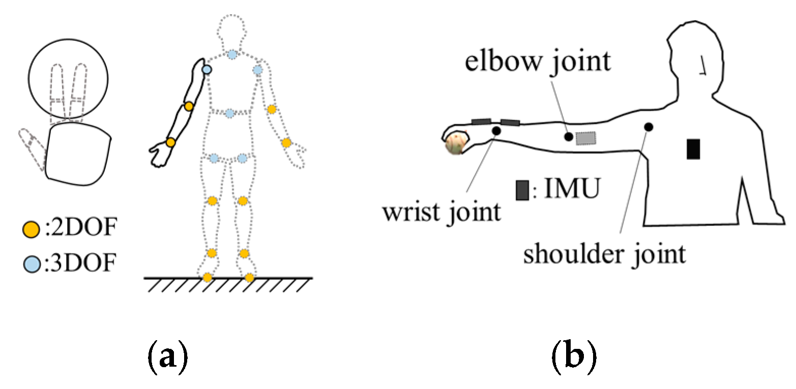
2.1. Data Collection

A right-handed experienced male baseball pitcher who was instructed to pitch a fast ball toward the target 18 m away participated in this study. Written informed consent was given prior to their participation, and approval for the experiment was obtained from the institution’s ethics committee. Three-dimensional coordinate data of sphere/semi-sphere markers which were attached to the whole body, IMUs, and the ball (e.g., body: 47 markers; four IMUs: 4 markers per unit; ball: 6 markers) during pitching motions were captured with a mocap system (VICON-MX, Vicon Motion Systems, UK, 14 cameras, 500 Hz). Simultaneously, the linear accelerations and angular velocities of the four segments (e.g., upper trunk, upper arm, forearm, and hand with a ball) on which IMUs were fixed with elastic tape during the pitching motion were measured with four IMUs (Figure 1b; e.g., 16 G/1500 dps $\times$ 1200 G/6000 dps $\times$ 3, DSP wireless motion sensors, 1000 Hz, Sport Sensing Co., Ltd., Fukuoka, Japan).

2.2. Dynamical Model of Upper Limb Segments with a Ball

The ball-side upper limb was modeled as a linked multi-segment system consisting of the upper arm, the forearm, and the hand with a ball. The rigid link model and the locations of the IMUs attached to the segments are shown in Figure 1a,b. Anatomical constraint axes (e.g., varus/valgus axis at the elbow joint; internal/external rotation axis at the wrist joint), along which the joints could not rotate freely, were considered [6]. Since the ball was assumed to be fixed to the hand segment coordinate system during the pitching motion, the hand and ball were assumed to be one rigid segment in this study.

2.3. Reconstructing Motion Data Using IMU Output Signals

When an IMU is attached to the body, the IMU’s output signals (e.g., tri-axial linear acceleration and angular velocity values) are expressed in the sensor coordinate system, because an IMU contains internal sensors (e.g., accelerometers and gyroscopes); thus, the initial position/orientation of each segment at the start of the motion is unknown. Therefore, in this study, using the fact that each segment of the body is connected by a joint, a relationship between accelerations was derived from IMU outputs (e.g., linear acceleration and angular velocity vectors), and the initial orientation parameters of the individual segments were then identified through a differential iteration method associated with IMU outputs of adjacent segments. Furthermore, the posture information of each segment in motion was calculated by using the identified initial orientation parameters and the angular velocity outputs of the IMU under the condition that the length from the origin of the IMU on each segment to each joint was known.

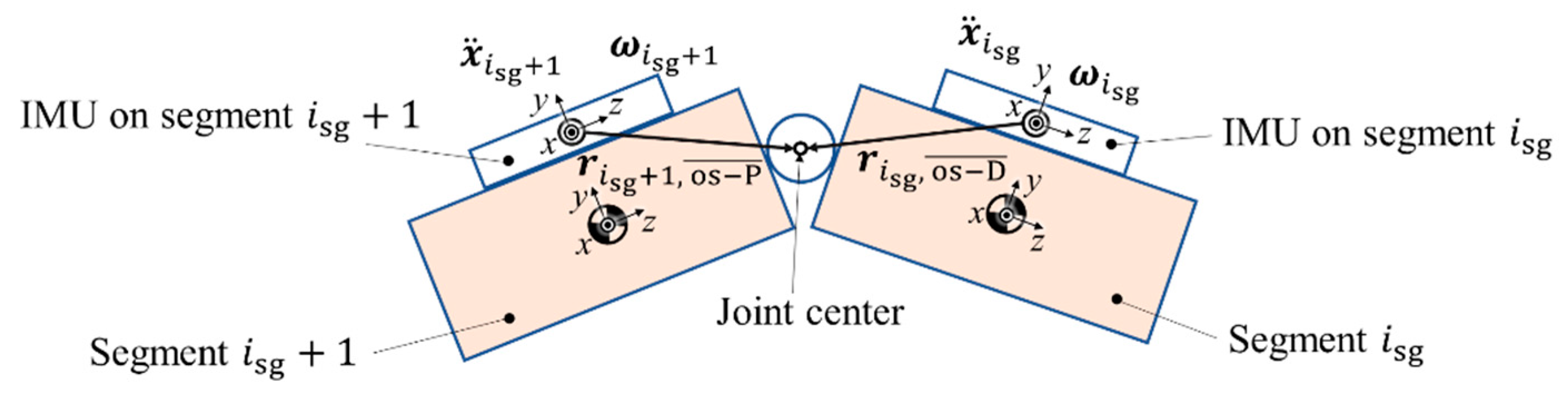
2.3.1. Geometric Constraint Relationships between IMUs’ Sensor Outputs

Assuming that every segment, on which each IMU is fixed, is connected to its adjacent segment at a joint (Figure 2), the geometric constraint for linked segments can be expressed as

$${}_{}{}^0\mathit{x}{}_{i+1}+{}_{}{}^0\mathit{r}{}_{i+1,\overline{\mathrm{os}-\mathrm{P}}}-{}_{}{}^0\mathit{x}{}_i-{}_{}{}^0\mathit{r}{}_{i,\overline{\mathrm{os}-\mathrm{D}}}={\mathit{O}}_{3\times 1},$$

(1)

where ${\mathit{O}}_{3\times 1}$ is a zero matrix with three rows and one column, and the vectors with barred subscripts os-D and os-P represent the position vectors from the origin of the IMU to the segment’s distal and proximal ends, respectively.

Double differentiating Equation (1) with respect to time yields a constraint equation in terms of acceleration of the joint center point:

$$\begin{gathered} {}_{}{}^0\ddot{\mathit{x}}{}_{i_{\mathrm{Sg}}+1}\left(k\right)+{}_{}{}^0\dot{\mathit{\omega }}{}_{i_{\mathrm{Sg}}+1}\left(k\right)\times {}_{}{}^0\mathit{r}{}_{i_{\mathrm{Sg}}+1,\overline{\mathrm{os}-\mathrm{P}}}+{}_{}{}^0\mathit{\omega }{}_{i_{\mathrm{Sg}}+1}\left(k\right)\times \left({}_{}{}^0\mathit{\omega }{}_{i_{\mathrm{Sg}}+1}\left(k\right)\times {}_{}{}^0\mathit{r}{}_{i_{\mathrm{Sg}}+1,\overline{\mathrm{os}-\mathrm{P}}}\right) \\ -{}_{}{}^0\ddot{\mathit{x}}{}_{i_{\mathrm{Sg}}}\left(k\right)-{}_{}{}^0\dot{\mathit{\omega }}{}_{i_{\mathrm{Sg}}}\left(k\right)\times {}_{}{}^0\mathit{r}{}_{i_{\mathrm{Sg}},\overline{\mathrm{os}-\mathrm{D}}}-{}_{}{}^0\mathit{\omega }{}_{i_{\mathrm{Sg}}}\left(k\right)\times \left({}_{}{}^0\mathit{\omega }{}_{i_{\mathrm{Sg}}}\left(k\right)\times {}_{}{}^0\mathit{r}{}_{i_{\mathrm{Sg}},\overline{\mathrm{os}-\mathrm{D}}}\right)={\mathit{O}}_{3\times 1}, \end{gathered}$$

(2)

where vectors ${}_{}{}^0\dot{\mathit{x}}{}_{i_{\mathrm{Sg}}+1}\left(k\right)$ and ${}_{}{}^0\mathit{\omega }{}_{i_{\mathrm{Sg}}+1}\left(k\right)$ denote the linear and angular velocity vector of the i_Sg-th segment expressed in the world coordinate system, respectively.

The orientation of the i_Sg-th segment at the time instant k can be expressed as a multiplication of two rotation matrices denoting segments’ orientations, as shown in the following equation:

$$\begin{array}{c}{}_{}{}^0\mathit{R}{}_{i_{\mathrm{Sg}}}\left(k\right)={}_{}{}^0\mathit{R}{}_{i_{\mathrm{Sg}}}\left(0\right){\mathsf{\Delta }\mathit{R}}_{i_{\mathrm{Sg}}}\left(k\right)\end{array},$$

(3)

where the orientation matrices ${}_{}{}^0\mathit{R}{}_{i_{\mathrm{Sg}}}\left(0\right)$ and ${\mathsf{\Delta }\mathit{R}}_{i_{\mathrm{Sg}}}\left(k\right)$ denote the initial orientation matrix at the start of analysis and the matrix showing change of the orientation of the segment from the start of the analysis, respectively, and the matrix denoting the change of the orientation can be expressed as

$${\mathsf{\Delta }\mathit{R}}_{i_{\mathrm{Sg}}}\left(k\right)={{\displaystyle \prod }}_{t=1}^k{\mathsf{\delta }\mathit{R}}_{i_{\mathrm{Sg}}}\left(t\right),$$

(4)

where the difference of orientation $\delta {\mathit{R}}_{i_{\mathrm{Sg}}}\left(k\right)$ caused by the angular velocity vector $\omega$ within a duration of $\mathsf{\Delta }t$ can be expressed through Rodrigues’ rotation formula by using the normalized angular velocity vector $\mathit{\omega }$.

Since the initial orientation parameter vector $\mathit{p}$ consisting of the roll-pitch-yaw angles of the adjacent segments is unknown in applications in fields, the nominal parameter vector $\tilde{\mathit{p}}$ was used at the initial condition.

When the nominal parameter vector coincides with the true values, the difference between two acceleration vectors at joint center points written by the following equation (Equation (5)) becomes small, and we can modify the nominal parameter vector $\tilde{\mathit{p}}$ so that the following equation ${\mathit{e}}_a\left(k,\tilde{\mathit{p}}\right)$ is ${\mathit{O}}_{3\times 1}$ through a differential iteration method with respect to the following equation:

$${\mathit{e}}_a\left(k,\tilde{\mathit{p}}\right)={\mathit{f}}_{\left(k\right)}\left(\tilde{\mathit{p}}\right)={}_{}{}^0\overline{\mathit{R}}{}_{i_{\mathrm{Sg}}+1}\left({\tilde{\mathit{p}}}_{i_{\mathrm{Sg}}}\right)\Delta {\mathit{R}}_{i_{\mathrm{Sg}}+1}\left(k\right)a_{i_{\mathrm{Sg}}+1}\left(k\right)-{}_{}{}^0\overline{\mathit{R}}{}_{i_{\mathrm{Sg}}}\left({\tilde{\mathit{p}}}_{i_{\mathrm{Sg}}}\right)\Delta {\mathit{R}}_{i_{\mathrm{Sg}}}\left(k\right)a_{i_{\mathrm{Sg}}}\left(k\right)$$

(5)

$${\mathit{a}}_{i_{\mathrm{Sg}}}\left(k\right)={}_{}{}^{i_{\mathrm{Sg}}}\ddot{\mathit{x}}{}_{i_{\mathrm{Sg}}}\left(k\right)+{}_{}{}^{i_{\mathrm{Sg}}}\dot{\mathit{\omega }}{}_{i_{\mathrm{Sg}}}\left(k\right)\times {}_{}{}^{i_{\mathrm{Sg}}}\mathit{r}{}_{i_{\mathrm{Sg}},\overline{\mathrm{os}-\mathit{P}}}+{}_{}{}^{i_{\mathrm{Sg}}}\mathit{\omega }{}_{i_{\mathrm{Sg}}}\left(k\right)\times \left({}_{}{}^{i_{\mathrm{Sg}}}\mathit{\omega }{}_{i_{\mathrm{Sg}}}\left(k\right)\times {}_{}{}^{i_{\mathrm{Sg}}}\mathit{r}{}_{i_{\mathrm{Sg}}+1,\overline{\mathrm{os}-\mathit{P}}}\right),$$

(6)

where the acceleration vector ${\mathit{a}}_{i_{\mathrm{Sg}}}\left(k\right)$ is obtained from the sensor outputs of linear acceleration ${}_{}{}^{i_{\mathrm{Sg}}}\ddot{\mathit{x}}{}_{i_{\mathrm{Sg}}}\left(k\right)$and the angular velocity vector ${}_{}{}^{i_{\mathrm{Sg}}}\mathit{\omega }{}_{i_{\mathrm{Sg}}}\left(k\right)$ from the IMUs fixed on the segments i_Sg+1 and i_Sg. The angular acceleration vector ${}_{}{}^{i_{\mathrm{Sg}}}\dot{\mathit{\omega }}{}_{i_{\mathrm{Sg}}}\left(k\right)$was calculated numerically from the differentiation of ${}_{}{}^{i_{\mathrm{Sg}}}\mathit{\omega }{}_{i_{\mathrm{Sg}}}\left(k\right)$ with respect to time.

In the case that the initial orientation parameter vector shows true values, the following equation would be satisfied:

$${}_{}{}^0\mathit{R}{}_{i_{\mathrm{Sg}}+1}\left(0\right)\Delta {\mathit{R}}_{i_{\mathrm{Sg}}+1}\left(k\right){\tilde{\mathit{a}}}_{i_{\mathrm{Sg}}+1}\left(k\right)-{}_{}{}^0\mathit{R}{}_{i_{\mathrm{Sg}}}\left(0\right)\Delta {\mathit{R}}_{i_{\mathrm{Sg}}}\left(k\right){\tilde{\mathit{a}}}_{i_{\mathrm{Sg}}}\left(k\right)={\mathit{O}}_{3\times 1},$$

(7)

where the rotation matrix ${}_{}{}^O\mathit{R}{}_{i_{\mathrm{Sg}}}\left(0\right)$ is given by the multiplication of three rotation matrices ${}_{}{}^0\mathit{R}{}_{i_{\mathrm{Sg}},z}\left({\varphi }_{i_{\mathrm{Sg}}}\left(0\right)\right),{}_{}{}^0\mathit{R}{}_{i_{\mathrm{Sg}},y}\left({\theta }_{i_{\mathrm{Sg}}}\left(0\right)\right)$, and ${}_{}{}^0\mathit{R}{}_{i_{\mathrm{Sg}},x}\left({\psi }_{i_{\mathrm{Sg}}}\left(0\right)\right)$about the z, y, and x axes with roll, pitch, and yaw angles (e.g., ${\varphi }_{i_{\mathrm{Sg}}}\left(0\right)$, ${\theta }_{i_{\mathrm{Sg}}}\left(0\right)$, and ${\psi }_{i_{\mathrm{Sg}}}\left(0\right)$) at the time instant of the start of the analysis.

2.3.2. Parameter Identification of the Initial Orientation Matrix of Segments

If the initial orientation parameter vector $\mathit{p}$ shows true values of the segment orientation parameters, Equation (8) derived from Equation (5) is a zero vector. Therefore, a differential iteration method with respect to $\mathit{p}$ was conducted, in order to find the true values of initial orientation parameters which make Equation (8) a zero vector.

$${\mathit{e}}_{\mathit{a}}\left(k,\mathit{p}\right)=f_{\left(k\right)}\left(\mathit{p}\right)$$

(8)

The analytical form of the partial differentiation of Equation (8) is expressed by the following form:

$$\Delta {\mathit{e}}_{\mathit{a}}\left(\mathit{k},\mathit{p}\right)=\left[\begin{array}{cc}\frac{\mathbf{\partial }{\mathit{f}}_{\left(k\right)}\left(k,p\right)}{\mathbf{\partial }{\mathit{p}}_1}& \frac{\mathbf{\partial }\mathit{f}\left(\mathit{k},\mathit{p}\right)}{\mathbf{\partial }{\mathit{p}}_2}\end{array} \begin{array}{cc}\cdots & \frac{\mathbf{\partial }\mathit{f}\left(\mathit{k},\mathit{p}\right)}{\mathbf{\partial }{\mathit{p}}_6}\end{array}\right]\left[\begin{array}{c}\begin{array}{c}\Delta {\mathit{p}}_1\\ \Delta {\mathit{p}}_2\end{array}\\ ⋮\\ \Delta {\mathit{p}}_6\end{array}\right].$$

(9)

Instead of calculating the partial differentiation of Equation (9) analytically, the differentiation was calculated numerically by the following procedures.

Firstly, the difference between the value of Equation (9) under the nominal parameter, vector, in addition to one percent error in the nominal parameter, and the value of Equation (9) with the nominal parameter vector, was acquired. Secondly, the differences were divided by the one percent parameter value, in order to obtain the partial differentiation of Equation (9) numerically:

$$\frac{\partial {\mathit{f}}_{\left(k\right)}\left(k,\mathit{p}\right)}{\partial {\mathit{p}}_i}=\frac{\left\{{\mathit{e}}_{\mathit{a}}\left(k,\tilde{\mathit{p}}+\frac{\widetilde{{\mathit{p}}_i}}{100}\right)-\Delta {\mathit{e}}_{\mathit{a}}\left(k,\tilde{\mathit{p}}\right)\right\}}{\frac{\widetilde{{\mathit{p}}_i}}{100}},$$

(10)

$$\begin{gathered} \Delta {\mathit{e}}_{\mathit{a}}\left(k,\mathit{p}\right)={\mathit{A}}_k\Delta \mathit{p} \\ {\mathit{A}}_k=\left[ \begin{array}{cccc}{\mathit{A}}_{p_1, k}& {\mathit{A}}_{p_2,k}& \cdots & {\mathit{A}}_{p_6,k}\end{array}\right], {\mathit{A}}_{p_i, k}=\frac{\partial \mathit{f}\left(k,\mathit{p}\right) }{\partial p_i}. \end{gathered}$$

(11)

The initial orientation parameter of the segment was modified and renewed using $\Delta p$ in Equation (11), employing a pseudo inverse matrix as follows:

$$\Delta \mathit{p}={\mathit{A}}^{+}\Delta \mathit{a}, {\mathit{A}}^{+}={\left({\mathit{A}}^{\mathrm{T}}\mathit{A}\right)}^{-1}{\mathit{A}}^{\mathrm{T}},\mathit{A}=\left[\begin{array}{c}{\mathit{A}}_1\\ ⋮\\ {\mathit{A}}_{n_{{\mathrm{F}}_{\mathrm{r}}}}\end{array}\right],\Delta \mathit{a}=\left[\begin{array}{c}\Delta {\mathit{e}}_{\mathit{a}}\left(1,\mathit{p}\right)\\ ⋮\\ \Delta {\mathit{e}}_{\mathit{a}}\left(n_{{\mathrm{F}}_{\mathrm{r}}},\mathit{p}\right)\end{array}\right],$$

(12)

where the parameter vector was modified using the pseudo inverse matrix ${\mathit{A}}^{+}$of the matrix $\mathit{A}$ as

$${\mathit{p}}_{i_{\mathrm{IT}}}={\mathit{p}}_{i_{\mathrm{IT}}}+\beta \Delta {\mathit{p}}_{i_{\mathrm{IT}}}={\mathit{p}}_{i_{\mathrm{IT}}}+\beta {\mathit{A}}^{+}\Delta \mathit{a},$$

(13)

where $i_{\mathrm{IT}}$ indicates the iteration number of calculations for the differential iteration method searching modified initial orientation parameters. The modification of the initial orientation parameter was iterated until the norm of the joint center acceleration error vector $\Vert {\mathit{e}}_{\mathit{a}}\left(k,\mathit{p}\right) \Vert$displayed a small value (i.e., ${10}^{-1}\mathrm{m}/{\mathrm{s}}^2$).

2.4. Equation of Motion for the Body and Ball System

An analytical form of the equation of motion for the body with a ball system can be expressed as follows:

$$\stackrel{·}{\mathit{V}}={\mathit{A}}_{\mathit{T}\mathrm{a}}{\mathit{T}}_{\mathrm{act}}+{\bar{\mathit{A}}}_{\mathit{V}}\mathit{V}+{\mathit{A}}_{\mathit{G}}\mathit{G}+{\mathit{A}}_{\mathrm{err}},$$

(14)

where $\mathit{V}$ is the generalized velocity vector consisting of linear velocity vectors with respect to the center of gravity (CG) and angular velocity vectors for all segments; ${\mathit{A}}_{\mathit{T}\mathrm{a}}$ and ${\mathit{A}}_{\mathit{G}}$ indicate the coefficient matrices for the active joint torque vector $T_{\mathrm{act}}$ and gravitational force vector $\mathit{G},$ respectively; ${\bar{\mathit{A}}}_{\mathit{V}}\mathit{V}$ indicates the motion-dependent term (MDT) consisting of force and moment caused by centrifugal and Coriolis forces and the gyroscopic effective moment; and ${\mathit{A}}_{\mathrm{Err}}$ is the modeling error term consisting of the acceleration constraint term of the shoulder joint and fluctuation terms caused by segment lengths and anatomical constraint joint axes [1].

2.5. Contributions to the Ball Speed

After integrating Equation (14) with respect to time, the ball variables can be calculated as [1]

$$q_{\mathrm{ball}}={\mathit{S}}_{\mathrm{ball}}\mathit{V}, q_{\mathrm{ball}}={\dot{\mathit{x}}}_{\mathrm{ball}},$$

(15)

where the matrix S_ball denotes the transforming matrix from the generalized velocity vector to the ball CG velocity vector ${\dot{\mathit{x}}}_{\mathrm{ball}}$.

The dynamic contributions of the individual terms to the generation of the ball variables are shown as

$$q_{\mathrm{ball}}=C_{\mathrm{Trq}}+C_{\mathrm{MDT}}+C_{\mathrm{G}}+C_{\mathrm{Err}},$$

(16)

where the terms C_Trq, C_MDT, and C_G respectively denote the contributions of the joint torque term, the MDT, and the gravitational term, and the term C_Err is the contribution of modeling error term to the generation of ball velocity. For example, the contribution of the joint torque term is given as follows:

$$C_{\mathrm{Trq}}={\mathit{e}}_{\mathrm{ball}}^T{\mathit{S}}_{\mathrm{ball}}{{\displaystyle \int }}^{\text{}}{\mathit{A}}_{Ta}{\mathit{T}}_{\mathrm{act}}dt, {\mathit{e}}_{\mathrm{ball}}=\frac{{\dot{\mathit{x}}}_{\mathrm{ball}}}{\left|{\dot{\mathit{x}}}_{\mathrm{ball}}\right|}.$$

(17)

Furthermore, the MDT was converted to other terms using the same method as in a previous study [1].

3. Results and Discussions

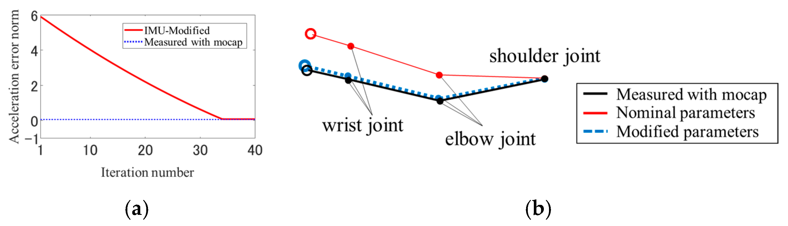
3.1. Iterative Calculation in Parameter Identification

Figure 3a,b show the results of parameter identification of the initial orientation matrix of the segment. The norm value of the acceleration error in Equation (8) converges to the norm value measured with mocap by iterative calculation (Figure 3a). The identified initial orientation parameters in the coronal plane approached the orientation measured with mocap (Figure 3b).

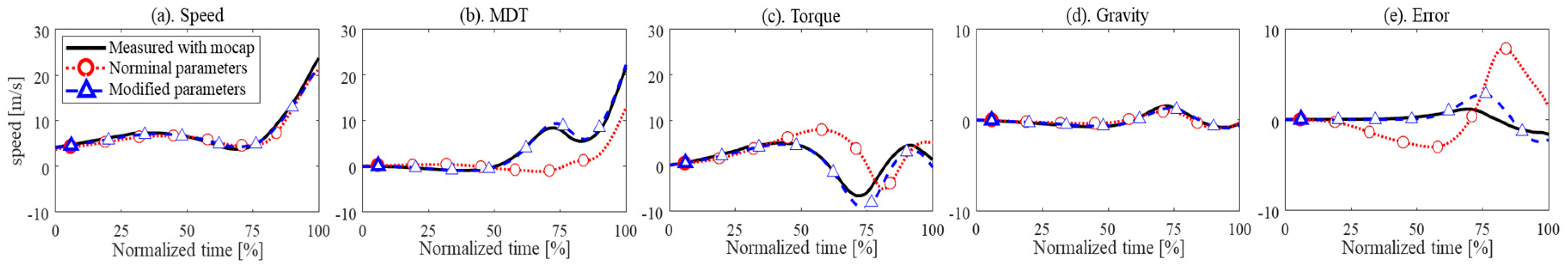
3.2. Contributions to the Ball Speed

Figure 4 shows the contributions of the individual terms to the ball speed with respect to the three types of motion data: (i) data obtained with the mocap system, (ii) data constructed from IMU-output signals using modified (identified) initial orientation parameters, and (iii) data constructed from IMU-output signals using nominal initial orientation parameters. Since the contributions of individual terms to the ball speed with respect to the data constructed using the identified initial orientation parameters were similar to the contributions calculated from the mocap information (Figure 4), the ball-speed generating mechanism can be quantified by using IMUs. Similar to the results of a previous study [1], the MDT is the largest contributor to the ball speed prior to ball release. Although detailed results are omitted due to space restrictions, the contributions of individual joint torques to the generation of the ball speed when considering the generating factor of the MDT for the data constructed with the identified initial orientation parameters were similar to the contributions calculated from the data measured with a motion capture system. Since errors of segments’ orientation still remain during pitching motions due to the wobbling of IMUs on the soft tissue relative to the humerus, errors of the upper arm segment exist between the motions being constructed from modified IMU outputs and mocap marker position outputs.

4. Conclusions

This study has proposed a method which realizes quantification of the ball-speed generating mechanism of baseball pitching motions by using inertial measurement units. Identifying the initial orientation parameters through a differential iteration method derived from the geometric constraint equations associated with the accelerations of joint center points using signal outputs (e.g., acceleration and angular velocities expressed in the sensor coordinate system) from IMUs attached to each segment enables the movements of individual segments to be constructed. Induced speed analyses were conducted and investigated for the constructed motion data and motion-capture data. The results indicate that the quantitative analysis of the proposed method, in terms of the ball-speed generation mechanism, is similar to that of a mocap system. In the future, this method will be employed to evaluate the ball velocity generating mechanism outside controlled laboratory conditions and will help to understand and improve the player’s pitching motion. Furthermore, by applying this method to the quantification method of the generating mechanism of the constraint torque, such as the valgus/varus axial torque at the elbow joint using the induced constraint torque analysis based on a dynamic equation, the risk of injury can be evaluated quantitatively.

References

1. Koike, S.; Uzawa, H.; Hirayama, D. Generation mechanism of linear and angular ball velocity in baseball pitching. Procedia Eng. 2018, 2, 206. [Google Scholar]
2. Naito, K.; Maruyama, T. Contributions of the muscular torques and motion-dependent torques to generate rapid extension during overhand baseball pitching. Procedia Eng. 2008, 11, 47–56. [Google Scholar] [CrossRef]
3. Hirashima, M.; Yamane, K.; Nakamura, Y.; Ohtsuki, T. Kinetic chain of over arm throwing in terms of joint rotations revealed by induced acceleration analysis. J. Biomech. 2008, 41, 2874–2883. [Google Scholar] [CrossRef] [PubMed]
4. Berkson, E.; Aylward, R.; Zachazewski, J.; Paradiso, J.; Gill, T. IMU Arrays: The biomechanics of baseball pitching. Orthop. J. Harv. Med. Sch. 2006, 8, 90–94. [Google Scholar]
5. Roetenberg, D.; Luinge, H.; Slycke, P. Xsens MVN: Full 6DOF Human Motion Tracking Using Miniature Inertial Sensors; Xsens Technologies B.V.: Enschede, The Netherlands, 2009. [Google Scholar]
6. Koike, S.; Ishikawa, T.; Willmott, A.P.; Bezodis, N.E. Direct and indirect effects of joint torque inputs during an induced speed analysis of a swinging motion. J. Biomech. 2019, 86, 8–16. [Google Scholar] [CrossRef] [PubMed]
Figure 1. A schematic representation of (a) a model of the upper limb with the ball, and (b) initial configuration of the participant during the pitching motion in experiments. (a) Upper limb model; (b) the locations of inertial measurement units (IMUs) on the segments and initial configuration at the start of the pitching motion.
Proceedings 49 00057 g001
Figure 2. A schematic representation of two adjacent rigid segments connecetd via a joint.
Proceedings 49 00057 g002
Figure 3. (a) Acceleration error norm due to the values measured with mocap and the output value of the IMU by repeated calculation at the wrist joint; (b) initial orientation stick picture of the values measured with mocap, IMU-nominal, and IMU-modified in the coronal plane.
Proceedings 49 00057 g003
Figure 4. Time curves of the contributions of individual terms to the ball speed, where the titles in Figure 4a,c are as follows; speed: measured ball speed; torque: total contribution of joint torque terms.
Proceedings 49 00057 g004
Publisher’s Note: MDPI stays neutral with regard to jurisdictional claims in published maps and institutional affiliations.