An Analysis of the Use of Multiple Transmission Power Levels on Wireless Sensor Networks ^†

Abstract

The energy consumption in wireless sensor networks is the critical concern of different studies, especially because of the great effort, or even the impossibility, to replace the battery of their motes. Consequently, it is fundamental to investigate and evaluate the energy spent by every individual task executed by the motes in order to provide an efficient use of their batteries. In this work, we employ different metrics to present a thorough study of how the use of multiple transmission power levels affects multihop wireless sensor networks. This work is motivated by the current employment of the multiple transmission power levels, on both academic works and commercial solutions, which is a novel feature of some radio transceivers commonly used in wireless sensor network motes. Aiming for reliable and extensive analysis, this study employs simulations in different scenarios and models of commonly employed electronic components. The contribution of this works is a detailed investigation of the impact caused by the use of different transmission power levels employing different metrics, offering a wide perspective on the subject. In general, the results of this study indicate that the use of multiple power levels grants both positive and negative results, according to the scenario and metrics analyzed.

1. Introduction

The electronic industry is regularly lowering the power consumption of their products, achieving even figures of nanowatts [1]. The problem is that that even a small but continuous consumption can deplete a battery, which usually is the primary power supply of a mote, in the long-term. As studied in [2,3], there can be scenarios where a large amount of the energy budget is still available, even after the end of the operational lifetime of the network, indicating an opportunity to a more efficient operation.

Recent research works [4,5] and commercial devices [6,7] use dynamic transmission power levels in order to achieve different goals. In this work, we investigate the use of multiple transmission power levels on wireless sensor networks in different scenarios and analyze its impact using various metrics in order to provide useful study about the subject.

2. Related Works and Methodology

Similar to [8], this work employed simulations using energy consumption data acquired from both direct measurements [8,9] and the datasheets of the electronic components. The Mathematical models and the related works are referenced along with this section (for further details, consider referring to their respective literature review).

2.1. Mote Architecture

The motes considered in this work’s analysis follow a basic architecture [8,10], having: one battery (a 150 mAh COMP-18-3-NMH); one microcontroller (Atmel Atmega8L [11]); one radio transceiver (Digi XBee PRO [7]); and one sensor (Texas Instruments LM75 [12]).

2.2. Energy Consumption

The energy consumption model adopted in this work considers the summation of the energy spent by each part [8,10,13]. As shown in their datasheets [7,11,12], all parts have different consumption levels according to their operational states. Consequently, these different consumptions were computed in our simulations.

2.3. Primary and Secondary Energy Consumption

We classify the energy consumption into two categories: Primary and Secondary. Primary energy consumption refers to the energy consumed by active states, like reading sensors, processing data, transmitting or receiving messages, etc. Secondary energy consumption refers to the energy consumed by inactive states, like idle and power-down/sleep states [7,11,12].

It is important to note that every electronic part used in a mote consumes energy, including when they are in secondary states, like idle and sleep and that the energy consumption of secondary states is usually very low when compared to the primary states [9].

2.4. Transmission Power Levels

The transmission power levels were calculated using the Plane Earth Propagation Model [8,14] with the path loss exponent set to 3.5. In order to produce a relevant analysis, six different transmission power level scenarios were evaluated: (i) transmission power for reaching one hop; (ii) transmission power for reaching two hops; (iii) transmission power for reaching three hops; (iv) transmission power for reaching four hops; (v) transmission power for reaching five hops; and (vi) transmission power for directly reaching the base station.

As all motes transmit their messages towards a single base station, their maximum transmission power did not exceed the power needed to reach the base station in any situation.

2.5. Network Lifetime

As stated in [15], the network lifetime of a wireless sensor network can have different definitions. In this work, we define the lifetime of a wireless sensor network as the period of time from the moment the network operation begins until the first mote runs out of battery [8].

2.6. Network Cost

We define the network cost as the summation of the price of all parts used in the simulated networks. The quotation of all components (see Section 2.1) was made in 2018 and their average prices are considered in this work. The total cost of the network considered in this work, with 10 motes, is US$445.10.

2.7. Message Log

After the end of each simulation, all messages were accounted and divided into four categories:

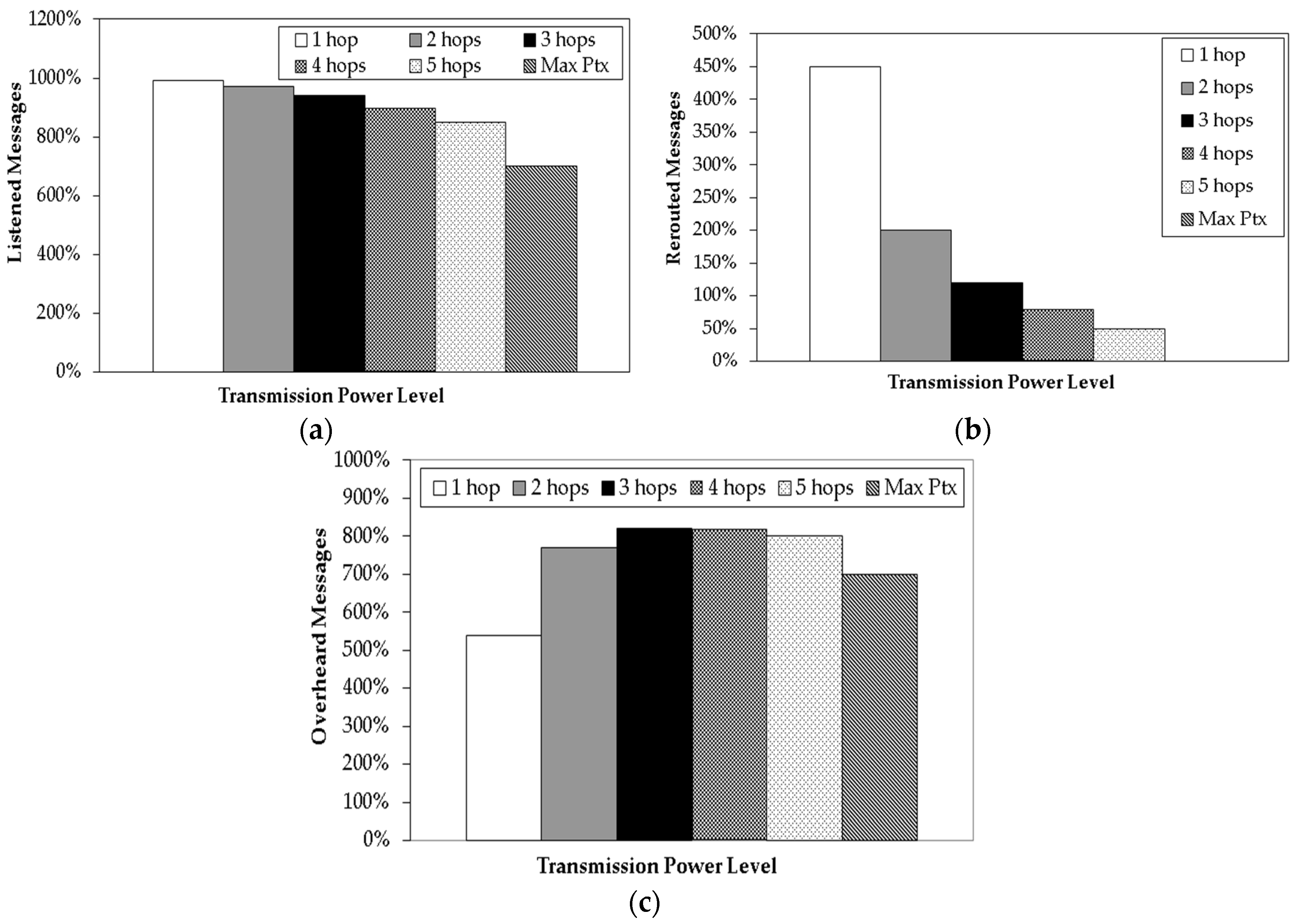
• Listened Messages: All messages received by a mote, regardless their addressee.
• Rerouted Messages: All messages that a mote had to reroute in order to reach the base station.
• Overheard Messages: Only the messages that a mote received but were not addressed to it.
• Generated Messages: All messages created and transmitted by a mote.

3. Simulations and Results

All simulations used identical parts/motes and network topology, with 10 motes organized in a row, with the base station allocated in its extremity, as shown in Figure 1. The networks simulated in this work followed the rules of a time-driven network [8,16], therefore, all motes performed their tasks following a network cycle. All motes kept their microcontrollers, sensors, and radio transceivers on the power-down/sleep states until the moment when they had to sense the environment and transmit their messages or to receive or to reroute messages of other motes. As the addressee of a message is only known after receiving and processing a message, we also considered the promiscuous reception [17].

As the motes were equipped with 540 Coulomb batteries (150 mAh), the maximum lifetime of the simulated motes (i.e., when the mote neither sends nor receives messages) would be 7142.85 h.

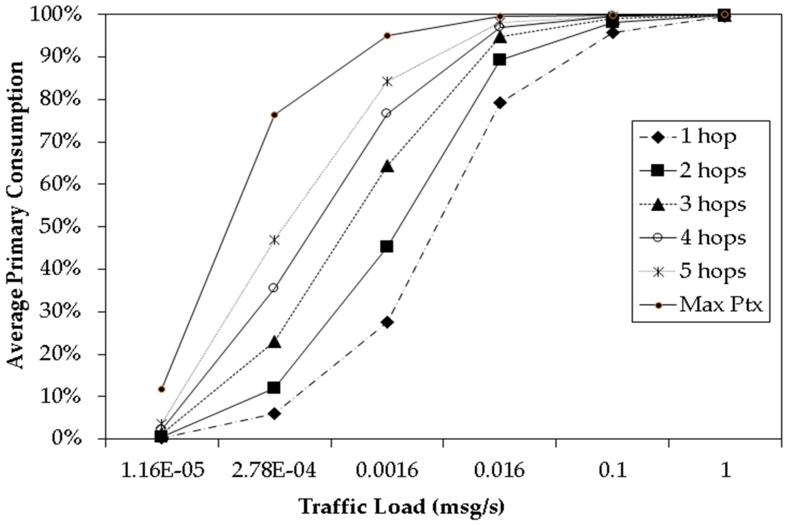
3.1. Primary and Secondary Consumption

As can be observed in Figure 2, the average primary consumption, which is the consumption for reading sensors, transmitting, receiving, and processing messages, has a decreasing share on the total consumption of the network when the message generation is lower. This trend was maintained with all power levels.

3.2. Energy Consumption Profile

The transmission power increase also had an impact on the energy consumption profile of the simulated networks. As can be observed in

Table 1. Energy consumption of each part/functionality.

Transmission Power/Reach	Radio-Tx	Radio-Rx	Microcontroller	Sensor
1 hop	32.03%	24.70%	41.18%	2.08%
2 hops	77.47%	11.18%	10.38%	0.96%
3 hops	91.11%	4.96%	3.48%	0.44%
4 hops	95.57%	2.61%	1.56%	0.24%
5 hops	97.52%	1.52%	0.80%	0.15%
Base station	99.47%	0.34%	0.14%	0.04%

, due to the transmission power increase, the energy spent on transmissions (labeled as “Radio-TX”) increased, following the transmission power increase. The energy consumption profile of secondary states is shown in

Table 2. Energy consumption profile of secondary states in all scenarios.

Radio	Microcontroller	Sensor
47.61%	23.81%	28.58%

.

3.3. Lifetime

Table 3. Lifetime of the simulated networks with different transmission powers.

Traffic Load (msg/s)	Lifetime (in Hours)—1 hop	Lifetime (in Hours)—2 hops	Lifetime (in Hours)—3 hops	Lifetime (in Hours)—4 hops	Lifetime (in Hours)—5 hops	Lifetime (in Hours)—Max Power
1.16 x 10−5	7111.35	7067.55	6981.56	6863.59	6568.67	4797.62
2.78 x 10−4	6457.86	5690.14	4595.49	3614.01	2307.02	561.01
0.00166	4364.89	2821.47	1651.28	1041.33	526.16	100.01
0.166	969.93	437.78	208.51	119.86	56.35	10.13
0.1	182.28	76.89	35.62	20.26	9.45	1.69
1	18.65	7.76	3.57	2.10	0.94	0.17

shows that the lifetimes of the simulated networks with higher transmission power were shorter when compared to standard transmission power. It can also be noted that the difference between the lifetime of the simulated networks decreased when the traffic load got lower. As the traffic load was reduced, networks using higher transmission power almost attained the same lifetime of the standard transmission power network (1 hop), with an exception on the network using the maximum transmission power.

3.4. Network Cost per Working Hour

Table 4. Network cost per hour of the simulated networks with different transmission powers.

Traffic Load (msg/s)	Network Cost Per Hour—1 Hop	Network Cost Per Hour—2 Hops	Network Cost Per Hour—3 Hops	Network Cost Per Hour—4 Hops	Network Cost Per Hour—5 Hops	Network Cost Per Hour—Max Power
1.16 x 10−5	US$0.06	US$0.06	US$0.06	US$0.06	US$0.07	US$0.09
2.78 x 10−4	US$0.06	US$0.07	US$0.10	US$0.12	US$0.19	US$0.79
0.00166	US$0.10	US$0.16	US$0.27	US$0.42	US$0.84	US$4.45
0.166	US$0.46	US$1.01	US$2.13	US$3.71	US$7.90	US$43.94
0.1	US$2.44	US$5.79	US$12.49	US$21.97	US$47.10	US$263.37
1	US$23.86	US$57.36	US$124.68	US$211.95	US$473.51	US$2618.23

shows the cost of each network per hour of their lifetime. As the network cost is the same on all simulated networks (US$445.10), the lifetime was critical, making the cost of each network cheaper according to the decreasing traffic generation. In this scenario, all network costs got lower when the traffic generation was reduced.

3.5. Message Log

Figure 3a shows that the total of listened messages in relation to generated messages (see Section 2.7) decreased with higher transmission power, from 990% to 770%.

Figure 3b shows that the total of rerouted messages in relation to generated messages decreased with higher transmission power, from 450% to 0%.

Figure 3c shows that the total of overheard messages in relation to generated messages increased with higher transmission power, from 540% to 700%, with peaks of 820%.

4. Conclusion

The use of multiple transmission power levels achieved both positive and negative results, depending on the employed metric. The results about the traffic of messages were very positive, but it cannot be analyzed alone, without energy issues, due to the focus of this work on wireless sensor networks. As the messages were sent further when using higher transmissions power levels, the quantity of rerouted messages also decreased. One result that can be inferred, but is not analyzed in this work, is that the less hops a message has to perform, the lower is the chance of it be corrupted or lost.

The lifetime and network cost had very negative results when using short generation periods, but on networks with longer generation periods, the difference between the lifetimes of the simulated was considerably reduced. These similar lifetimes of low traffic networks can be understood by analyzing the ratio between their primary and secondary energy consumption. As the primary energy consumption is caused by tasks related to active tasks, like reading sensors and sending/receiving messages, its share is larger when the generation period is short and smaller when the generation period is long. The results indicate that the use of multiple transmission power levels would suit better in low message traffic networks or when dealing with reliability/message loss constraints.

References

1. Li, G.; Xu, Z.; Xiong, C.; Yang, C.; Zhang, S.; Chen, Y.; Xu, S. Energy-efficient wireless communications: Tutorial, survey, and open issues. IEEE Wirel. Commun. 2011, 18, 28–35. [Google Scholar] [CrossRef]
2. Lian, J.; Naik, K.; Agnew, G.B. Data capacity improvement of wireless sensor networks using non-uniform sensor distribution. Int. J. Distrib. Sens. Netw. 2006, 2, 121–145. [Google Scholar] [CrossRef]
3. Akyildiz, I.F.; Su, W.; Sankarasubramaniam, Y.; Cayirci, E. Wireless sensor networks: A survey. Comput. Netw. 2002, 38, 393–422. [Google Scholar] [CrossRef]
4. Gao, F.; Li, J.; Jiang, T.; Chen, W. Sensing and Recognition When Primary User Has Multiple Transmit Power Levels. IEEE Trans. Signal Process. 2015, 63, 2704–2717. [Google Scholar] [CrossRef]
5. Chen, Z.; Gao, F.; Zhang, X.; Li, J.C.F.; Lei, M. Sensing and Power Allocation for Cognitive Radio with Multiple Primary Transmit Powers. IEEE Wirel. Commun. Lett. 2013, 2, 319–322. [Google Scholar] [CrossRef]
6. Freescale Semiconductor Inc. Freescale MC13202 Datasheet with Addendum. Available online: https://www.nxp.com/docs/en/data-sheet/MC13202.pdf (accessed on 31 September 2018).
7. Digi International Inc. Digi XBee/XBee-PRO OEM RF Modules Product Manual. Available online: https://www.digi.com/resources/documentation/digidocs/pdfs/90000976.pdf (accessed on 31 September 2018).
8. Miranda, F.A.M.; Cardieri, P. The impact of multiple power levels on the lifetime of Wireless Sensor Networks. In Proceedings of the 2016 IEEE International Symposium on Consumer Electronics (ISCE), São Paulo, Brazil, 20–30 September 2016; pp. 103–104. [Google Scholar]
9. Miranda, F.A.M.; Cardieri, P. Current Consumption in Radio Modules for Wireless Sensor Networks. In Proceedings of the XXXV Simpósio Brasileiro de Telecomunicações e Processamento de Sinais—SBrT2017, São Paulo, Brazil, 3–6 September 2017. [Google Scholar]
10. Vieira, M.A.M.; Coelho, C.N.; da Silva, D.C.; da Mata, J.M. Survey on wireless sensor network devices. In Proceedings of the IEEE Conference on Emerging Technologies and Factory Automation (EFTA 2003), Lisbon, Portugal, 16–19 September 2003; Proceedings (Cat. No.03TH8696). Volume 1, pp. 537–544. [Google Scholar]
11. Atmel Corporation. 8-bit Atmel with 8KBytes In-System Programmable Flash ATmega8 ATmega8L Manual. Available online: http://ww1.microchip.com/downloads/en/devicedoc/atmel-2486-8-bit-avr-microcontroller-atmega8_l_summary.pdf (accessed on 31 September 2018).
12. Maxim Integrated National Semiconductor LM75 Digital Temperature Sensor and Thermal Watchdog with Two—Wire Interface. 2009.
13. Girban, G.; Popa, M. A glance on WSN lifetime and relevant factors for energy consumption. In Proceedings of the 2010 International Joint Conference on Computational Cybernetics and Technical Informatics, Timisoara, Romania, 27–29 September 2010; pp. 523–528. [Google Scholar]
14. Rappaport, T.S. Wireless Communications: Principles and Practice, 2nd ed.; Prentice Hall: Upper Saddle River, NJ, USA, 2002. [Google Scholar]
15. Mak, N.H.; Seah, W.K.G. How Long is the Lifetime of a Wireless Sensor Network? In Proceedings of the International Conference on Advanced Information Networking and Applications, Bradford, UK, 26–29 May 2009; pp. 763–770. [Google Scholar]
16. Hodon, M.; Chovanec, M.; Cechovic, L.; Hudik, M.; Milanova, J.; Kochlan, M.; Jurecka, M.; Kapitulik, J.; Sevcik, P. Maximizing performance of low-power WSN node on the basis of event-driven-programming approach: Minimization of operational energy costs of WSN node control unit. In Proceedings of the IEEE Symposium on Computers and Communication (ISCC), Larnaca, Cyprus, 6–9 July 2015; pp. 204–209. [Google Scholar]
17. Feeney, L.M.; Nilsson, M. Investigating the energy consumption of a wireless network interface in an ad hoc networking environment. In Proceedings of the Twentieth Annual Joint Conference of the IEEE Computer and Communications Society (Cat. No.01CH37213), Anchorage, AK, USA, 22–26 April 2001; Volume 3, pp. 1548–1557. [Google Scholar]
Figure 1. Network simulated in this work.
Proceedings 04 00003 g001
Figure 2. Average primary/secondary energy consumption.
Proceedings 04 00003 g002
Figure 3. Message log of the simulated networks: (a) listened messages; (b) rerouted messages; (c) overheard messages.
Proceedings 04 00003 g003