2.1. Regional Calibration Procedure
Solar radiometry metrology has advanced considerably since 1970. Discussions of metrology of solar radiometry can be found in [
9,
10,
11,
12,
13,
14,
15,
16,
17]. The advances in metrology of solar radiometry have been driven by the requirements of more accurate determination of the TSI, (total solar irradiance) measured by orbiting satellites equipped with self calibrating cavity radiometers. Ground based measurements have benefitted from these advances, and in particular, the cavity radiometers calibrated by electrical substitution.
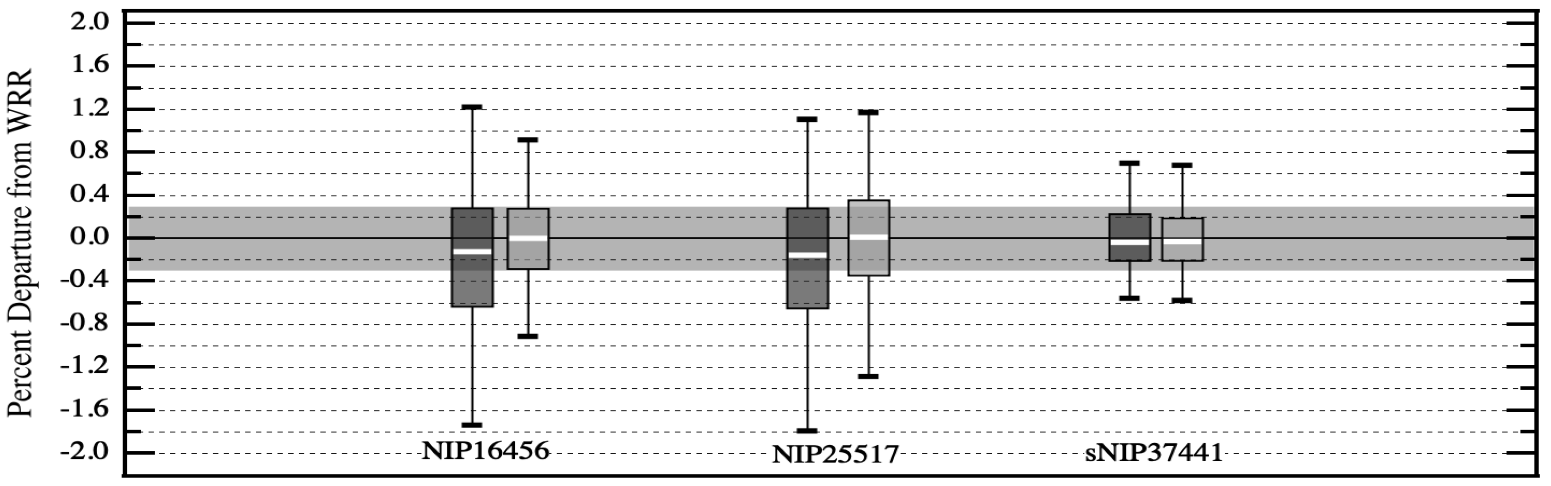
IPC participants with self calibrating cavity radiometers are in position to reproduce the precision achievable at an IPC. For example, in Region IV (North America, Central America and the Caribbean), an annual ad hoc pyrheliometer comparison is conducted at NREL (National Renewable Energy Laboratory) in Golden Colorado. These NPC (NREL Pyrheliometer Comparison) events are conducted every fall during non-IPC years. A surrogate WSG, based on a group of participating cavities from the most recent IPC, is used to create a reference irradiance scale. NPC participants unable to attend a recent IPC, can compare their cavities to this surrogate WSG and realize a precision of ratios comparable to those achievable at an IPC.
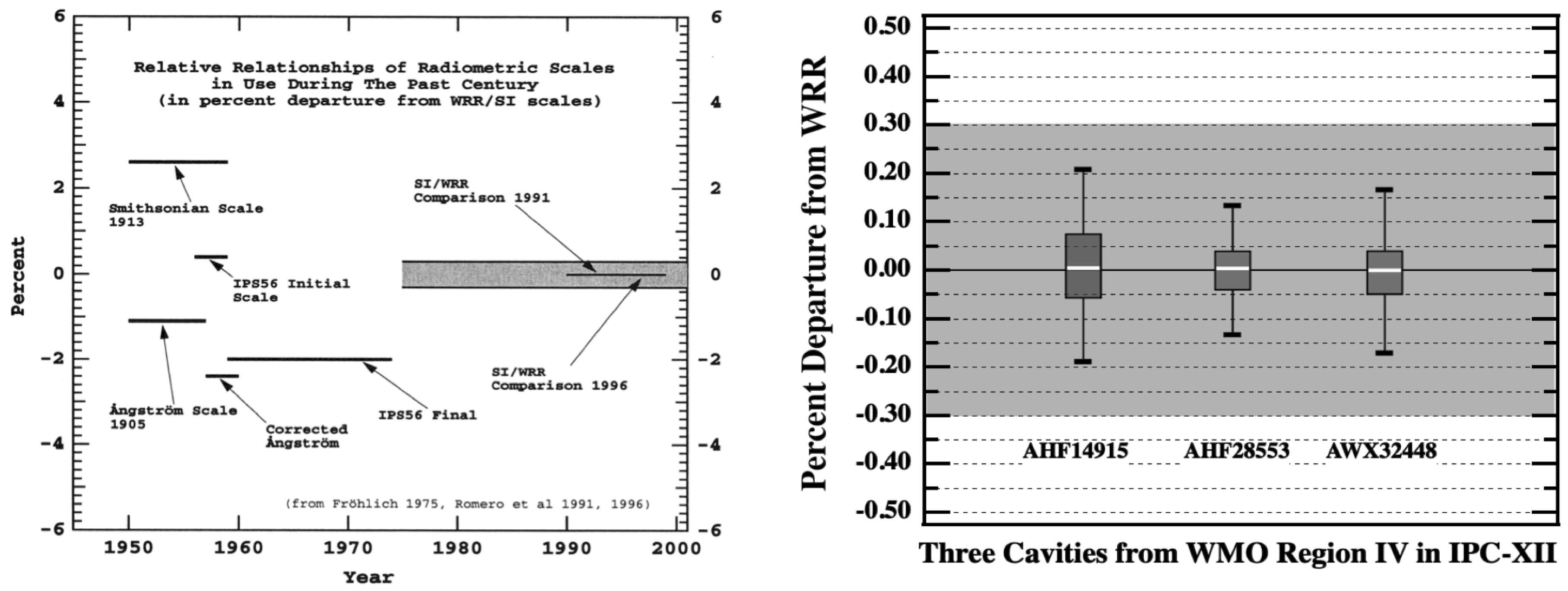
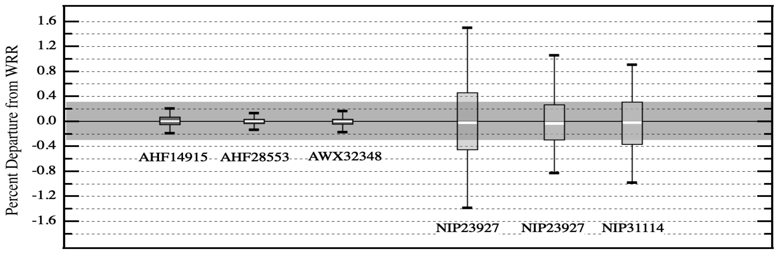
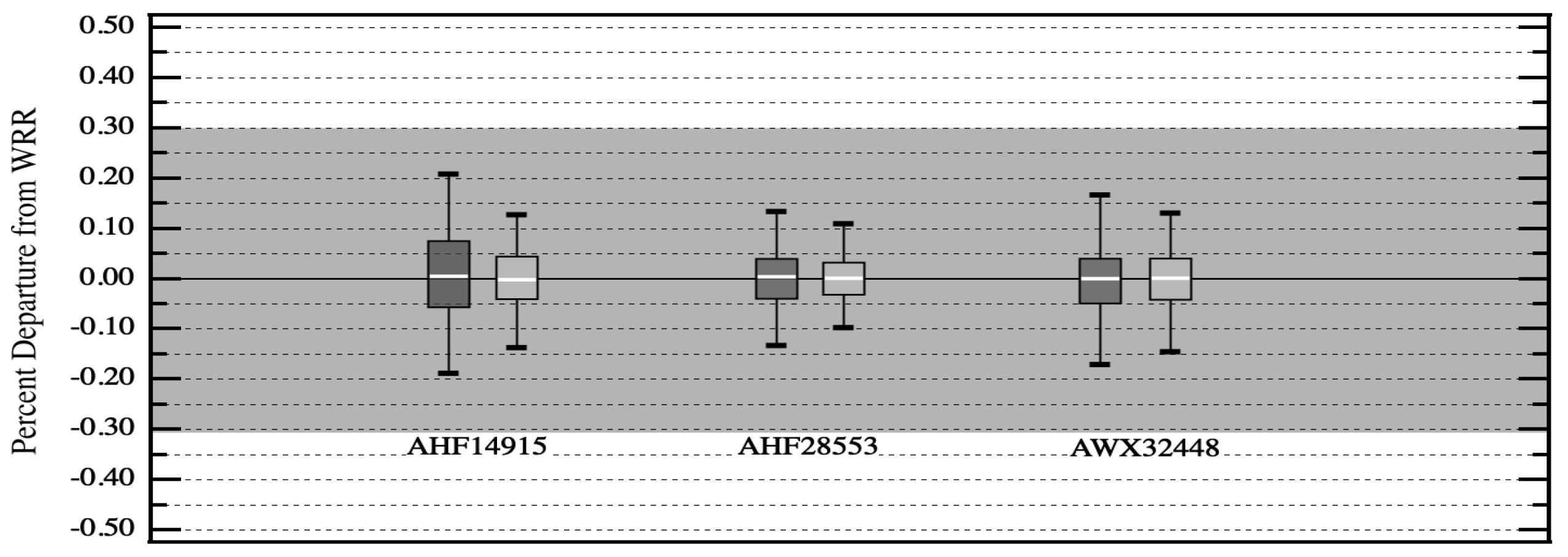
Figure 3 illustrates the precision of the same cavities displayed in
Figure 2, but for their results from an NPC conducted in 2018 at NREL [
18], three years after their most recent participation in IPC-XII. Cavities that participate in an NPC but not the most recent IPC are able to create their own surrogate WRR and establish traceability to the WSG/WRR in Davos.
A working class pyrheliometer at the regional level is usually calibrated by operating it side by side with a reference cavity traceable to the most recent IPC or NPC and calibrations can be performed on an as needed basis. Typically, a group of working class pyrheliometers are calibrated together using a WRR or NPC traceable cavity. A protocol similar to an IPC is used for collecting measurements of direct beam solar irradiance from the reference cavity and output voltages. Data are collected at chosen time intervals and the voltage readings from a pyrheliometer under test are ratioed to the concurrent reference cavity irradiance values. Unlike an IPC or NPC, the pyrheliometers under test are not self-calibrating. The ratios formed by dividing readings from the pyrheliometers under test by the irradiances measured with the cavity have units of microvolts per watt per square meter and are referred to as responsivities. These ratios are collected over time periods that can vary from hours to days and weeks, depending on frequency of clear sky conditions during the calibration period and the judgment of personnel performing the calibration. Orthodox statistical techniques are used to process the set of ratios from individual pyrheliometers and one ratio value is generated and assigned as its responsivity. The assigned ratio is the chosen model for transforming voltage readings from a working class pyrheliometer into irradiance values traceable to the surrogate WRR generated by the reference cavity. In various forms, depending on the history of pyrheliometer design, this has been the model for assigning a reference scale irradiance to a given output from a working class pyrheliometer and has been used for the past century. In contrast, a typical IPC lasts for three weeks and usually clear sky periods occur such that enough readings are recorded to confidently produce WRR correction factors for all participating instruments. Protocols for IPC comparisons impose strict constraints on when data is officially recorded for determination of WRR factors but the IPCs are only scheduled every five years. At the regional level, working class pyrheliometers are utilized in long term monitoring networks, renewable energy applications, efficiency monitoring of solar power generation sites, commercial calibration services and research institutions. These pyrheliometers may also be installed at remote field sites and operate unattended and continuously for months and years. Periodically they require recalibration and are replaced by a more recently calibrated unit. This is the reality of establishing and maintaining long term monitoring networks for measurement of solar radiation.
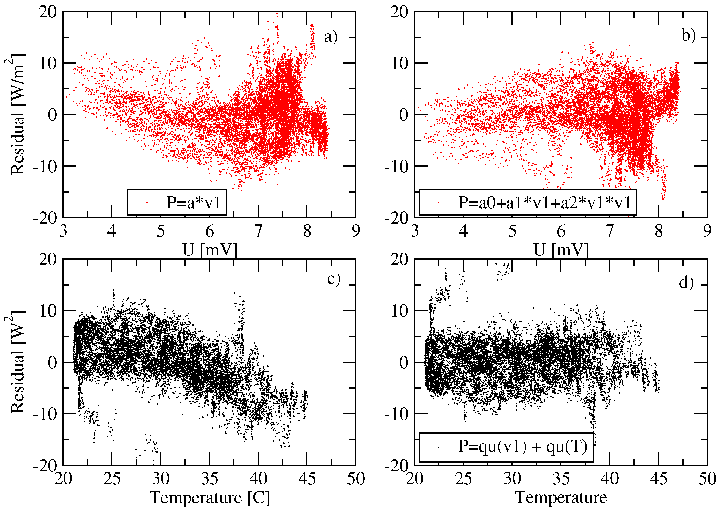
2.3. Multivariate Linear Regression
The preceding discussion results in three likely parameters for the model:
. However, the functional form of
f is unknown. Based on the experience of the change of the residuals using low order polynomials it appears reasonable to express the model function as a sum of multivariate monomials
where
E is the expansion order of the model. As basis sets we consider the set of all monomials in these variables up to a total degree (the sum of all three exponents
) of 3, corresponding to 20 different basis functions, for example monomials like
,
or
. Depending on the expansion order out of these 20 basis functions
E are chosen and used for a multivariate linear regression to the data. This yields for a given expansion order
possible models. Since a priori we neither know the most adequate expansion order
E nor the best set of monomials for a given expansion order we compute the model evidence in the MAP approximation for all possible combinations up to
, resulting in the comparison of more than
different models. Our approach employs standard Bayesian model comparison as outlined e.g., in [
19]. For the large number of models it is only possible because most of the necessary numerics to compute the evidence can be done analytically, as is shown next.
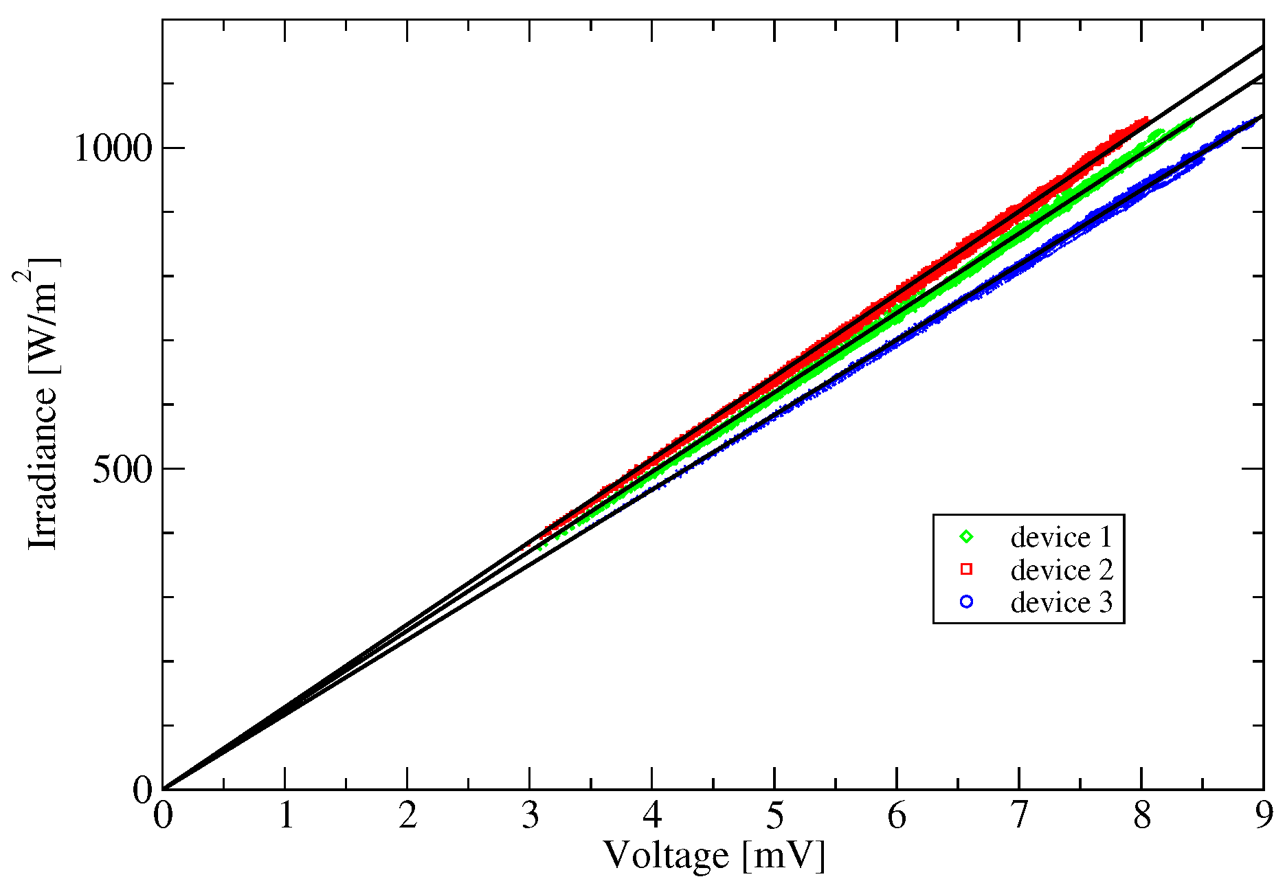
If we assume that
and
and negligible uncertainty in the voltage measurement the data
are given by
and the likelihood for
N independent measurements becomes
The notation simplifies if we introduce the vectors
and
and the matrices
and
in the argument
of the exponential. Then
It is convenient to introduce new variables
and
in the exponent, resulting in
The maximum of the likelihood is achieved for
In the following, we assume that the inverse of the matrix
exists. A necessary condition is
, i.e., we have at least as many measurements as there are parameters. If the inverse matrix exists then
Since
is quadratic in
we can rewrite
in Equation (
4) as a complete square in
plus a residue
This form is achieved via a Taylor expansion about
. The second derivatives (Hessian) provide
The matrix on the right-hand-side also shows up in the maximum likelihood solution
The residue
R in Equation (
5) is the constant
of the Taylor expansion, that can be transformed into
This general result can be cast in an advantageous form employing singular value decomposition [
20] of the matrix
:
The sizes of the matrices
,
, and
are
,
, and
respectively. The transposed matrix
is simply
and the product
becomes, using the unitarity of
The last equation is also known as the spectral decomposition of the real symmetric matrix
. We assume that the singular values are strictly positive, in order that the inverse of
exists. The virtue of the spectral decomposition is that it yields immediately the inverse
as
It is easily verified that the matrix product of Equations (
11),
12 yields the identity matrix
, which is a consequence of the left unitarity of
. The maximum likelihood estimate
is given by
where
(
) are the column vectors of
(
). The maximum likelihood estimate
is thereby expanded in the basis
with expansion coefficients
.
We now turn to the Bayesian estimation of
[
19]. The full information on the parameters
is contained in the posterior distribution
from which we can determine for example the maximum posteriori (MAP) solution via
For a sufficient number of well determined data the likelihood is strongly peaked around its maximum
, while the prior will be comparatively flat, in particular if it is chosen uninformative. A reliable approximate solution will then be obtained from
which is the maximum likelihood estimate. Similar arguments hold for posterior expectation values of any function
For general
the integrals can only be performed numerically. Using the fact that the likelihood is generally precisely localized compared to the diffuse prior. This suggests, that we replace the prior
by
and take it out of the integrals
Now, since
is a multivariate Gaussian in
the expectation value
and the covariance
can easily be determined
We have derived a reasonable approximation for the normalization
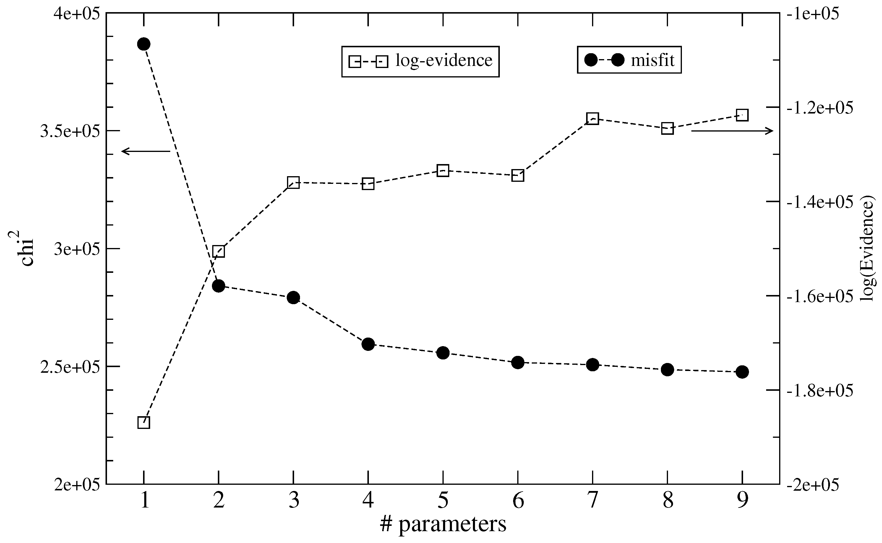
Z, also called the »prior predictive value« or the »evidence«.
Z represents the probability for the data, given the assumed model. The question at hand in the present problem is of course whether the data require really a high expansion order
E or are they also satisfactorily explained by some lower order
. For these problems the full expression for
Z is required including the prior factor. The remaining Gaussian integral in Equation (18) can be performed easily resulting in
The singular value decomposition of the argument of the exponential yields
and the evidence finally reads
The exponent in Equation (
21) represents that part in the data that is due to noise or a different model.
It remains to assign a prior distribution to the linear parameters
of the model. For simplicity we assign a normalized uniform prior for all components
in the range
and
outside. Thus each additional parameter reduces the log-evidence by
. More refined prior distributions based on Maximum Entropy concepts are possible [
19] but have not been considered in this work. The standard deviation of the power measurements was assumed to be
throughout—this is presumably too low but we did not want to mask systematic trends by assuming a too large noise level.
