A Complete Classification and Clustering Model to Account for Continuous and Categorical Data in Presence of Missing Values and Outliers ^†

Abstract

Classification and clustering problems are closely connected with pattern recognition where many general algorithms have been developed and used in various fields. Depending on the complexity of patterns in data, classification and clustering procedures should take into consideration both continuous and categorical data which can be partially missing and erroneous due to mismeasurements and human errors. However, most algorithms cannot handle missing data and imputation methods are required to generate data to use them. Hence, the main objective of this work is to define a classification and clustering framework that handles both outliers and missing values. Here, an approach based on mixture models is preferred since mixture models provide a mathematically based, flexible and meaningful framework for the wide variety of classification and clustering requirements. More precisely, a scale mixture of Normal distributions is updated to handle outliers and missing data issues for any types of data. Then a variational Bayesian inference is used to find approximate posterior distributions of parameters and to provide a lower bound on the model log evidence used as a criterion for selecting the number of clusters. Eventually, experiments are carried out to exhibit the effectiveness of the proposed model through an application in Electronic Warfare.

1. Introduction

Classification and clustering problems are closely connected with pattern recognition [1] where many general algorithms [2,3,4] have been developed and used in various fields [5,6]. Depending on the complexity of patterns in data, classification and clustering procedures should take into consideration both continuous and categorical data which can be partially missing and erroneous due to mismeasurements and human errors. However, most algorithms cannot handle missing data and imputation methods [7] are required to generate data to use them. Hence, the main objective of this work is to define a classification and clustering framework that handles both outliers and missing values. Here, an approach based on mixture models is preferred since mixture models provide a mathematically based, flexible and meaningful framework for the wide variety of classification and clustering requirements [8]. Two families of models emerge from finite mixture models fitting mixed-type data:

• The location mixture model [9] that assumes that continuous variables follow a multivariate Gaussian distribution conditionally on both component and categorical variables.
• The underlying variables mixture model [10] that assumes that each discrete variable arises from a latent continuous variable and that all continuous variables follow a Gaussian mixture model.

In this work, the location mixture model approach is retained since it better models relations between continuous and categorical features when data patterns are mostly designed by first choosing patterns of categorical features to achieve a specific goal and then choosing continuous features that meet constraints related to the chosen patterns and the problem environment. Indeed regarding clustering approach, each cluster groups observations that share same combinations of categorical features where continuous features belong to a peculiar subset. Hence, the location mixture model naturally responds to that dependence structure by assuming that continuous variables are normally distributed conditionally to categorical variables. More precisely, a scale mixture of conditional Gaussian distributions [11] is updated to handle outliers and missing data issues for any types of data. Then a variational Bayesian inference [12] is used to find approximate posterior distributions of parameters and to provide a lower bound on the model log evidence used as a criterion for selecting the number of clusters. An application of the resulting model in Electronic Warfare [13] is proposed to perform Source Emission Identification which is a supreme asset for decision making in military tactical situations. By providing information about the presence of threats, classification and clustering of radar emitters have a significant role ensuring that countermeasures against enemies are well-chosen and enabling detection of unknown radar signals to update databases. As a pulse-to-pulse modulation pattern [14], a radar signal pattern is decomposed into a relevant arrangement of sequences of pulses where each pulse is defined by continuous features and each sequence is characterized by categorical features. However, a radar signal is often partially observed due to the presence of many radar emitters in the electromagnetic environment causing mismeasurements and measurement errors. Therefore the proposed model is suitable for radar emitter classification and clustering. The outline of the paper is as follows. Assumptions on mixed-type data are presented in Section 2. Then, the proposed model and inference procedure are introduced in Section 3. Finally, evaluation of the model is proposed through different experiments on radar emitter datasets in Section 4.

2. Mixed-Type Data

In this section, a joint distribution for mixed data is introduced to model the dependence structure between continuous and categorical data. Then, outliers and missing values are tackled by taking advantage of the joint distribution.

2.1. Assumptions on Mixed-Type Data

Data $\mathit{x}$ consist of J observations ${\left({\mathit{x}}_j\right)}_{j=1}^J$ gathering continuous features ${\mathit{x}}_q={\left({\mathit{x}}_{qj}\right)}_{j=1}^J$ and categorical features ${\mathit{x}}_c={\left({\mathit{x}}_{cj}\right)}_{j=1}^J$. Let ${\mathit{x}}_j=({\mathit{x}}_{qj},{\mathit{x}}_{cj})$ the $j^{th}$ observation vector of mixed variables where

• ${\mathit{x}}_{qj}\in {\mathbb{R}}^d$ is a vector of d continuous variables,
• ${\mathit{x}}_{cj}=\left(x_{cj}^0,\dots ,x_{cj}^{q-1}\right)\in {\mathcal{C}}_q$ is a vector of q categorical variables where ${\mathcal{C}}_q={\mathcal{C}}_0\times \dots \times {\mathcal{C}}_{q-1}$ is the tensor gathering each space ${\mathcal{C}}_i=\left\{m_1^i,\dots ,m_{|{\mathcal{C}}_i|}^i\right\}$ of events that $x_{cj}^i$ can take $\forall i\in \{0,\dots ,q-1\}$.

2.2. Distribution of Mixed-Type Data

Considering that the retained approach focuses on conditioning continuous data ${\mathit{x}}_q={\left({\mathit{x}}_{qj}\right)}_{j=1}^J$ according to categorical data ${\mathit{x}}_c={\left({\mathit{x}}_{cj}\right)}_{j=1}^J$, the following joint distribution is introduced

$$\forall j\in \{1,\dots ,J\},p({\mathit{x}}_{qj},{\mathit{x}}_{cj})=\prod _{\mathit{c}\in {\mathcal{C}}_q}{\left({\pi }_{\mathit{c}}\mathcal{N}\left({\mathit{x}}_{qj}|{\mu }_{\mathit{c}},\Sigma \right)\right)}^{{\delta }_{{\mathit{x}}_{cj}}^{\mathit{c}}}$$

(1)

where continuous variables ${\mathit{x}}_{qj}$ are normally distributed according to categorical variables ${\mathit{x}}_{cj}$ with means ${\left({\mu }_{\mathit{c}}\right)}_{\mathit{c}\in {\mathcal{C}}_q}$ and variance $\Sigma$. As for categorical variables ${\mathit{x}}_{cj}$, they are jointly distributed according to a multivariate categorical distribution $\mathcal{MC}\left({\mathit{x}}_{cj}\right|\pi )$ parametrized by weights $\pi ={\left({\pi }_{\mathit{c}}\right)}_{\mathit{c}\in {\mathcal{C}}_q}$ and defined by

$$\mathcal{MC}\left({\mathit{x}}_{cj}\right|\pi )=\prod _{\mathit{c}\in {\mathit{c}}_q}{\pi }_{\mathit{c}}^{{\delta }_{{\mathit{x}}_{cj}}^{\mathit{c}}}$$

(2)

where $\forall \mathit{c}=(c^0,\dots ,c^{q-1})\in {\mathcal{C}}_q={\mathcal{C}}_0\times \dots \times {\mathcal{C}}_{q-1}$ :

$$\sum _{\mathit{c}\in {\mathcal{C}}_q}{\pi }_{\mathit{c}}=1\mathrm{and}{\delta }_{{\mathit{x}}_{cj}}^{\mathit{c}}=\left\{\begin{array}{c}1\mathrm{if}{x}_{cj}^0=c^0,\dots ,x_{cj}^{q-1}=c^{q-1}\hfill \\ 0\mathrm{otherwise}\hfill \end{array}\right..$$

This multivariate categorical distribution is proposed to tackle issues related to missing data by modelling a dependence structure for ${\mathit{x}}_{cj}$ that enables inference on missing categorical features.

2.3. Outlier Handling

Outliers are only considered for continuous data ${\mathit{x}}_q={\left({\mathit{x}}_{qj}\right)}_{j=1}^J$ since only reliable categorical variables are assumed to be filled in databases and unreliable ones are processed as missing data. Then, continuous outliers are handled by introducing scale latent variables $\mathit{u}={\left(u_j\right)}_{j=1}^J$ conditionally to categorical data ${\mathit{x}}_c$ due to the dependence structure established in (1) such that

$$\forall j\in \{1,\dots ,J\},{\mathit{x}}_{qj}|u_j,{\mathit{x}}_{cj}\sim \prod _{\mathit{c}\in {\mathcal{C}}_q}\mathcal{N}{\left({\mathit{x}}_{qj}|{\mu }_{\mathit{c}},u_j^{-1}\Sigma \right)}^{{\delta }_{{\mathit{x}}_{cj}}^{\mathit{c}}}\mathrm{and}{u}_j|{\mathit{x}}_{cj}\sim \prod _{\mathit{c}\in {\mathcal{C}}_q}\mathcal{G}{\left(u_j|{\alpha }_{\mathit{c}},{\beta }_{\mathit{c}}\right)}^{{\delta }_{{\mathit{x}}_{cj}}^{\mathit{c}}},$$

where each $u_j$ follows conditionally to categorical data ${\mathit{x}}_{cj}$ a Gamma distribution with rate and shape parameters $({\alpha }_{\mathit{c}},{\beta }_{\mathit{c}})\in {\mathbb{R}}^{*+}\times {\mathbb{R}}^{*+}$.

2.4. Missing Data Handling

Both continuous and categorical data ${({\mathit{x}}_{qj},{\mathit{x}}_{cj})}_{j=1}^J$ can be partially observed. Hence ${({\mathit{x}}_{qj},{\mathit{x}}_{cj})}_{j=1}^J$ are decomposed into observed features ${({\mathit{x}}_{qj}^{\mathrm{obs}},{\mathit{x}}_{cj}^{\mathrm{obs}})}_{j=1}^J$ and missing features ${({\mathit{x}}_{qj}^{\mathrm{miss}},{\mathit{x}}_{cj}^{\mathrm{miss}})}_{j=1}^J$ such that

$$\forall j\in \{1,\dots ,J\},\begin{array}{cc}\hfill & {\mathit{x}}_{qj}=\left(\begin{array}{c}{\mathit{x}}_{qj}^{\mathrm{miss}}\\ {\mathit{x}}_{qj}^{\mathrm{obs}}\end{array}\right)\mathrm{with}({\mathit{x}}_{qj}^{\mathrm{miss}},{\mathit{x}}_{qj}^{\mathrm{obs}})\in {\mathbb{R}}^{d_j^{\mathrm{miss}}}\times {\mathbb{R}}^{d_j^{\mathrm{obs}}}\mathrm{and}{d}_j^{\mathrm{miss}}+d_j^{\mathrm{obs}}=d,\hfill \\ \hfill & {\mathit{x}}_{cj}=\left(\begin{array}{c}{\mathit{x}}_{cj}^{\mathrm{miss}}\\ {\mathit{x}}_{cj}^{\mathrm{obs}}\end{array}\right)\mathrm{with}({\mathit{x}}_{cj}^{\mathrm{miss}},{\mathit{x}}_{cj}^{\mathrm{obs}})\in {\mathcal{C}}_{q_j^{\mathrm{miss}}}\times {\mathcal{C}}_{q_j^{\mathrm{obs}}}\mathrm{and}{q}_j^{\mathrm{miss}}+q_j^{\mathrm{obs}}=q.\hfill \end{array}$$

where $({\mathbb{R}}^{d_j^{\mathrm{miss}}},{\mathcal{C}}_{q_j^{\mathrm{miss}}})$ and $({\mathbb{R}}^{d_j^{\mathrm{obs}}},{\mathcal{C}}_{q_j^{\mathrm{obs}}})$, are disjoint subsets of $({\mathbb{R}}^d,{\mathcal{C}}_q)$ embedding missing features $({\mathit{x}}_{qj}^{\mathrm{miss}},{\mathit{x}}_{cj}^{\mathrm{miss}})$ and observed features $({\mathit{x}}_{qj}^{\mathrm{obs}},{\mathit{x}}_{cj}^{\mathrm{obs}})$. Missing continuous data ${\mathit{x}}_q^{\mathrm{miss}}={\left({\mathit{x}}_{qj}^{\mathrm{miss}}\right)}_{j=1}^J$ are handled by taking advantage of properties of the multivariate normal distribution to obtain a distribution for missing values. Due to the dependence structure established in (1), missing continuous data ${\mathit{x}}_q^{\mathrm{miss}}={\left({\mathit{x}}_{qj}^{\mathrm{miss}}\right)}_{j=1}^J$ are distributed conditionally to observed continuous data ${\mathit{x}}_q^{\mathrm{obs}}={\left({\mathit{x}}_{qj}^{\mathrm{obs}}\right)}_{j=1}^J$ and categorical data ${\mathit{x}}_c$ as follows

$$\forall j\in \{1,\dots ,J\},{\mathit{x}}_{qj}^{\mathrm{miss}}|{\mathit{x}}_{qj}^{\mathrm{obs}},{\mathit{x}}_{cj}\sim \prod _{\mathit{c}\in \mathcal{C}}\mathcal{N}{\left({\mathit{x}}_{qj}^{\mathrm{miss}}|{\mu }_{j\mathit{c}}^{{\mathit{x}}_q^{\mathrm{miss}}},{\Sigma }^{{\mathit{x}}_q^{\mathrm{miss}}}\right)}^{{\delta }_{{\mathit{x}}_{cj}}^{\mathit{c}}},{\mathit{x}}_{qj}^{\mathrm{obs}}|{\mathit{x}}_{qj}^{\mathrm{obs}},{\mathit{x}}_{cj}\sim \prod _{\mathit{c}\in \mathcal{C}}\mathcal{N}{\left({\mathit{x}}_{qj}^{\mathrm{obs}}|{\mu }_{j\mathit{c}}^{{\mathit{x}}_q^{\mathrm{obs}}},{\Sigma }^{{\mathit{x}}_q^{\mathrm{obs}}}\right)}^{{\delta }_{{\mathit{x}}_{cj}}^{\mathit{c}}},$$

where $\forall j\in \{1,\dots ,J\},\forall \mathit{c}\in {\mathcal{C}}_q$ :

$$\begin{array}{cc}\hfill & {\mu }_{j\mathit{c}}^{{\mathit{x}}_q^{\mathrm{miss}}}={\mu }_{\mathit{c}}^{\mathrm{miss}}+{\Sigma }^{\mathrm{cov}}{\Sigma }^{{\mathrm{obs}}^{-1}}\left({\mathit{x}}_{qj}^{\mathrm{obs}}-{\mu }_{\mathit{c}}^{\mathrm{obs}}\right),{\mu }_{j\mathit{c}}^{{\mathit{x}}_q^{\mathrm{obs}}}={\mu }_{\mathit{c}}^{\mathrm{obs}},\hfill \\ \hfill & {\Sigma }^{{\mathit{x}}_q^{\mathrm{miss}}}={\Sigma }^{\mathrm{miss}}-{\Sigma }^{\mathrm{cov}}{\Sigma }^{{\mathrm{obs}}^{-1}}{\Sigma }^{\mathrm{cov}\text{’}}\mathrm{and}{\Sigma }^{{\mathit{x}}_q^{\mathrm{obs}}}={\left({\Sigma }^{{\mathrm{obs}}^{-1}}+2\times {\Sigma }^{{\mathrm{obs}}^{-1}}{\Sigma }^{\mathrm{cov}\text{’}}{\left({\Sigma }^{{\mathit{x}}_q^{\mathrm{miss}}}\right)}^{-1}{\Sigma }^{\mathrm{cov}}{\Sigma }^{{\mathrm{obs}}^{-1}}\right)}^{-1}.\hfill \end{array}$$

Noting that the dependence structure between categorical features is modeled through Kronecker symbols ${\left({\delta }_{{\mathit{x}}_{cj}}^{\mathit{c}}\right)}_{\mathit{c}\in {\mathcal{C}}_q}$, this dependence structure can be exploited to handle missing features such that the missing features ${\mathit{x}}_{cj}^{\mathrm{miss}}$ follow a multivariate categorical distribution conditionally to observed features ${\mathit{x}}_{cj}^{\mathrm{obs}}$ given by

$$p({\mathit{x}}_{cj}^{\mathrm{miss}}={\mathit{c}}^{\mathrm{miss}}|{\mathit{x}}_{cj}^{\mathrm{obs}}={\mathit{c}}^{\mathrm{obs}})=\frac{{\pi }_{{\mathit{c}}^{\mathrm{miss}},{\mathit{c}}^{\mathrm{obs}}}}{{\displaystyle \sum _{{\mathit{c}}^{\mathrm{miss}}\in {\mathit{c}}_{q_j^{\mathrm{miss}}}}}{\pi }_{{\mathit{c}}^{\mathrm{miss}},{\mathit{c}}^{\mathrm{obs}}}}$$

where ${\pi }_{{\mathit{c}}^{\mathrm{miss}},{\mathit{c}}^{\mathrm{obs}}}$ is the joint probability ${\pi }_{\mathit{c}}$ defined in (2) for $\mathit{c}=({\mathit{c}}^{\mathrm{miss}},{\mathit{c}}^{\mathrm{obs}})\in {\mathit{c}}_{q_j^{\mathrm{miss}}}\times {\mathit{c}}_{q_j^{\mathrm{obs}}}$ .

3. Model and Inference

In this section, the proposed model is briefly presented as a hierarchical latent variable model handling missing values and outliers. Then, the inference procedure is developed through a variational Bayesian approximation. At last, classification and clustering algorithms are introduced by using the proposed model.

3.1. Model

According to a dataset ${\mathit{x}}^{\mathrm{obs}}$ of i.i.d observations, independent latent variables $\mathit{h}=({\mathit{x}}^{\mathrm{miss}},\mathit{u},\mathit{z}$), parameters $\Theta =(\mathit{a},\pi ,\alpha ,\beta ,\mu ,\Sigma )$ of the K clusters and assumptions on mixed data defined in Section 2.1, the complete likelihood of the proposed mixture model can be expressed as

$$p({\mathit{x}}^{\mathrm{obs}},\mathit{h}|\Theta ,K)=\prod _{j=1}^J\prod _{k=1}^K{\left(a_k\prod _{\mathit{c}\in {\mathcal{C}}_q}{\left({\pi }_{k\mathit{c}}\mathcal{N}\left(\left(\begin{array}{c}{\mathit{x}}_{qj}^{\mathrm{miss}}\\ {\mathit{x}}_{qj}^{\mathrm{obs}}\end{array}\right)|{\mu }_{k\mathit{c}},u_j^{-1}{\Sigma }_k\right)\mathcal{G}\left(u_j\right|{\alpha }_{k\mathit{c}},{\beta }_{k\mathit{c}})\right)}^{{\delta }_{\left({\mathit{x}}_{cj}^{\mathrm{miss}},{\mathit{x}}_{cj}^{\mathrm{obs}}\right)}^{\mathit{c}}}\right)}^{{\delta }_{z_j}^k}$$

where

• ${\mathit{x}}^{\mathrm{obs}}={({\mathit{x}}_{qj}^{\mathrm{obs}},{\mathit{x}}_{cj}^{\mathrm{obs}})}_{j=1}^J$ are the observed features,
• ${\mathit{x}}^{\mathrm{miss}}={({\mathit{x}}_{qj}^{\mathrm{miss}},{\mathit{x}}_{cj}^{\mathrm{miss}})}_{j=1}^J$ are the latent variables modelling the missing features,
• $\mathit{z}={\left(z_j\right)}_{j=1}^J$ the independent labels for continuous and categorical observations $\mathit{x}={({\mathit{x}}_{qj},{\mathit{x}}_{cj})}_{j=1}^J$
• $\mathit{u}={\left(u_j\right)}_{j=1}^J$ the scale latent variables handling outliers for quantitative data ${\mathit{x}}_q$ and distributed according to a Gamma distribution with shape and rate parameters $(\alpha ,\beta )={({\alpha }_{k\mathit{c}},{\beta }_{k\mathit{c}})}_{(k,\mathit{c})\in \{1,\dots ,K\}\times {\mathcal{C}}_q}$,
• $\mathit{a}={\left(a_k\right)}_{k=1}^K$ are the weights related to component distributions,
• $(\mu ,\Sigma )={({\left({\mu }_{k\mathit{c}}\right)}_{\mathit{c}\in {\mathcal{C}}_q},{\Sigma }_k)}_{k=1}^K$ the mean and the variance parameters of quantitative data ${\mathit{x}}_q$ for each cluster,
• $\pi ={\left({\pi }_k\right)}_{k=1}^K$ the weights of the multivariate Categorical distribution of categorical data ${\mathit{x}}_c$ for each cluster.

Eventually, the Bayesian framework imposes to specify a prior distribution $p(\Theta |K)$ for $\Theta$ which is chosen as

$$\begin{array}{cc}\hfill p(\Theta |K)& =p\left(\mathit{a}\right|K\left)p\right(\pi \left|K\right)p(\alpha ,\beta |K\left)p\right(\mu ,\Sigma \left|K\right)\hfill \\ \hfill & =\mathcal{D}\left(\mathit{a}\right|{\kappa }_0)\prod _{k=1}^K\mathcal{D}\left({\pi }_k\right|{\pi }_0)\prod _{\mathit{c}\in {\mathcal{C}}_q}p({\alpha }_{k\mathit{c}},{\beta }_{k\mathit{c}}|p_0,q_0,s_0,r_0)\mathcal{N}\left({\mu }_{k\mathit{c}}|{\mu }_{0_{k\mathit{c}}},{\eta }_{0_{k\mathit{c}}}^{-1}{\Sigma }_k\right)\mathcal{IW}\left({\Sigma }_k|{\gamma }_0,{\Sigma }_0\right)\hfill \end{array}$$

where $\mathcal{D}(·|·)$ and $\mathcal{IW}(·|·)$ denote the Dirichlet and Inverse-Wishart distributions and $p(·,·|p,q,s,r)$ is a particular distribution designed to avoid a non-closed-form posterior distribution for $(\alpha ,\beta )$ such that $\forall (\alpha ,\beta )\in {\mathbb{R}}^{*+}\times {\mathbb{R}}^{*+},p(\alpha ,\beta |p,q,s,r)\propto p^{\alpha -1}{e}^{-q\beta }{\beta }^{s\alpha }\Gamma {\left(\alpha \right)}^{-r}$.

3.2. Variational Bayesian Inference

The intractable posterior distribution $P=p(\mathit{h},\Theta |{\mathit{x}}^{\mathrm{obs}},K)$ is approximated by a tractable one $Q=q(\mathit{h},\Theta |K)$ whose parameters are chosen via a variational principle to minimize the Kullback-Leibler (KL) divergence

$$KL\left[Q\left|\right|P\right]=\int q(\mathit{h},\Theta |K)log\left(\frac{q(\mathit{h},\Theta |K)}{p(\mathit{h},\Theta |{\mathit{x}}^{\mathrm{obs}},K)}\right)\partial \mathit{h}\partial \Theta =logp\left({\mathit{x}}^{\mathrm{obs}}\right|K)-\mathcal{L}\left(q\right|K)$$

with $\mathcal{L}\left(q\right|K)$ a lower bound for the log evidence $logp\left({\mathit{x}}^{\mathrm{obs}}\right|K)$ given by

$$\mathcal{L}\left(q\right|K)={\mathbb{E}}_{\mathit{h},\Theta }\left[logp({\mathit{x}}^{\mathrm{obs}},\mathit{h},\Theta |K)\right]-{\mathbb{E}}_{\mathit{h},\Theta }\left[logq(\mathit{h},\Theta |K)\right],$$

(3)

where ${\mathbb{E}}_{\mathit{h},\Theta }[·]$ denotes the expectation with respect to $q(\mathit{h},\Theta |K)$. Then, minimizing the KL divergence is equivalent to maximizing $\mathcal{L}\left(q\right|K)$. Assuming that $q(\mathit{h},\Theta |K)$ can be factorized over the latent variables $\mathit{h}$ and the parameters $\Theta$, a free-form maximization with respect to $q\left(\mathit{h}\right|K)$ and $q(\Theta |K)$ leads to the following update rules :

$$\begin{array}{cc}\hfill & \mathbf{VBE}-\mathbf{step}:q\left(\mathit{h}\right|K)\propto exp\left({\mathbb{E}}_{\Theta }\left[logp({\mathit{x}}^{\mathrm{obs}},\mathit{h}|\Theta ,K)\right]\right),\hfill \\ \hfill & \mathbf{VBM}-\mathbf{step}:q(\Theta |K)\propto exp\left({\mathbb{E}}_{\mathit{h}}\left[logp({\mathit{x}}^{\mathrm{obs}},\mathit{h},\Theta |K)\right]\right).\hfill \end{array}$$

Thereafter, the algorithm iteratively updates the variational posteriors by increasing the bound $\mathcal{L}\left(q\right|K)$. Even if latent variables $\mathit{h}$ and parameters $\Theta$ are assumed to be independent a posteriori, their conditional structures are preserved as follows

$$\begin{array}{cc}\hfill & q\left(\mathit{h}\right|K)=q\left({\mathit{x}}_q^{\mathrm{miss}}\right|\mathit{u},{\mathit{x}}_c^{\mathrm{miss}},\mathit{z},K)q\left(\mathit{u}\right|{\mathit{x}}_c^{\mathrm{miss}},\mathit{z},K)q\left({\mathit{x}}_c^{\mathrm{miss}}\right|\mathit{z},K)q\left(\mathit{z}\right|K),\hfill \\ \hfill & q(\Theta |K)=q(\mathit{a}\left|K\right)q\left(\pi \right|K\left)q\right(\alpha ,\beta \left|K\right)q(\mu ,\Sigma |K).\hfill \end{array}$$

Eventually, the following conjugate variational posterior distributions are obtained according to the previous assumptions

$$\begin{array}{cc}\hfill & q\left(\mathit{h}\right|K)=\prod _{j=1}^J\prod _{k=1}^K{\left({\tilde{r}}_{jk}\prod _{{\mathit{c}}_{\mathrm{miss}}\in {\mathcal{C}}_{q_j^{\mathrm{miss}}}}{\left({\tilde{r}}_{jk{\mathit{c}}_{\mathrm{miss}}}^{{\mathit{x}}_c^{\mathrm{miss}}}\prod _{{\mathit{c}}_{\mathrm{obs}}\in {\mathcal{C}}_{q_j^{\mathrm{obs}}}}{\left(\mathcal{N}\left({\mathit{x}}_{qj}^{\mathrm{miss}}|{\tilde{\mu }}_{jk\mathit{c}}^{{\mathit{x}}_q^{\mathrm{miss}}},u_j^{-1}{\tilde{\Sigma }}_k^{{\mathit{x}}_q^{\mathrm{miss}}}\right)\mathcal{G}\left(u_j|{\tilde{\alpha }}_{jk\mathit{c}},{\tilde{\beta }}_{jk\mathit{c}}\right)\right)}^{{\delta }_{{\mathit{x}}_{cj}^{\mathrm{obs}}}^{{\mathit{c}}_{\mathrm{obs}}}}\right)}^{{\delta }_{{\mathit{x}}_{cj}^{\mathrm{miss}}}^{{\mathit{c}}_{\mathrm{miss}}}}\right)}^{{\delta }_{z_j}^k},\hfill \\ \hfill & q(\Theta |K)=\mathcal{D}\left(\mathit{a}\right|\tilde{\kappa })\prod _{k=1}^K\mathcal{D}\left(\pi \right|{\tilde{\pi }}_k)\prod _{\mathit{c}\in {\mathcal{C}}_q}p({\alpha }_{k\mathit{c}},{\beta }_{k\mathit{c}}|{\tilde{p}}_k,{\tilde{q}}_k,{\tilde{s}}_k,{\tilde{r}}_k)\mathcal{N}\left({\mu }_{k\mathit{c}}|{\tilde{\mu }}_{k\mathit{c}},{\tilde{\eta }}_{k\mathit{c}}^{-1}{\Sigma }_k\right)\mathcal{IW}\left({\Sigma }_k\right|{\tilde{\gamma }}_k,{\tilde{\Sigma }}_k).\hfill \end{array}$$

Their respective parameters are estimated during the VBE and VBM-steps by developing expectations ${\mathbb{E}}_{\Theta }\left[logp({\mathit{x}}^{\mathrm{obs}},\mathit{h}|\Theta ,K)\right]$ and ${\mathbb{E}}_{\mathit{h}}\left[logp({\mathit{x}}^{\mathrm{obs}},\mathit{h},\Theta |K)\right]$.

3.3. Classification and Clustering

According to the degree of supervision, three problems can be distinguished: supervised classification, semi-supervised classification and unsupervised classification known as clustering. The supervised classification problem is decomposed into a training step and a prediction step. The training step consists in estimating parameters $\Theta$ given the number of classes K and a set of training data $\mathit{x}$ with known labels $\mathit{z}$. Then, the prediction step results in associating label $z^{*}$ of a new sample ${\mathit{x}}^{*}$ to its class $k^{*}$ chosen as the Maximum A Posteriori (MAP) solution

$$k^{*}=arg\underset{k=1}{\overset{K}{max}}q(z^{*}=k|K)$$

given the previous estimated parameters $\Theta$. In the semi-supervised classification, only the number of classes K is known and both labels $\mathit{z}$ of the dataset $\mathit{x}$ and parameters $\Theta$ have to be determined. As for the prediction step, the MAP criterion is retained for affecting observations to classes such that

$$k^{*}=arg\underset{k=1}{\overset{K}{max}}q(z=k|K).$$

Given a set of data $\mathit{x}$, the clustering problem aims to determine the number of clusters $\tilde{K}$, labels $\mathit{z}$ of data and parameters $\Theta$. Selecting the appropriate $\tilde{K}$ seems like a model selection issue and is usually based on a maximized likelihood criterion given by

$$\tilde{K}=arg\underset{K}{max}logp\left(\mathit{x}\right|K)=arg\underset{K}{max}log\int p(\mathit{x},\Theta |K)d\Theta .$$

(4)

Unfortunately, $logp\left(\mathit{x}\right|K)$ is intractable and the lower bound in (3) is preferred to penalized likelihood criteria [8,15,16] since it does not depend on asymptotical assumptions and does not require Maximum Likelihood estimates. Then according to an a priori range of numbers of clusters $\{K_{\min },\dots ,K_{\max }\}$, the semi-supervised classification is performed for each $K\in \{K_{\min },\dots ,K_{\max }\}$ and both ${\mathit{z}}^K$ and ${\Theta }^K$ are estimated. Finally, the number of classes $\tilde{K}$ in (4) is chosen as the maximizer of the lower bound $\mathcal{L}\left(q\right|K)$ :

$$\tilde{K}=arg\underset{K}{max}\mathcal{L}\left(q\right|K).$$

(5)

After determining $\tilde{K}$, only ${\mathit{z}}^{\tilde{K}}$ and ${\Theta }^{\tilde{K}}$ are kept as estimated labels and parameters.

4. Application

In this section, the proposed method is performed on a radar emitter dataset. For comparison, a standard neural network (NN), the k-nearest neighbours (KNN) algorithm, Random Forests (RdF) the k-means algorithm are also evaluated. Two experiments are carried out to evaluate classification and clustering performance with respect to a range of percentages of missing values.

4.1. Data

Realistic data are generated from an operational database gathering 55 radar emitters presenting various patterns. Each pattern consists of a sequence of pulses which are defined by a triplet of continuous features (pulse features) and a quartet of categorical features (pulse modulations) listed among 42 combinations of the categorical features. For each radar emitter, 100 observations ${\left({\mathit{x}}_j\right)}_{j=1}^{100}$ are simulated from its pattern of pulses such that an observation ${\mathit{x}}_j=({\mathit{x}}_{qj},{\mathit{x}}_{cj})$ is made up of continuous features ${\mathit{x}}_{qj}$ and categorical features ${\mathit{x}}_{cj}$ related to one of the pulses. Extra missing values are added to evaluate limits of the proposed approach by randomly deleting coordinates of ${\left({\mathit{x}}_{qj}\right)}_{j=1}^{100}$ and ${\left({\mathit{x}}_{cj}\right)}_{j=1}^{100}$ for each of the 55 radar emitters. Therefore, imputation methods [17] are used to handle missing data for comparison algorithms. As for continuous missing data, they are handled through the Mean and k-nearest neighbours imputation methods whereas missing categorical data are handled through the k-nearest neighbours and mode imputation methods. These imputation methods are compared with the proposed approach where missing continuous data are reconstructed through the variational posterior marginal mean of missing continuous data given by $\forall j\in \{1,\dots ,J\},$

$${\tilde{\mathit{x}}}_{qj}^{\mathrm{miss}}={\mathbb{E}}_{{\mathit{x}}_{\mathbf{qj}}^{\mathrm{miss}}}\left[\int q({\mathit{x}}_{qj}^{\mathrm{miss}},u_j,{\mathit{x}}_{cj}{z}_j)\partial u_j\partial {\mathit{x}}_{cj}\partial z_j\right]=\sum _{k=1}^K{\tilde{r}}_{jk}\sum _{{\mathit{c}}^{\mathrm{obs}}\in {\mathcal{C}}_{q_j^{\mathrm{obs}}}}{\delta }_{{\mathit{x}}_{cj}^{\mathrm{obs}}}^{{\mathit{c}}^{\mathrm{obs}}}\sum _{{\mathit{c}}^{\mathrm{miss}}\in {\mathcal{C}}_{q_j^{\mathrm{miss}}}}{\tilde{r}}_{jk{\mathit{c}}^{\mathrm{miss}}}^{{\mathit{x}}_c^{\mathrm{miss}}}{\tilde{\mu }}_{jk{\mathit{c}}^{\mathrm{obs}}{\mathit{c}}^{\mathrm{miss}}}^{{\mathit{x}}_q^{\mathrm{miss}}}$$

(6)

and missing categorical data are reconstructed through the variational posterior marginal mode of missing categorical data given by $\forall j\in \{1,\dots ,J\},$

$${\tilde{\mathit{x}}}_{cj}^{\mathrm{miss}}=arg\underset{{\mathit{c}}^{\mathrm{miss}}\in {\mathcal{C}}_{q_j^{\mathrm{miss}}}}{max}\int q({\mathit{x}}_{cj}^{\mathrm{miss}},z_j)d{z}_j=arg\underset{{\mathit{c}}^{\mathrm{miss}}\in {\mathcal{C}}_{q_j^{\mathrm{miss}}}}{max}\sum _{k=1}^K{\tilde{r}}_{jk}{\tilde{r}}_{jk{\mathit{c}}^{\mathrm{miss}}}^{{\mathit{x}}_c^{\mathrm{miss}}}.$$

(7)

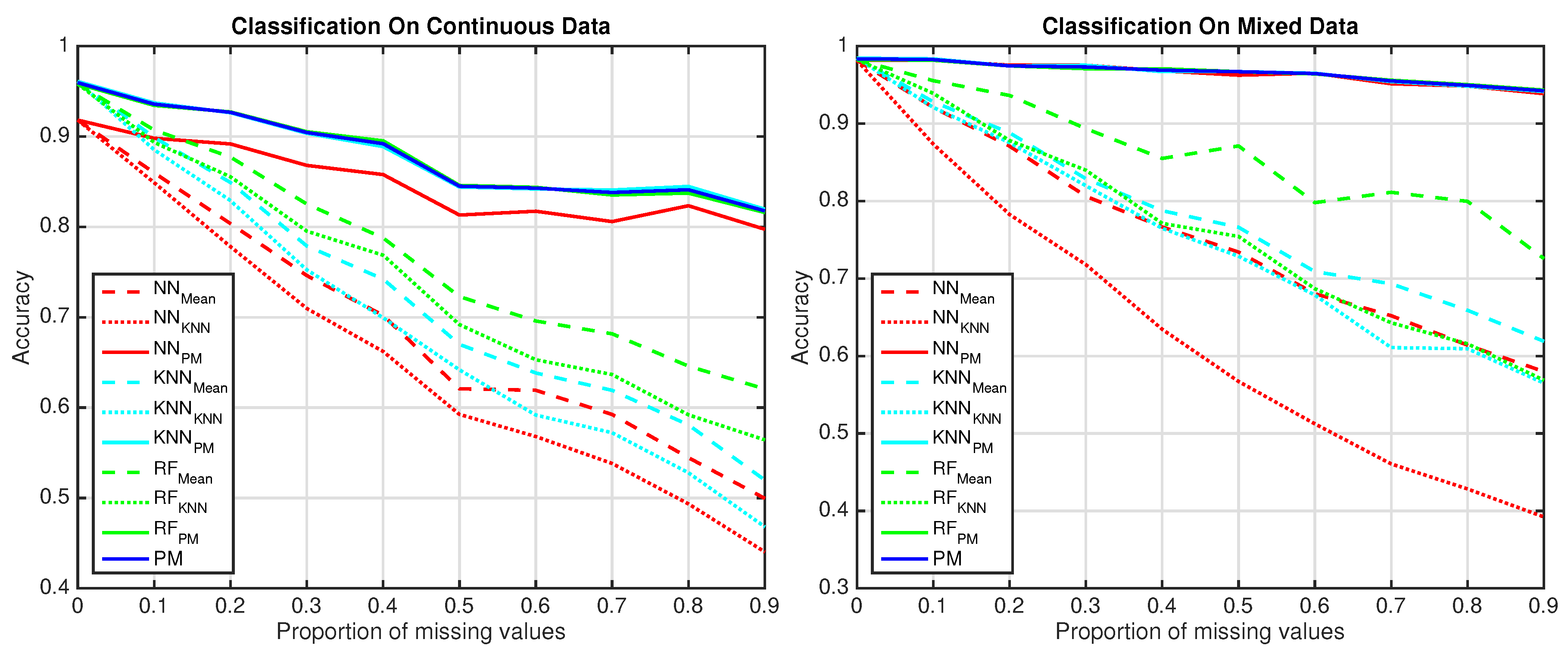
4.2. Classification Experiment

The classification experiment evaluates the ability of each algorithm to assign unlabeled data to one of the K classes trained by a set of labeled data. Since comparison algorithms do not handle datasets including missing values, a complete dataset is used to enable their training. During the prediction step, incomplete observations are completed thanks to the mean and KNN imputation methods and the posterior reconstructions defined in (6) and (7). For the classification experiment, results are shown in Figure 1. Without missing data, both algorithms cannot perfectly classify the 55 radar emitters for the 2 datasets. Indeed, both algorithms reach accuracies of $90\%$ for the continuous dataset and $98\%$ for the mixed dataset. These performance can be explained by the non total separability of continuous and categorical datasets since the 55 emitters share 42 combinations of categorical features and some intervals of continuous features. Nonetheless when mixed data are taken into consideration, the dataset becomes more separable leading to higher performance of both algorithms. When the proportion of missing values increases, the proposed model outperforms comparisons algorithms for each dataset. It achieves accuracies of $80\%$ and $95\%$ for $90\%$ of deleted continuous and mixed values whereas accuracies of comparison algorithms are lower than $65\%$ and $75\%$ with missing data imputation from standard methods. These higher performance of the proposed model reveal that the proposed method embeds a more efficient inference method than other imputation methods. That result is confirmed on Figure 1 when comparison algorithms are applied on data reconstructed by the proposed model. Indeed when the proposed inference is chosen, comparison algorithms share the same performance than the proposed model and manage to handle missing data even for $90\%$ of deleted values.

Then, effectiveness of the proposed model can be explained by the fact that missing data imputation methods can create outliers that deteriorate performance of classification algorithms whereas the inference on missing data and labels prediction are jointly estimated in the proposed model. Indeed, embedding the inference procedure into the model framework allows properties of the model, such as outliers handling, to counterbalance drawbacks of imputation methods such as outlier creation.

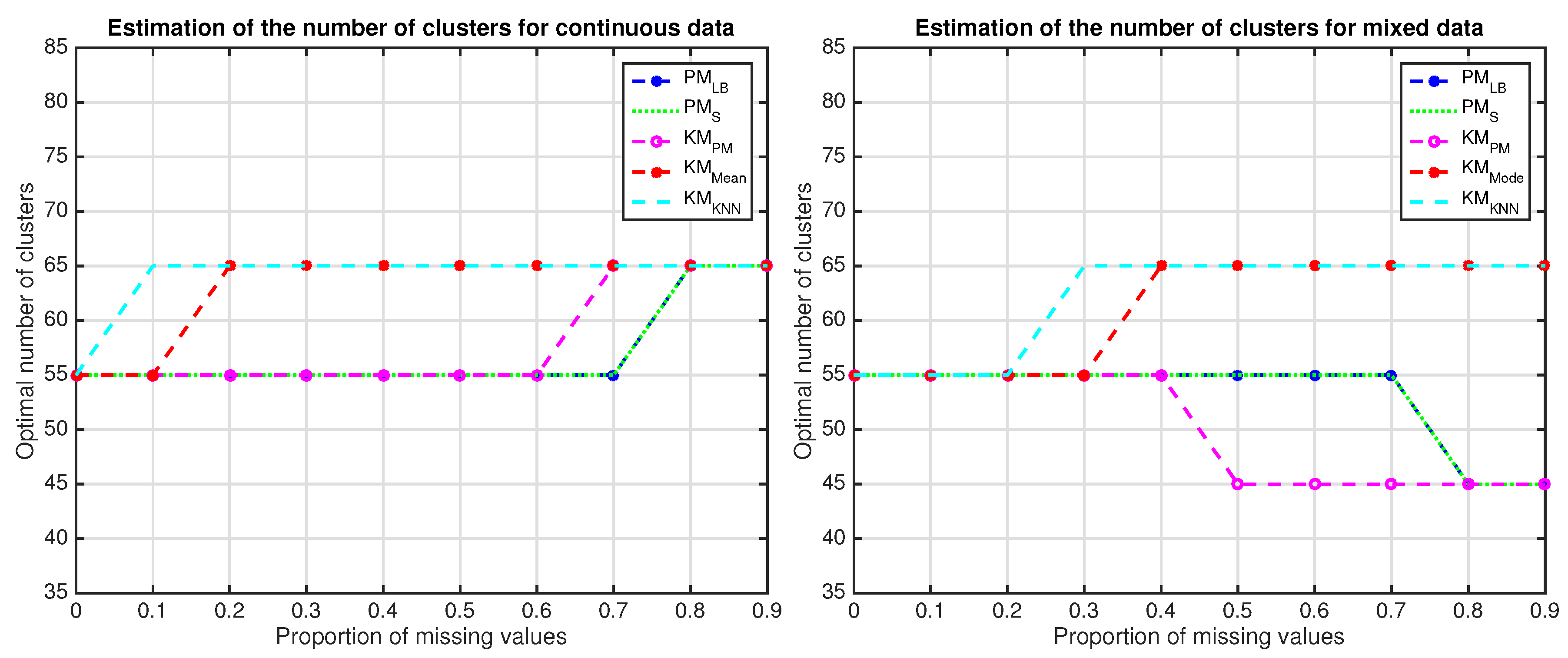
4.3. Clustering Experiment

The clustering experiment tests the ability of each algorithm to find the true number of clusters $\tilde{K}$ among $\{35,\dots ,85\}$. The lower bound (3) and the average Silhouette score [18] are criteria used to select the optimal number of clusters for the proposed model and the k-means algorithm. Results of the clustering experiment are visible on Figure 2 which presents numbers of clusters selected by the lower bound and average Silhouette scores for the proposed model and k-means algorithm according to different proportions of missing values and imputation methods. Without missing data, the correct number of clusters (K = 55) is selected by the two criteria for the k-means algorithm and the proposed model when continuous and mixed data are clustered. In presence of missing values, the average Silhouette score mainly selects $K=65$ when the k-means algorithm is run on the 2 datasets completed by standard imputation methods. When, the k-means algorithm performs clustering on the posterior reconstructions, the average Silhouette score correctly selects $K=55$ until $60\%$ of missing values for continuous data and $40\%$ of missing values for mixed data. Eventually when the proposed model does clustering, the two criteria select the correct number of clusters $K=55$ until $70\%$ of missing values for continuous and mixed data. These results show two main advantages of the proposed model. As previously, the proposed model provides a more robust inference on missing data since the average Silhouette score chooses more representative number of clusters when the k-means algorithm is run on the posterior reconstructions than on data completed by standard imputation methods. Furthermore, since the lower bound criterion also selects the correct number of clusters as the average Silhouette score, it can be used as a valid criterion for selecting the optimal number of clusters and does not require extra computational costs as the Silhouette score since it is computed during the model parameter estimation. Finally, the proposed approach provides a more robust inference on missing data and a criterion for selecting the optimal number of clusters without extra computations.

5. Conclusions

In this paper, a mixture model handling both continuous data and categorical data is developed. More precisely, an approach based on the conditional Gaussian mixture model is investigated by establishing conditional relations between continuous and categorical data. Benefiting from a dependence structure designed for mixed-type data, the proposed model shows its efficiency for inferring on missing data, performing classification and clustering tasks and selecting the correct number of clusters. Since the posterior distribution is intractable, model learning is processed through a variational Bayesian approximation where variational posterior distributions are proposed for continuous and categorical missing data. Experiments point out that the proposed approach can handle mixed-type data even in presence of missing values and can outperform standard algorithms in classification and clustering tasks. Indeed the main advantage of our approach is that it enables the counterbalance of imputation methods drawbacks by embedding the inference procedure into the model framework.

References

1. Bishop, C.M. Pattern Recognition and Machine Learning (Information Science and Statistics); Springer: Berlin/Heidelberg, Germany, 2006. [Google Scholar]
2. Hartigan, J.A.; Wong, M.A. Algorithm AS 136: A k-means clustering algorithm. J. R. Stat. Soc. Ser. C (Appl. Stat.) 1979, 28, 100–108. [Google Scholar] [CrossRef]
3. Ester, M.; Kriegel, H.P.; Sander, J.; Xu, X. A Density-Based Algorithm for Discovering Clusters in Large Spatial Databases with Noise; Kdd: Portland, OR, USA, 1996; Volume 96, pp. 226–231. [Google Scholar]
4. Breiman, L. Random forests. Mach. Learn. 2001, 45, 5–32. [Google Scholar] [CrossRef]
5. Sander, J.; Ester, M.; Kriegel, H.P.; Xu, X. Density-Based clustering in spatial databases: The algorithm GDBSCAN and its applications. Data Min. Knowl. Discov. 1998, 2, 169–194. [Google Scholar] [CrossRef]
6. Jain, A.K. Data clustering: 50 years beyond K-means. Pattern Recognit. Lett. 2010, 31, 651–666. [Google Scholar] [CrossRef]
7. Troyanskaya, O.; Cantor, M.; Sherlock, G.; Brown, P.; Hastie, T.; Tibshirani, R.; Botstein, D.; Altman, R.B. Missing value estimation methods for DNA microarrays. Bioinformatics 2001, 17, 520–525. [Google Scholar] [CrossRef] [PubMed]
8. Biernacki, C.; Celeux, G.; Govaert, G. Assessing a mixture model for clustering with the integrated completed likelihood. IEEE Trans. Pattern Anal. Mach. Intell. 2000, 22, 719–725. [Google Scholar] [CrossRef]
9. Lawrence, C.J.; Krzanowski, W.J. Mixture separation for mixed-mode data. Stat. Comput. 1996, 6, 85–92. [Google Scholar] [CrossRef]
10. Everitt, B. A finite mixture model for the clustering of mixed-mode data. Stat. Probab. Lett. 1988, 6, 305–309. [Google Scholar] [CrossRef]
11. Andrews, D.F.; Mallows, C.L. Scale Mixtures of Normal Distributions. J. R. Stat. Soc. Ser. B (Methodol.) 1974, 36, 99–102. [Google Scholar] [CrossRef]
12. Waterhouse, S.; MacKay, D.; Robinson, T. Bayesian methods for mixtures of experts. In Advances in Neural Information Processing Systems; MIT Press: Cambridge, MA, USA, 1996; pp. 351–357. [Google Scholar]
13. Schleher, D.C. Introduction to Electronic Warfare; Technical report; Eaton Corp., AIL Div.: Deer Park, NY, USA, 1986. [Google Scholar]
14. Richards, M.A. Fundamentals of Radar Signal Processing; McGraw-Hill Education: New York, NY, USA, 2005. [Google Scholar]
15. Akaike, H. Information theory and an extension of the maximum likelihood principle. In Selected Papers of Hirotugu Akaike; Springer: New York, NY, USA, 1998; pp. 199–213. [Google Scholar]
16. Schwarz, G. Estimating the dimension of a model. Ann. Stat. 1978, 6, 461–464. [Google Scholar] [CrossRef]
17. García-Laencina, P.J.; Sancho-Gómez, J.L.; Figueiras-Vidal, A.R. Pattern classification with missing data: A review. Neural Comput. Appl. 2010, 19, 263–282. [Google Scholar] [CrossRef]
18. Kaufman, L.; Rousseeuw, P.J. Finding Groups in Data: An Introduction to Cluster Analysis; John Wiley & Sons: Hoboken, NJ, USA, 2009; Volume 344. [Google Scholar]
Figure 1. Classification performance are presented for the proposed model (PM) in blue, the NN in red, the RnF in green and the KNN in cyan. For each figure, solid lines represent accuracies with a posteriori reconstructed missing data, doted dashed lines stand for accuracies with mean/mode imputation whereas dashed lines show accuracies with KNN imputation for the comparison algorithms.
Proceedings 33 00023 g001
Figure 2. Estimation of the number of clusters using the lower bound (LB) and the silhouette score (S) for the proposed model and only the silhouette score (S) for the k-means algorithm.
Proceedings 33 00023 g002