On the Diagnosis of Aortic Dissection with Impedance Cardiography: A Bayesian Feasibility Study Framework with Multi-Fidelity Simulation Data ^†

Abstract

Aortic dissection is a cardiovascular disease with a disconcertingly high mortality. When it comes to diagnosis, medical imaging techniques such as Computed Tomography, Magnetic Resonance Tomography or Ultrasound certainly do the job, but also have their shortcomings. Impedance cardiography is a standard method to monitor a patients heart function and circulatory system by injecting electric currents and measuring voltage drops between electrode pairs attached to the human body. If such measurements distinguished healthy from dissected aortas, one could improve clinical procedures. Experiments are quite difficult, and thus we investigate the feasibility with finite element simulations beforehand. In these simulations, we find uncertain input parameters, e.g., the electrical conductivity of blood. Inference on the state of the aorta from impedance measurements defines an inverse problem in which forward uncertainty propagation through the simulation with vanilla Monte Carlo demands a prohibitively large computational effort. To overcome this limitation, we combine two simulations: one simulation with a high fidelity and another simulation with a low fidelity, and low and high computational costs accordingly. We use the inexpensive low-fidelity simulation to learn about the expensive high-fidelity simulation. It all boils down to a regression problem—and reduces total computational cost after all.

1. Introduction

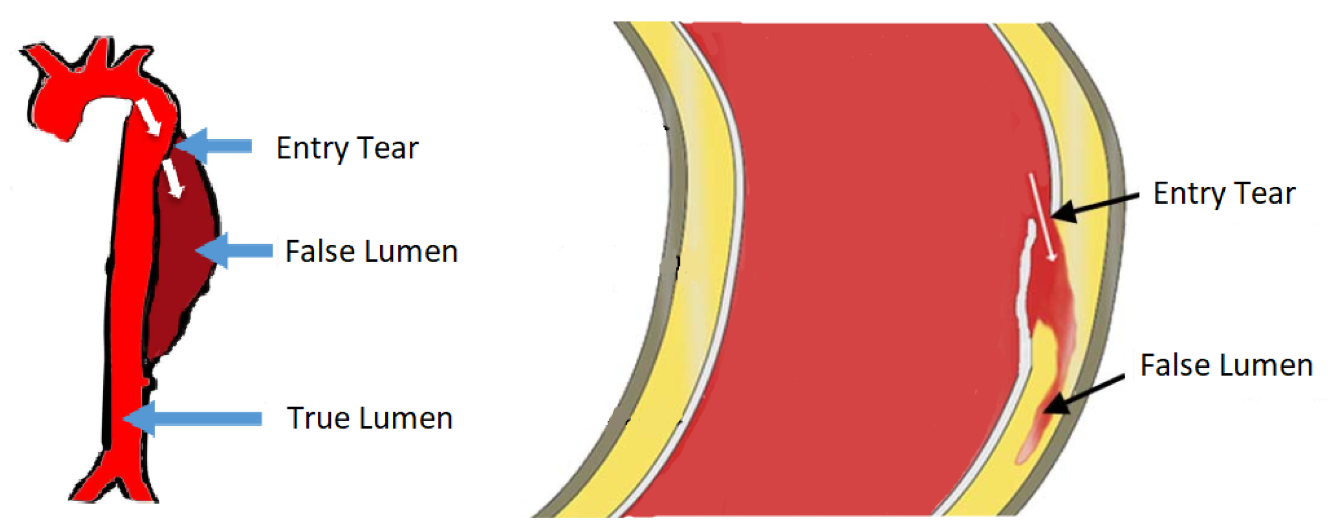
The largest blood vessel in the human body is the aorta. The wall of the aorta is made of aortic tissue, a layered composition of muscle cells, collagen, elastin fibres, etc. In Aortic Dissection (AD), a tear in the innermost layer of the aortic wall permits blood to flow in between the layers, effectively forcing apart the layers and deforming the geometry of the aorta. Obviously, AD affects blood circulation unfavourably ([1] p. 459). This pathology is illustrated in Figure 1.

The condition AD is often acute and requires immediate treatment, but diagnosis is difficult. Physicians use a variety of imaging techniques to diagnose AD, among which are Magnetic Resonance Tomography (MRT), Computed Tomography (CT) and Echocardiography, the latter of which is based on an ultrasound device [3]. Ultrasound devices are comparably cheap, fast and easy to handle. But if wave propagation is obfuscated by, e.g., the rib cage, the technique is not applicable. CT and MRT do not have this limitation due to full radiation penetration of the body, but show a number of drawbacks: long measurement times, radiation exposure, high costs, require specialized personnel (radiologists) and most importantly, MRT/CT is not available on a whim. A fast response, and a fast diagnosis, hence, is key to the treatment of AD patients. 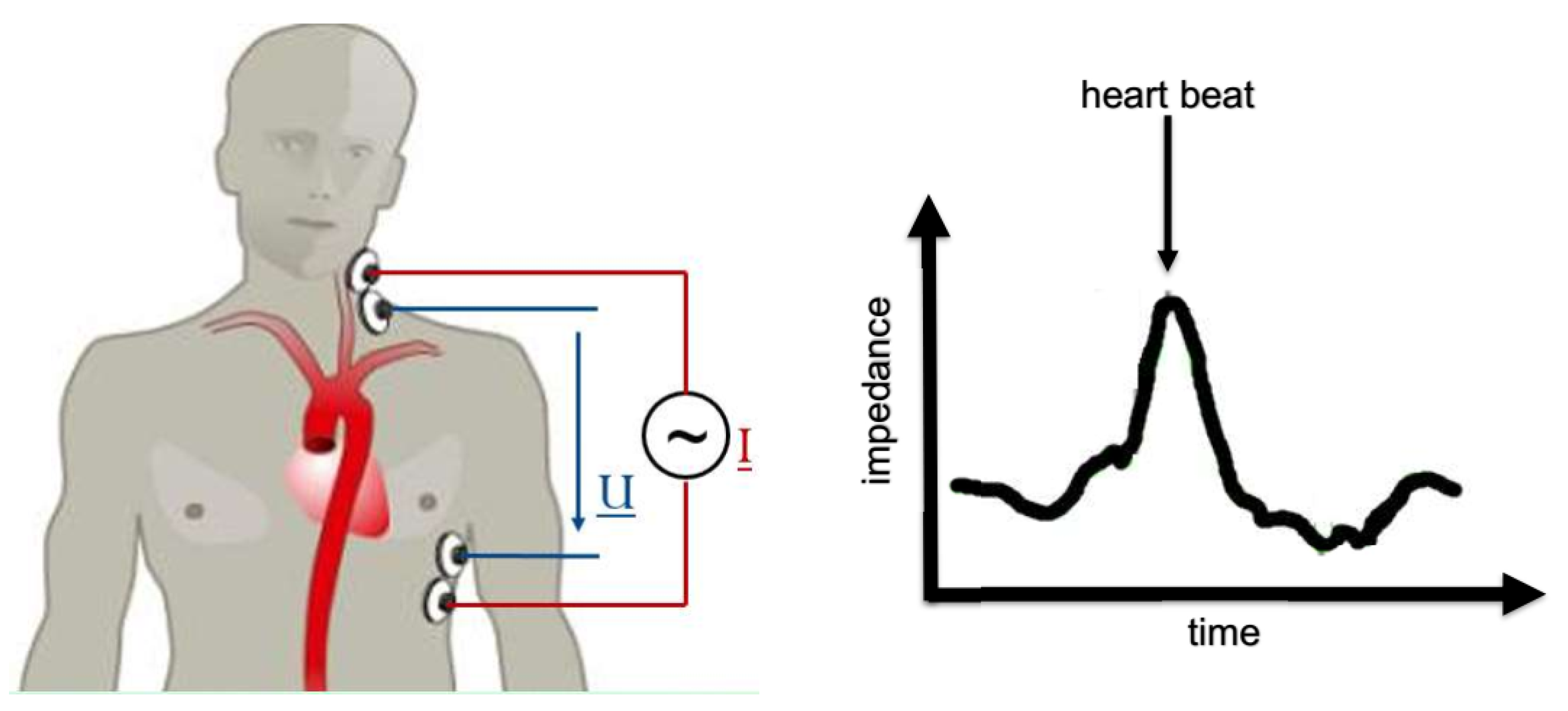In this work, we analyse the proposal of [4] to use impedance cardiography (ICG) [5] for AD diagnosis. In ICG, one places a pair of electrodes on the thorax (upper body), injects a defined low-amplitude, alternating electric current into the body and measures the voltage drop. The generic experimental setup is illustrated in Figure 2. The specific al resistance (impedance) of blood is much lower than that of muscle, fat or bone [6]. Electric current seeks the path of least resistance, and thus the current propagates through the aorta rather than through, e.g., the spine. If blood is redistributed within the body due to AD, the path of least resistance is expected to change, and so the overall resistance of the body. ICG is bad to distinguish between different types of blood redistribution, e.g., AD or lung edema [7]. Still, ICG yields yet another clue in a physician’s diagnostic procedure. ICG is fast, cheap, available on a whim and does not require specialized personnel. A new medical detection device based on ICG would thus close a gap left open by existing procedures.

To develop such a device, it is necessary to perform experiments which are extraordinarily difficult, both technically as well as ethically. One would need ICG measurements as well as high quality tomography data stemming from the same person, before and after AD happened. That kind of data is not available, and we resort to Finite Element (FE) simulations [8] instead. In these simulations, we find a number of input parameters which are well-defined, but usually neither known precisely nor accessible in the clinical setting. For example, a patient’s blood conductivity varies from day to day. The input parameters are thus afflicted with uncertainty, and this uncertainty propagates through the simulation to the output, which here is the measured impedance. If we wanted a meaningful statement on the condition of the aorta, we therefore need to quantify the uncertainty in the measurement. It is an inverse problem, which involves the forward Uncertainty Quantification (UQ) first. UQ has become a term on its own in the engineering community. A rather chunky, but quite comprehensive collection of reviews on the various aspects of UQ can be found in Reference [9]. A Bayesian perspective is discussed in [10,11,12].

UQ usually requires quite some computational effort, depending on the number of uncertain parameters and the computational cost of a single simulation itself. If this computational effort is prohibitively large, one may use a surrogate model. The two most widely used surrogate models are Polynomial Chaos Expansion (PCE) [13,14,15,16] and Gaussian Process Regression (GPR) [17,18]. PCE is particularly widely spread within then engineering community, while GPR has had its renaissance recently within the machine learning community [19,20].

This work is inspired by the article of Kennedy and O’Hagan in 2000 [21]. They performed UQ by making use of a computer simulation with different levels of ‘sophistication’ or ‘fidelity’. In other words, a cheap simplified simulation serves as a surrogate. Koutsourelakis follows this idea later on [22]. While UQ in general has arrived fully in the Biomedical Engineering community [23], the Bayesian approach has not. Biehler et al. [24] were, to the best knowledge of the authors, the first to apply a Bayesian Multi-Fidelity Scheme in the context of computational Bio-mechanics .

In Section 2 we build a physical model of an impedance cardiography measurement applied to the described physiological system. In Section 3, we develop a Bayesian Multi-Fidelity scheme, which is then used for Uncertainty Quantification of the physical model. The results, i.e., the uncertainty bands of the ICG signal, are presented and discussed in Section 4. We draw our conclusions and suggest possible future improvements in Section 5.

2. The Physical Model

We start from the Maxwell’s equations and recognize that one cardiac cycle, i.e., the time span between two heart beats, is on the order of one second, and the frequency of the injected current is on the order of a hundred kilo-Hertz. Thus we can assume the electric field to be quasi-static [4], and the Maxwell equations boil down to Laplace’s equation (in complex notation),

$$\nabla \left((\sigma +i\omega \epsilon )\nabla V\right)=0,$$

(1)

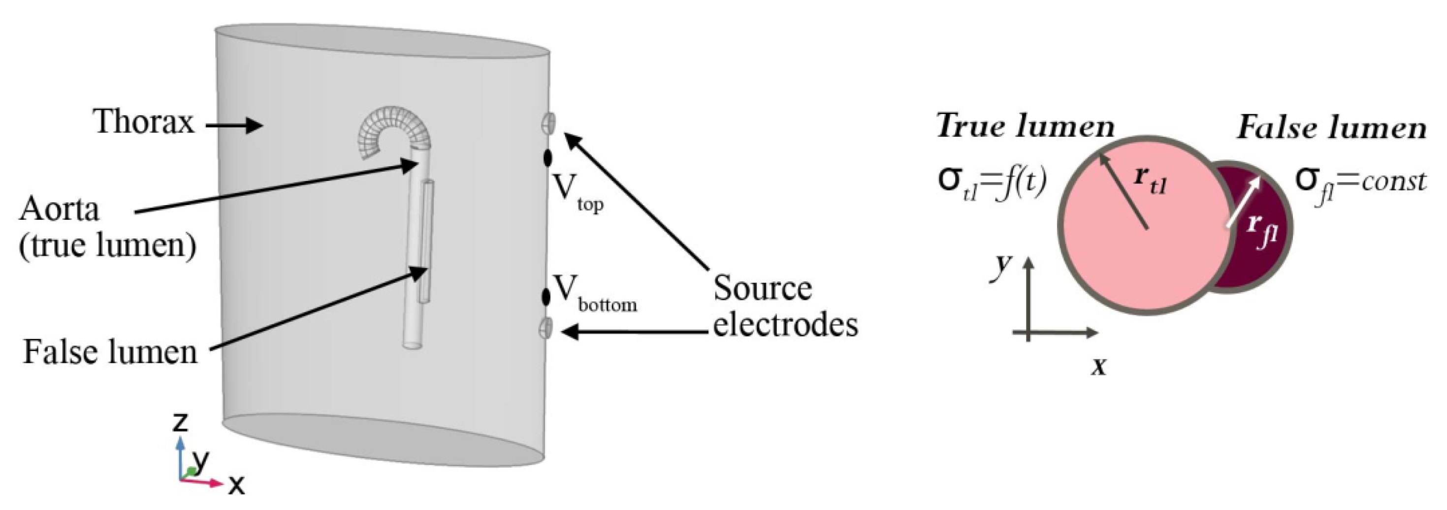
with electric potential V, electrical conductivity $\sigma$, angular frequency $\omega$, permittivity $\epsilon$ and imaginary unit i. Equation (1) is then to be solved on the geometry as depicted in Figure 3 and described as follows. The thorax (upper body) is modelled by an elliptic cylinder with a spatially homogeneous conductivity and permittivity. The aorta is an up-side-down umbrella stick. We consider the whole organ to be filled with blood and neglect the vessel walls. In clinical parlance, the blood-filled cavity caused by the aortic dissection is called “false lumen”, while the anatomically correct cavity is called “true lumen”. The true lumen is modelled as a circular cylinder, and the false lumen is a holed out circular cylinder attached to the true lumen. The dynamics are modelled via a time-dependent true and false lumen radius, which arises from pressure waves in a pulsatile flow. Further, the blood conductivity depends on the blood flow velocity, and is thus time-dependent in the true lumen, but constant in the false lumen due to a negligible flow velocity [4,25]. The boundary conditions are specified by the body surface and two source electrodes. The two source electrodes are modelled by two patches (top and bottom) on the left-hand side of the patient. For the top patch, the injection current is held constant at 4 mA and a frequency of 100 kHz via a constant surface integral of the current density. The bottom patch is defined as ground, i.e., a constant voltage ${\mathrm{V}}_{\mathrm{bottom}}=0$ V. Considering the relatively low conductivity of air, we assume the rest of the body surface to be perfectly insulating. Equation (1) is then discretized in space and solved with the Finite Elements method [8]. The quality and fidelity of the space discretization, colloquially termed as “the mesh”, is crucial to the quality of the solution, but also to the amount of computational effort. We use a rather coarse mesh of low fidelity, and a rather detailed mesh of high fidelity, with two examples illustrated in Figure 4.

We distinguish observable and unobservable (uncertain) parameters (also termed hidden or latent variables). An obvious observable parameter is time t. From the plethora of unobservable parameters, we choose the false lumen radius, $r_{fl}$, and perform a number of simulations with sensible values within the physiological and physical range, i.e., 5.0–25.0 mm with a step size of $1.0$ mm. The physical lower boundary would be 0 mm, yet below 5 mm meshing problems occur in the LoFi model, i.e., badly shaped elements become frequent, geometry is approximated badly and thus space discretization fails. This is not surprising, since the LoFi model’s size of finite elements is on the order of $5.0$ mm, and therefore cannot exhibit features of more detail. For any simulation, the voltage drop between any two points can now be measured. In the clinical setting, there would be a number of probe electrodes attached to the patient’s chest, back, neck and/or limbs, and voltage drops measured between the many pairs of probe electrodes. Here, we limit ourselves to just one pair of probe electrodes, with one probe electrode right beneath the upper injection electrode, and one probe electrode right above the lower injection electrode. The positions of the probe electrodes, relative to the injection electrodes, are indicated in Figure 3 by V_top and V_bottom.

We used the Comsol Multiphysics software to perform the modelling [26].

3. Bayesian Multi-Fidelity Scheme

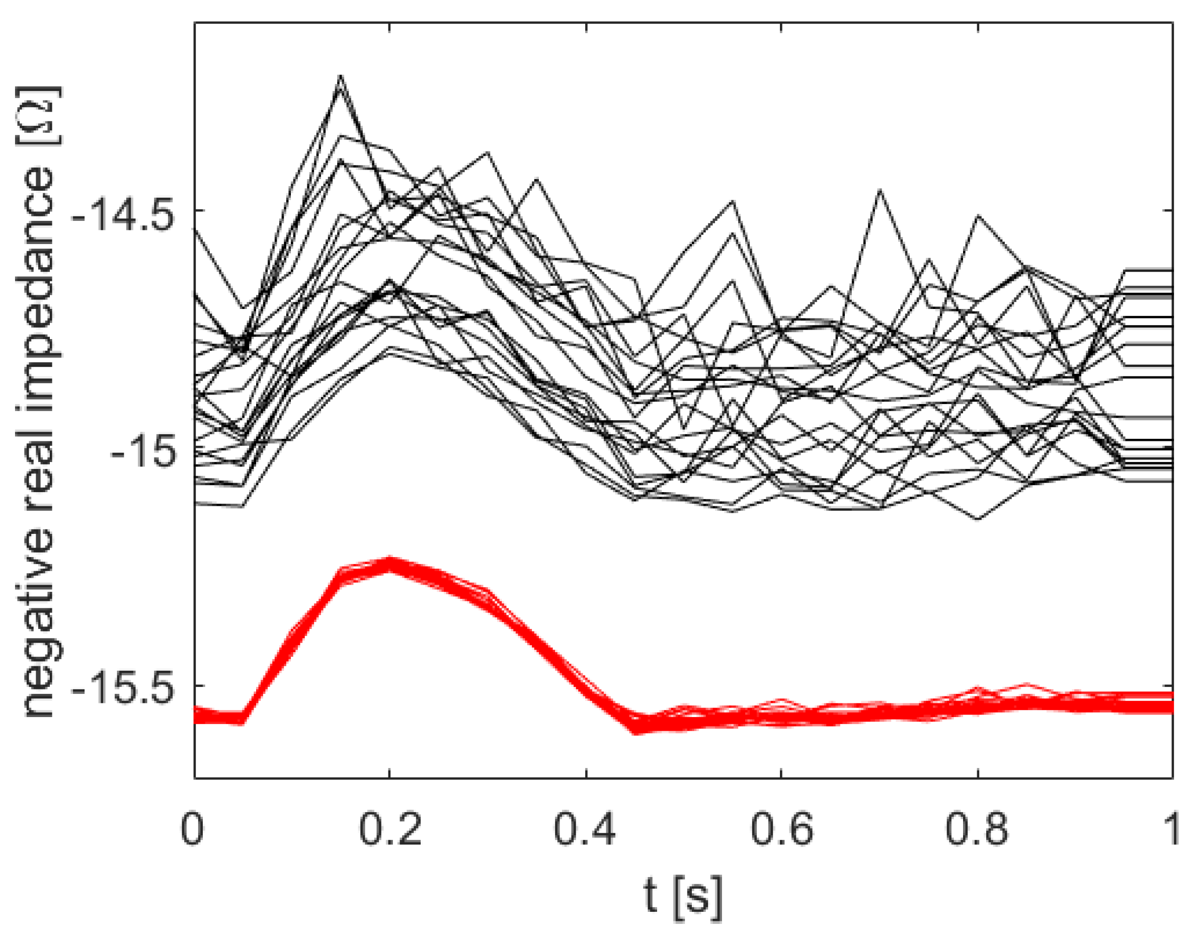
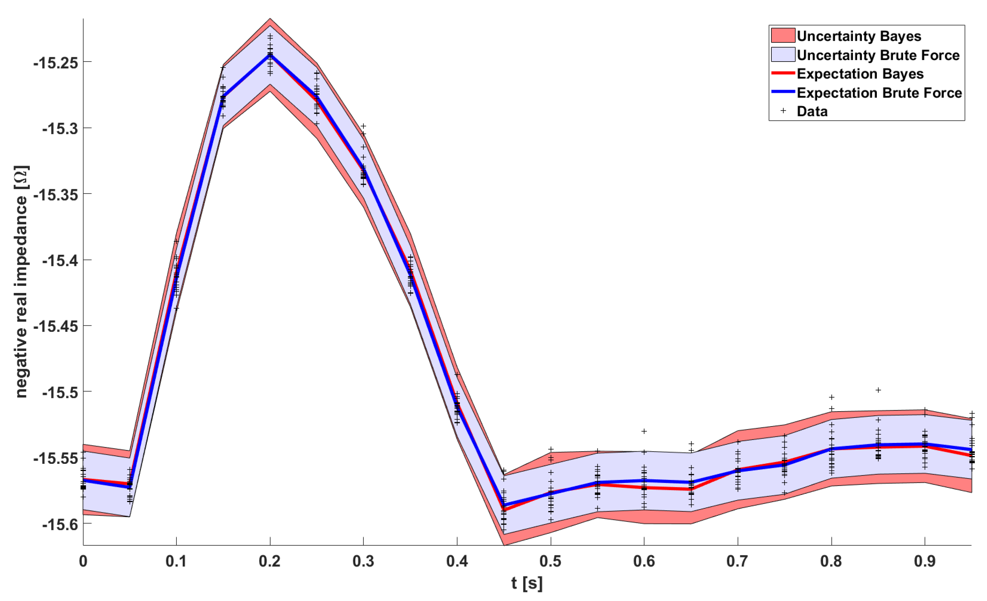
Having computed all the HiFi impedance times series (red) in Figure 5, the uncertainty quantification is pretty much done already. The uncertainty bands of the Brute Force HiFi data in Figure 6 (blue) are inferred from a Gaussian Process model with a squared exponential kernel. In the following paragraphs we will instead use the LoFi impedance time series (black) and only a few of the data points of the HiFi impedance time series (red). In other words; in order to compute the uncertainty bands, instead of doing all the HiFi simulations, we rather do all the LoFi simulations and only a few HiFi simulations.

We distinguish the observable physical parameter time, t, from unobservable (uncertain) physical parameters $\xi$. We consider two disjoint data sets, $D_1$ and $D_2$. $D_1$ is a large set of input parameters, ${\overrightarrow{\xi }}_1={\left\{{\xi }_1^{\left(i\right)}\right\}}_{i=1}^{N_{\xi ,1}}$, ${\overrightarrow{t}}_1={\left\{t_1^{\left(k\right)}\right\}}_{k=1}^{N_{t,1}}$, and corresponding (noisy) outputs of the LoFi model, ${\overrightarrow{V}}_{L,1}={\left\{V_{L,1}^{(i,k)}\right\}}_{i,k=1}^{N_{\xi ,1},N_{t,1}}$, where each individual output $V_{L,1}^{(i,k)}$ is the voltage drop with parameter ${\xi }_1^{\left(i\right)}$ at time instance $t_1^{\left(k\right)}$. ${\overrightarrow{t}}_1$ covers the time series of one whole cardiac cycle. This means $D_1=\{{\overrightarrow{t}}_1,{\overrightarrow{\xi }}_1,{\overrightarrow{V}}_{L,1}\}={\left\{(t_1^{\left(k\right)},{\xi }_1^{\left(i\right)},V_{L,1}^{(i,k)})\right\}}_{i,k=1}^{N_{\xi ,1},N_{t,1}}$. In principle, the solver is deterministic, yet the solution depends on the mesh. Since the false lumen radius is treated as a random variable, the geometry is random as well, and each mesh a specific realization of it. We then choose a small subset of the outputs of $D_1$ with size $N_{\xi ,2}$, and $N_{t,2}$ respectively, for which we additionally compute the (noisy) HiFi solution. This subset is chosen such that the support of ${\overrightarrow{V}}_{L,1}$ is appropriately covered. Given input parameters ${\overrightarrow{\xi }}_2={\left\{{\xi }_2^{\left(i\right)}\right\}}_{i=1}^{N_{\xi ,2}}$, ${\overrightarrow{t}}_2={\left\{t_2^{\left(k\right)}\right\}}_{k=1}^{N_{t,2}}$, the corresponding output of the HiFi model is ${\overrightarrow{V}}_{H,2}={\left\{V_{H,2}^{(j,m)}\right\}}_{j,m=1}^{N_{\xi ,2},N_{t,2}}$. We gather these tuples of LoFi-output and corresponding HiFi-output in data set $D_2=\{{\overrightarrow{t}}_2,{\overrightarrow{\xi }}_2,{\overrightarrow{V}}_{L,2},{\overrightarrow{V}}_{H,2}\}={\left\{(t_2^{\left(m\right)},{\xi }_2^{\left(j\right)},V_{L,2}^{(j,m)},V_{H,2}^{(j,m)})\right\}}_{j,m=1}^{N_{\xi ,2},N_{t,2}}$. In other words, $D_2$ shall be a small subset of $D_1$ which “in hindsight” is augmented with the corresponding HiFi data.

We acknowledge that time t is observable in our experiment, but the latent variables $\xi$ are not. Let $V_H^{*}$ and $V_L^{*}$ be the true values of high fidelity and low fidelity model respectively, corresponding to given input parameters (latent variables) $\xi$ and a time instance t. Note the distinction of the true values $V_H^{*}$ and $V_L^{*}$ from the noisy observations in $D_1$ and $D_2$. Let $\mathcal{C}$ be the conditional complex. We want to compute the uncertainty bands of the ICG signal in Figure 5, meaning the posterior pdf of $V_H^{*}$ given t, and introduce $V_L^{*}$ via marginalisation

$$p(V_H^{*}\mid t,D_1,D_2,\mathcal{C})=\int p(V_H^{*}\mid V_L^{*},t,\cancel{D_1},D_2,\mathcal{C})p(V_L^{*}\mid t,D_1,\cancel{D_2},\mathcal{C})d{V}_L^{*},$$

(2)

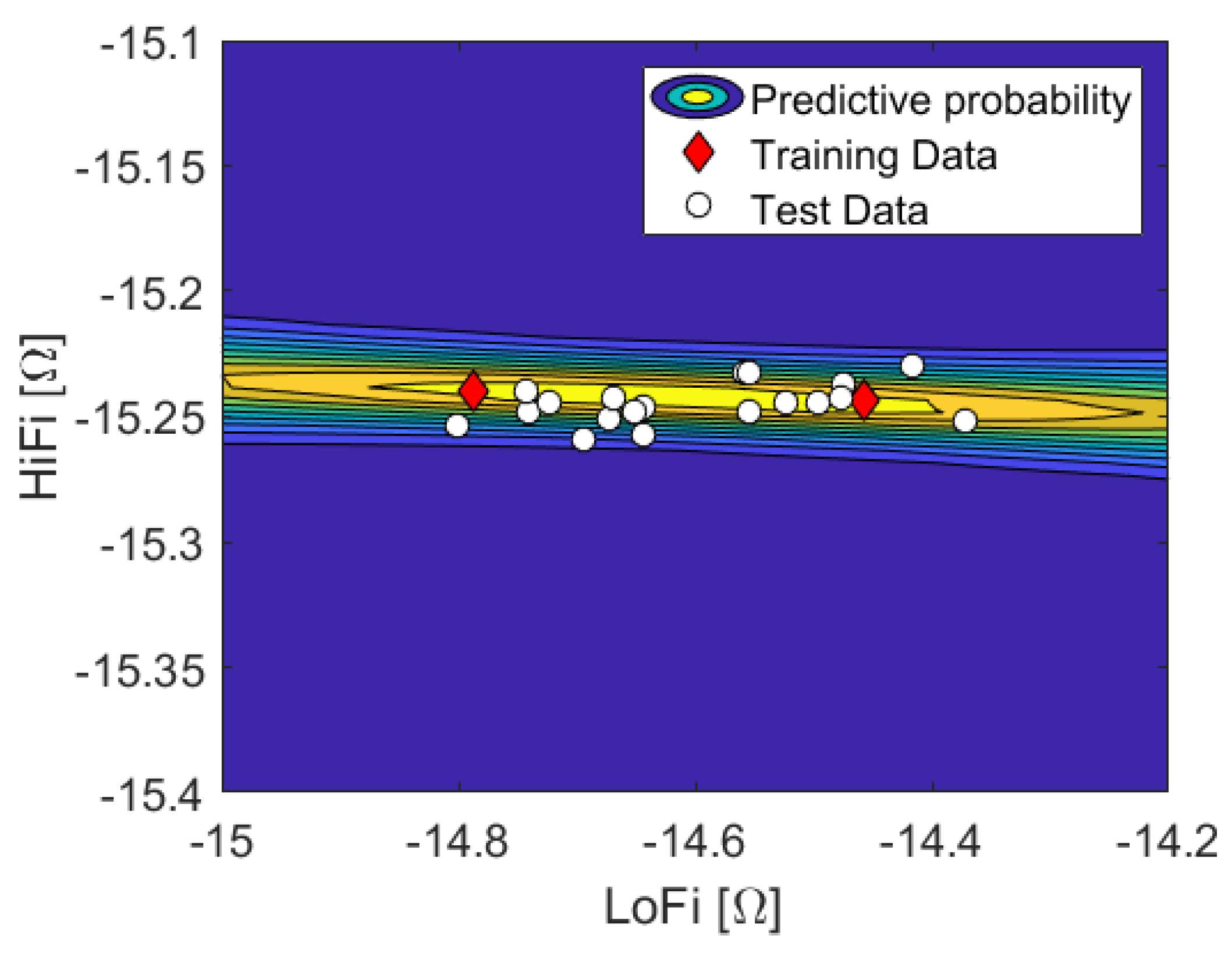
where we constructed the data sets such that we can partially cross them out here. For the sake of easier notation, we will omit the conditional complex $\mathcal{C}$ from here on. Let us first discuss the first term in the integral. It implies a one-dimensional regression problem $V_L^{*}\mapsto V_H^{*}$. This is convenient since the original problem, $\xi \mapsto V_H^{*}$ , is usually multi-dimensional, and will come in handy once we scale up the number of uncertain parameters. We need to choose a regression function f, acknowledge noise induced by the discretization error with $\sigma$, and marginalize f’s hyperparameters $\theta$, i.e.,

$$p(V_H^{*}\mid V_L^{*},t,D_2,f,\sigma )=\int p(V_H^{*}\mid V_L^{*},t,\cancel{D_2},f,\sigma ,\theta )p(\theta \mid \cancel{V_L^{*}},t,D_2,f,\sigma )d\theta$$

(3)

Note that f is actually included in the conditional complex $\mathcal{C}$, but explicitly written out here. In Equation (3), we find a belated, formal justification for replacing the original regression problem $\xi \mapsto V_H^{*}$. In the conditional pdf in Equation (3), $\mathcal{C}$ implies that the knowledge of f, $\theta$, and $V_L^{*}$ already determines $V_H^{*}$ apart from noise $\sigma$, and thus $D_2$ is superfluous.

By looking at the data, we recognize that a linear regression function $f_{}^{}$ will capture the salient features, and is hence sufficient for all time instances. Thus the prior reads

$$p(\theta \mid f)=p(a,b\mid f,a_0,b_0)=a_0{(1+a)}^{-3/2}\Theta (\mid b\mid \le b_0),$$

(4)

with inclination a, constant offset b and $\Theta$ being the Heaviside function. We find no apparent outliers in the data, and the likelihood shall be Gaussian with constant noise level, which was estimated from the data to $\sigma =0.01$.

The second term in Equation (2) is approximated by weighted samples ($D_1$), and the integral boils down to a discreet sum over these.

4. Results & Discussion

An example of the intermediate result of Equation (3) is shown in Figure 7. We see the predictive probability of the HiFi impedance given the LoFi impedance for the time instance at peak systole ($t=200$ ms). Naturally, linear regression requires at least two training data points, which was deemed good enough in this experiment. In Figure 6, one can see the final result in comparison to the reference solution, i.e., with all the HiFi simulations. Expectations as well as uncertainties ($2\sigma$) match the reference solution quite well in the time range of 0–500 ms (systolic part), while the uncertainties in the time range 500–1000 ms (diastolic part) are a bit larger. This is reasonable, since the discretisation error in this regime is notably higher, which is obvious from the data, Figure 5. Since changes to the impedance due to aortic dissection are particularly expected to arise in the systolic part, we find the result satisfying nevertheless. The computational effort is documented in

Table 1. Comparison of computational resources. Each experiment was performed on 20 cores in parallel (with trivial parallelization) on Xeon E5-2640 with 8GB RAM/CPU. Degrees of freedom vary from time instance to time instance since the aortic radius is a function of time. In Figure 6, we compare the Brute Force HiFi results (blue) with the Bayesian HiFi results (red). The LoFi results are a mere means to compute the Bayesian HiFi results and thus not shown, yet their computational effort is documented since needed to quantify the reduction of the computational effort.

Model	Degrees of Freedom	Samples	CPU Time [s]	Wall Clock Time [s]
LoFi	9000–15,000	25	39,500	1975
Brute Force HiFi	100,000–550,000	25	192,480	9624
Bayesian HiFi		25 LoFi, 2 HiFi	54955	2748

. The Bayesian Multi-fidelity scheme reduces the computational effort roughly by a factor of 3.5. This might seem disappointing at first, but is actually quite close to the theoretical limit of a factor of 4, which is determined by the ratio of computational effort of one LoFi simulation over one HiFi simulation, and specific for any experiment thus. Specifically, the HiFi computational effort is defined by the user’s desired fidelity, e.g., mesh convergence, while the LoFi computational effort is determined by the HiFi model’s cheapest simplification which still shows statistical correlation with the HiFi model.

5. Conclusions & Outlook

We have set up a framework to systematically study the uncertainties of theoretical impedance cardiography signals associated with aortic dissection. Since the computational effort is about to skyrocket soon, we employed a Bayesian multi-fidelity scheme rather than using brute force. We did first experiments as a proof of principle, and computed the uncertainty bands of the simulation given an unknown false lumen radius. We achieved a solution quantitatively comparable to the reference solution, while reducing computational effort by roughly a factor of 3.5, which is close to the theoretical limit of 4. With increasing computational effort per simulation, we expect the reduction factor to increase.

The physical model will be improved by adding organs (e.g., lungs, heart) to the model one by one, and dispersion effects investigated by varying the injection current frequency (i.e., the boundary conditions). In terms of data analysis, the next step is to make further use of the pronounced structure of the signal, and sparsify simulation runs of the HiFi model in the time domain. This could be done by, e.g., interpreting each time series as a sample drawn from a Gaussian Process. i.e., we impose a GP prior onto the signal. Ultimately, we want to answer the inverse problem, “Is the aorta healthy or dissected?”, and thus need to compute the evidences. We strongly believe that this question can only be answered unambiguously by considering the signals of multiple electrodes at different positions on the human body at once.

References

1. Humphrey, J.D. Cardiovascular Solid Mechanics; Springer: New York, NY, USA, 2002; p. 459. [Google Scholar] [CrossRef]
2. Heuser, J. Distributed under a CC-BY-SA-3.0 License; Tech. Rep.; Wikimedia Commons: Omaha, NE, USA, 2016. [Google Scholar]
3. Khan, I.A.; Nair, C.K. Clinical, diagnostic, and management perspectives of aortic dissection. Chest 2002, 122, 311–328. [Google Scholar] [CrossRef] [PubMed]
4. Reinbacher-Köstinger, A.; Badeli, V.; Biro, O.; Magele, C. Numerical Simulation of Conductivity Changes in the Human Thorax Caused by Aortic Dissection. IEEE Trans. Magn. 2019, 55, 1–4. [Google Scholar] [CrossRef]
5. Miller, J.C.; Horvath, S.M. Impedance Cardiography. Psychophysiology 1978, 15, 80–91. [Google Scholar] [CrossRef] [PubMed]
6. Gabriel, C.; Gabriel, S.; Corthout, E.C. The dielectric properties of biological tissues: I. Literature survey. Phys. Med. Biol. 1996, 41, 2231–2249. [Google Scholar] [CrossRef] [PubMed]
7. De Sitter, A.; Verdaasdonk, R.M.; Faes, T.J. Do mathematical model studies settle the controversy on the origin of cardiac synchronous trans-thoracic electrical impedance variations? A systematic review. Physiol. Meas. 2016, 37, R88–R108. [Google Scholar] [CrossRef] [PubMed]
8. Zienkiewicz, O.C.; Taylor, R.L.; Zhu, J.Z. The Finite Element Method: Its Basis and Fundamentals; Elsevier: London, UK, 1967. [Google Scholar]
9. Ghanem, R.G.; Owhadi, H.; Higdon, D. Handbook of Uncertainty Quantification; Springer: New York, NY, USA, 2017. [Google Scholar] [CrossRef]
10. Haylock, R. Bayesian Inference about Outputs of Computationally Expensive Algorithms with Uncertainty on the Inputs. Ph.D. Thesis, Universtity of Nottingham, Nottingham, UK, 1997. Available online: http://eprints.nottingham.ac.uk/13193/1/338522.pdf (accessed on 22 November 2019).
11. O’Hagan, A.; Kennedy, M.C.; Oakley, J.E. Uncertainty analysis and other inference tools for complex computer codes. In Bayesian Staistics 6; Oxford Science Publications: Oxford, UK, 1999; pp. 503–524. [Google Scholar]
12. O’Hagan, A. Bayesian analysis of computer code outputs: A tutorial. Reliab. Eng. Syst. Saf. 2006, 91, 1290–1300. [Google Scholar] [CrossRef]
13. Wiener, N. The Homogeneous Chaos. Am. J. Math. 1938, 60, 897–936. [Google Scholar] [CrossRef]
14. Ghanem, R.G.; Spanos, P.D. Stochastic Finite Elements: A Spectral Approach; Springer: New York, NY, USA, 1991. [Google Scholar] [CrossRef]
15. Xiu, D.; Karniadakis, G.E. The Wiener-Askey polynomial chaos for stochastic differential equations. SIAM J. Sci. Comput. 2005, 27, 1118–1139. [Google Scholar] [CrossRef]
16. O’Hagan, A. Polynomial Chaos: A Tutorial and Critique from a Statistician’s Perspective. Available online: http://tonyohagan.co.uk/academic/pdf/Polynomial-chaos.pdf (accessed on 25 June 2019).
17. O’Hagan, A. Curve Fitting and Optimal Design for Prediction. J. R. Stat. Soc. Ser. B (Methodol.) 1978, 40, 1–42. [Google Scholar] [CrossRef]
18. Rasmussen, C.E.; Williams, C.K. Gaussian Processes for Machine Learning; The MIT Press: Cambridge, MA, USA, 2006. [Google Scholar] [CrossRef]
19. Bishop, C. Neural Networks for Pattern Recognition; Oxford University Press: Oxford, UK, 1996. [Google Scholar]
20. MacKay, D.J. Information Theory, Inference, and Learning Algorithms; Cambridge University Press: Cambridge, UK, 2003. [Google Scholar] [CrossRef]
21. Kennedy, M.C.; O’Hagan, A. Predicting the output from a complex computer code when fast approximations are available. Biometrika 2000, 87, 1–13. [Google Scholar] [CrossRef]
22. Koutsourelakis, P.S. Accurate Uncertainty Quantification using inaccurate Computational Models. SIAM J. Sci. Comput. 2009, 31, 3274–3300. [Google Scholar] [CrossRef]
23. Eck, V.G.; Donders, W.P.; Sturdy, J.; Feinberg, J.; Delhaas, T.; Hellevik, L.R.; Huberts, W. A guide to uncertainty quantification and sensitivity analysis for cardiovascular applications. Int. J. Numer. Methods Biomed. Eng. 2016, 32, e02755. [Google Scholar] [CrossRef] [PubMed]
24. Biehler, J.; Gee, M.W.; Wall, W.A. Towards efficient uncertainty quantification in complex and large-scale biomechanical problems based on a Bayesian multi-fidelity scheme. Biomech. Model. Mechanobiol. 2015, 14, 489–513. [Google Scholar] [CrossRef] [PubMed]
25. Alastruey, J.; Xiao, N.; Fok, H.; Schaeffter, T.; Figueroa, C.A. On the impact of modelling assumptions in multi-scale, subject-specific models of aortic haemodynamics. J. R. Soc. Interface 2016, 13. [Google Scholar] [CrossRef] [PubMed]
26. Comsol, A.B.; Stockholm, S. Comsol Multiphysics Version 5.4. Available online: http://www.comsol.com (accessed on 4 June 2019).
Figure 1. Illustration of a dissected aorta. Left: The whole organ. Right: Close-up to the entry tear [2]. Blood pushes from the anatomically correct cavity (medical parlance: true lumen) through a tear into the aortic wall. The tear grows and builds another cavity (medical parlance: false lumen), affecting blood circulation unfavourably.
Proceedings 33 00024 g001
Figure 2. Left: Experimental setup of ICG. Right: Generic ICG signal.
Proceedings 33 00024 g002
Figure 3. Left: CAD Model of Thorax with dissected Aorta. Right: Ground view on True Lumen and False Lumen [4].
Proceedings 33 00024 g003
Figure 4. Left: Low fidelity mesh, geometry represented by ~10,000 tetrahedral elements. Right: High fidelity mesh, geometry represented by ~300,000 tetrahedral elements.
Proceedings 33 00024 g004
Figure 5. Data. Negative real part of the impedance measured with the probe electrodes indicated in Figure 3 (left). Simulations were done for one cardiac cycle with a time step of 50 ms and with 25 values of the false lumen radius (5 mm–25 mm) with the HiFi model (red) and the LoFi model (black).
Proceedings 33 00024 g005
Figure 6. Resulting expectations and uncertainty bands (2 σ ) for the HiFi impedances. Red (Bayes) and Blue (brute force).
Proceedings 33 00024 g006
Figure 7. Linear regression at peak systole (t = 200 ms). Predictive probability of HiFi impedances given the LoFi impedances, trained with two data points corresponding to the minimum and maximum used false lumen radius.
Proceedings 33 00024 g007