Intracellular Background Estimation for Quantitative Fluorescence Microscopy ^†

Abstract

Fluorescently targeted proteins are widely used for studies of intracellular organelles dynamic. Peripheral proteins are transiently associated with organelles and a significant fraction of them are located at the cytosol. Image analysis of peripheral proteins poses a problem on properly discriminating membrane-associated signal from the cytosolic one. In most cases, signals from organelles are compact in comparison with diffuse signal from cytosol. Commonly used methods for background estimation depend on the assumption that background and foreground signals are separable by spatial frequency filters. However, large non-stained organelles (e.g., nuclei) result in abrupt changes in the cytosol intensity and lead to errors in the background estimation. Such mistakes result in artifacts in the reconstructed foreground signal. We developed a new algorithm that estimates background intensity in fluorescence microscopy images and does not produce artifacts on the borders of nuclei.

1. Introduction

The development of technologies for creating genetically encoded chimeric conjugates of proteins of interest with fluorescent proteins opened a new era in study of intracellular processes by means of quantitative fluorescence microscopy [1], and it is widely used in studies of spatio-temporal dynamics of intracellular organelles in live and fixed cells [2,3,4]. Several approaches for the quantification of cytosolic and membrane-bound proteins have been developed. However, most of them fail when applied to cases where the existence of large non-stained organelles (e.g., nuclei) produce sudden changes in the cytosol fluorescent intensity. Many peripheral membrane proteins dynamically switch between cytosolic and membrane-bound state. Whereas, they generate compact fluorescent images of intracellular organelles when they are in membrane-bound state, fuzzy fluorescent background is generated when they are in cytosolic state. As an example of such peripheral membrane proteins, we analyzed images of the small GTPase Rab5 conjugated with Green Fluorescent Protein (GFP), which dynamics orchestrates intracellular endocytic transport [5]. Quantitative analysis of endosome-associated proteins requires discrimination of fluorescent endosomes from fluorescent cytosolic background (Figure 1a). The problem of discriminating high spatial frequency (bright compact) structures, i.e., endosomes, from low-frequency (cytoplasmic) background has been extensively studied and many solutions (using heuristic as well as Bayesian approaches) have been developed. However, they mostly rely on the assumption that background corresponds to low-frequency signal, which is not the case of peripheral proteins. Usually, images of peripheral proteins (Figure 1a) show large dark areas with sharp boundaries, which are imprints of nuclei in the fluorescent cytoplasm. Multiple unlabeled organelles are observed as dark areas in the cytoplasm with spatial frequencies similar to those of endosomes. This spatial frequency similarity is exemplified by the intensity profile along yellow line on Figure 1a, which is presented on Figure 1b (black line). In a recent study [6], the problem of non-smooth background was addressed for time series (live cell imaging) by using conditional random fields to estimate the background as well as to segment the motile organelles. However, this algorithm is not applicable for single images. Unfortunately, state-of-the-arts algorithms for background estimation on single fluorescence microscopy images [7,8,9] explicitly rely on the smoothness of background signal and in this respect are not better than textbook "rolling ball" algorithm [10]. All of them produce artefacts (false-positive foreground rim) on border of cell nucleus (see Figure 1b,c). In present work we proposed new algorithm (TBL) based on probability distribution for two background levels: one in cytosol and another in possibly presented "dark" nucleus, each background is smooth, but transition between them could be abrupt.

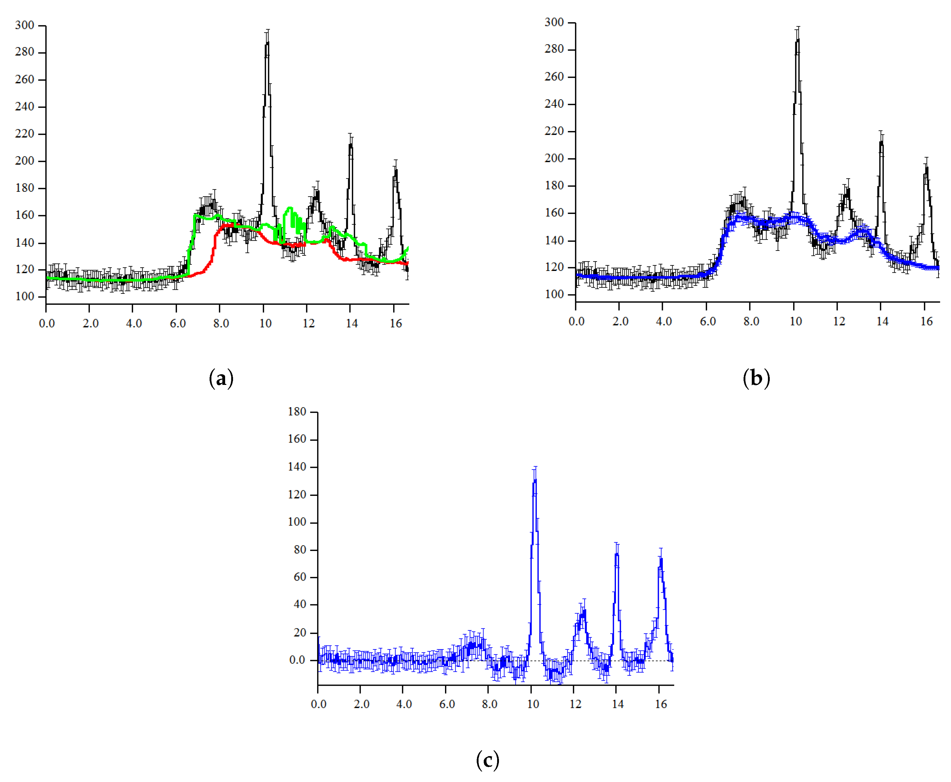
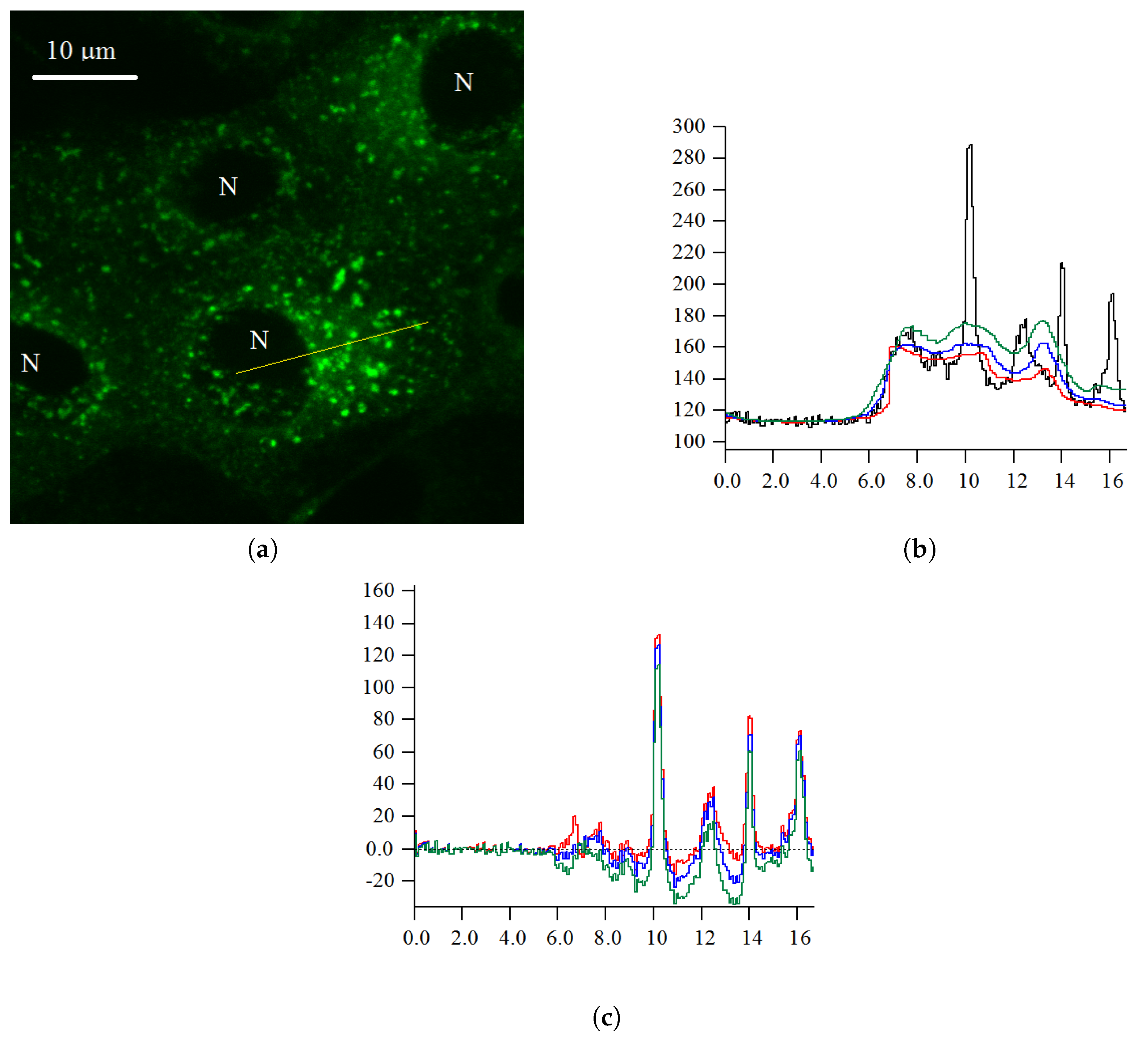
2. Two Background Level Estimation (TBL) Algorithm

2.1. Probabilistic Model of Intensity

Images of fluorescence microscopy are dominated by Poisson noise of photo-electron flux in photomultiplier tube (PMT) or CMOS/CCD camera. Probability to detect n photo-electrons is $P\left(n\right)=\frac{{\lambda }^n{e}^{-\lambda }}{\Gamma (n+1)}$. Assuming that intensity I linearly depends on number photo-electrons, we got $I=\alpha ·n+I_0$, where offset $I_0$ can be as positive as negative, dependent on microscope settings. Therefore, variance of intensity ${\sigma }^2=\alpha ·I+\zeta$, where $\zeta ={\epsilon }^2-\alpha ·I_0$ and ${\epsilon }^2$ is variance of zero-mean Gaussian noise of electronic circuits.

First, we found parameters $\alpha$ and $\zeta$ for a single image as it was described in [11]. In most practical cases ${\epsilon }^2$ is small, therefore we approximated $I_0=-\frac{\zeta }{\alpha }$ and subtracted it form the image: $J_i=max\left(0,I_i+\frac{\zeta }{\alpha }\right)$. Second, we calculated estimation of variance ${\sigma }_i^2$ for each pixel. Third, we approximated Poisson noise distribution by truncated Gaussian distribution (since it allows get integrals analytically):

Therefore, probability of intensity in absence of foreground, given background intensity $B_i$, was approximated as:

$$P\left(J_i|B_i,{\sigma }_i\right)=\sqrt{\frac{2}{\pi }}\frac{e^{-\frac{1}{2}\frac{{\left(J_i-B_i\right)}^2}{{\sigma }_i^2}}}{{\sigma }_i\left(-\frac{1}{\sqrt{2}}\frac{B_i}{{\sigma }_i}\right)},B_i\ge 0$$

(1)

In presence of foreground signal $F_i$ it was approximated as:

$$P\left(J_i,{\sigma }_i|B_i\right)={\int }_0^{\infty }\sqrt{\frac{2}{\pi }}\frac{e^{-\frac{1}{2}\frac{{\left(J_i-F_i-B_i\right)}^2}{{\sigma }_i^2}}}{{\sigma }_{i}erfc\left(-\frac{1}{\sqrt{2}}\frac{B_i}{{\sigma }_i}\right)}P\left(F_i\right)d{F}_i,$$

(2)

where $P\left(F_i\right)$ is prior of foreground. By maximum entropy principle, we chose prior distribution for foreground

$$P\left(F_i|{\mu }_i\right)=\frac{1}{\mu }{e}^{-\frac{F_i}{\mu }}$$

(3)

The parameter of the prior (mean expected amplitude of foreground$\mu$) was found outside of the analyzed pixel (see Appendix A).

After substitution (3) to (2) we got :

$$P\left(J_i,{\sigma }_i|B_i\right)=\frac{1}{\mu }\frac{e^{-\frac{1}{2}\frac{{\left(J_i-B_i\right)}^2}{{\sigma }_i^2}}}{\Psi \left(\frac{{\sigma }_i}{\mu }-\frac{J_i-B_i}{{\sigma }_i}\right)}\frac{e^{\frac{1}{2}{\left(\frac{B_i}{\sigma }\right)}^2}\Psi \left(\frac{{\sigma }_i}{\mu }+\frac{B_i}{{\sigma }_i}\right)\Psi \left(-\frac{B_i}{{\sigma }_i}\right)}{\Psi \left(\frac{{\sigma }_i}{\mu }+\frac{B_i}{{\sigma }_i}\right)+\Psi \left(-\frac{B_i}{{\sigma }_i}\right)},$$

(4)

where $\Psi \left(x\right)=\sqrt{\frac{2}{\pi }}\frac{e^{-\frac{1}{2}{x}^2}}{erfc\left(\frac{1}{\sqrt{2}}x\right)}$

2.2. Probabilistic Model of Two Background Levels

Assuming that background is slow varying signal, we approximate it by constant in the vicinity of the pixel i. The vicinity window is defined by characteristic scale discriminating background and foreground. We introduced latent variables $z_{i,k},k=1,2,3,4$ to define 4 possible states of pixel intensity: background B${}_1$, background B${}_2$, background B${}_1$ with foreground and background B${}_2$ with foreground. Then probability of intensities in the vicinity window $\Omega$ In the pixel having two background levels in the vicinity window, the probability of intensities we got:

$P\left(\left\{J_i,z_i\right\}|B_1,B_2,\left\{{\sigma }_i\right\}\right)=$

$$=\prod _{i\in \Omega }^{}{e}^{-\frac{1}{2}\frac{J_i^2}{{\sigma }_i^2}}\left(\begin{array}{c}{e}^{\frac{J_i{B}_{i,1}}{{\sigma }_i^2}}\Psi \left(-\frac{B_{i,1}}{{\sigma }_i}\right)\left(\frac{{\delta }_{z_i,1}}{{\sigma }_i}\left(1-{\beta }_0\right)+\frac{{\delta }_{z_i,2}}{\mu }\frac{{\beta }_0}{\Psi \left(\frac{{\sigma }_i}{\mu }-\frac{J_i-B_{i,1}}{{\sigma }_i}\right)}\frac{\Psi \left(\frac{{\sigma }_i}{\mu }+\frac{B_{i,1}}{{\sigma }_i}\right)}{\Psi \left(\frac{{\sigma }_i}{\mu }+\frac{B_{i,1}}{{\sigma }_i}\right)+\Psi \left(-\frac{B_{i,1}}{{\sigma }_i}\right)}\right)+\hfill \\ +e^{\frac{J_i{B}_{i,2}}{{\sigma }_i^2}}\Psi \left(-\frac{B_{i,2}}{{\sigma }_i}\right)\left(\frac{{\delta }_{z_i,3}}{{\sigma }_i}\left(1-{\beta }_0\right)+\frac{{\delta }_{z_i,4}}{\mu }\frac{{\beta }_0}{\Psi \left(\frac{{\sigma }_i}{\mu }-\frac{J_i-B_{i,2}}{{\sigma }_i}\right)}\frac{\Psi \left(\frac{{\sigma }_i}{\mu }+\frac{B_{i,2}}{{\sigma }_i}\right)}{\Psi \left(\frac{{\sigma }_i}{\mu }+\frac{B_{i,2}}{{\sigma }_i}\right)+\Psi \left(-\frac{B_{i,2}}{{\sigma }_i}\right)}\right)\hfill \end{array}\right)$$

(5)

where ${\beta }_0$ is prior probability of presence of foreground in the pixel (see Appendix A). If $\frac{B}{\sigma }>1$ , then the expression can be simplified as:

$P\left(\left\{J_i,z_i\right\}|B_1,B_2,\left\{{\sigma }_i\right\}\right)=$

$$=\prod _{i\in \Omega }^{}{e}^{-\frac{1}{2}\frac{J_i^2}{{\sigma }_i^2}}\left(\begin{array}{c}{e}^{\frac{J_i{B}_{i,1}}{{\sigma }_i^2}}\Psi \left(-\frac{B_{i,1}}{{\sigma }_i}\right)\left(\frac{{\delta }_{z_i,1}}{{\sigma }_i}\left(1-{\beta }_0\right)+\frac{{\delta }_{z_i,2}}{\mu }{\beta }_0\frac{1}{\Psi \left(\frac{{\sigma }_i}{\mu }-\frac{J_i-B_{i,1}}{{\sigma }_i}\right)}\right)+\hfill \\ +e^{\frac{J_i{B}_{i,2}}{{\sigma }_i^2}}\Psi \left(-\frac{B_{i,2}}{{\sigma }_i}\right)\left(\frac{{\delta }_{z_i,3}}{{\sigma }_i}\left(1-{\beta }_0\right)+\frac{{\delta }_{z_i,4}}{\mu }{\beta }_0\frac{1}{\Psi \left(\frac{{\sigma }_i}{\mu }-\frac{J_i-B_{i,2}}{{\sigma }_i}\right)}\right)\hfill \end{array}\right)$$

(6)

We used EM algorithm to maximize likelihood $L\left(B_1,B_2|\left\{J_i,z_i\right\},\left\{{\sigma }_i\right\}\right)$ over backgrounds$B_1,B_2$. Resulting backgrounds are presented on Figure 2a.

Then we calculated probability of presence of foreground in the pixel i (assuming $B_2>B_1$without loss of generality):

$$p_i^{signal}=\left\{\begin{array}{c}\frac{p_{i,z_i=4}}{p_{i,z_i=4}+p_{i,z_i=3}},I_i>B_2\hfill \\ \frac{p_{i,2}}{p_{i,z_i=2}+p_{i,z_i=1}}\hfill \end{array}\right.$$

(7)

where

$$p_{i,z_i=1}=\frac{\left(1-{\beta }_0\right)}{{\sigma }_i}{e}^{\frac{J_i{B}_{i,1}}{{\sigma }_i^2}}\Psi \left(-\frac{B_{i,1}}{{\sigma }_i}\right);p_{i,z_i=3}=\frac{\left(1-{\beta }_0\right)}{{\sigma }_i}{e}^{\frac{J_i{B}_{i,2}}{{\sigma }_i^2}}\Psi \left(-\frac{B_{i,2}}{{\sigma }_i}\right)$$

(8)

$$p_{i,z_i=2}=\frac{{\beta }_0}{\mu }\frac{e^{\frac{J_i{B}_{i,1}}{{\sigma }_i^2}}\Psi \left(-\frac{B_{i,1}}{{\sigma }_i}\right)\Psi \left(\frac{{\sigma }_i}{\mu }+\frac{B_{i,1}}{{\sigma }_i}\right)}{\Psi \left(\frac{{\sigma }_i}{\mu }-\frac{J_i-B_{i,1}}{{\sigma }_i}\right)\left(\Psi \left(\frac{{\sigma }_i}{\mu }+\frac{B_{i,1}}{{\sigma }_i}\right)+\Psi \left(-\frac{B_{i,1}}{{\sigma }_i}\right)\right)}$$

(9)

$$p_{i,z_i=4}=\frac{{\beta }_0}{\mu }\frac{e^{\frac{J_i{B}_{i,2}}{{\sigma }_i^2}}\Psi \left(-\frac{B_{i,2}}{{\sigma }_i}\right)\Psi \left(\frac{{\sigma }_i}{\mu }+\frac{B_{i,2}}{{\sigma }_i}\right)}{\Psi \left(\frac{{\sigma }_i}{\mu }-\frac{J_i-B_{i,2}}{{\sigma }_i}\right)\left(\Psi \left(\frac{{\sigma }_i}{\mu }+\frac{B_{i,2}}{{\sigma }_i}\right)+\Psi \left(-\frac{B_{i,2}}{{\sigma }_i}\right)\right)}$$

(10)

Assuming that each pixel in the vicinity window exclusively belongs to only one background level, we got probability of background levels: Assuming that each pixel in the vicinity window exclusively belongs to only one background level, we got probability of background levels:

$$P_{j,1}=\sum _{i=1}^N\left(\left(p_{i,1}+p_{i,2}\right)·p_i^{signal}·p_j^{signal}+p_{i,1}·\left(1-p_i^{signal}·p_j^{signal}\right)exp\left(-\frac{{\left(I_i-I_j\right)}^2}{2\left({\sigma }_i^2+{\sigma }_j^2\right)}\right)\right)$$

(11)

$$P_{j,2}=\sum _{i=1}^N\left(\left(p_{i,3}+p_{i,4}\right)·p_i^{signal}·p_j^{signal}+p_{i,3}·\left(1-p_i^{signal}·p_j^{signal}\right)exp\left(-\frac{{\left(I_i-I_j\right)}^2}{2\left({\sigma }_i^2+{\sigma }_j^2\right)}\right)\right)$$

(12)

Finally consensus background intensity in the pixel of interest was calculated as weighted mean:

$$B=\frac{B_1{P}_1+B_2{P}_2}{P_1+P_2}$$

(13)

The estimation of variance of background intensity:

$${\sigma }_b^2=Va{r}_{B_1}{\left(\frac{P_1}{P_1+P_2}\right)}^2+Va{r}_{B_2}{\left(\frac{P_2}{P_1+P_2}\right)}^2+{\left(B_1-B_2\right)}^2\frac{P_1{P}_2}{{\left(P_1+P_2\right)}^2}\frac{1}{N}$$

(14)

Final background was calculated by formula (14) (Figure 2b). Difference between original intensities and estimated backgrounds has residual “nuclei border artifact” within estimated uncertainty (Figure 2c).

Result of TBL algorithm is presented on Figure 3a,b.

3. Conclusions

We developed a new algorithm (TBL) to estimate cytoplasm fluorescence (background) in conditions where high spatial frequency is present in both background and foreground signal. TBL avoids artefacts that are characteristic for state-of-the-arts background subtraction algorithms in presence inhomogeneous background with sharp transition between levels.

References

1. Zimmer, M. Green Fluorescent Protein (GFP): Applications, Structure, and Related Photophysical Behavior. Chem. Rev. 2002, 102, 759–782. [Google Scholar] [CrossRef] [PubMed]
2. Rink, J.C.; Ghigo, E.; Kalaidzidis, Y.L.; Zerial, M. Rab Conversion as a Mechanism of Progression from Early to Late Endosomes. Cell 2005, 122, 735–749. [Google Scholar] [CrossRef] [PubMed]
3. Meijering, E.; Smal, I.; Danuser, G. Tracking in Molecular Bioimaging. IEEE Signal Process. Mag. 2006, 23, 46–53. [Google Scholar] [CrossRef]
4. Sbalzarini, I.F.; Koumoutsakos, P. Feature point tracking and trajectory analysis for video imaging in cell biology. J. Struct. Biol. 2006, 151, 182–195. [Google Scholar] [CrossRef] [PubMed]
5. Pfeffer, S.R. Rab GTPases: master regulators that establish the secretory and endocytic pathways. Mol. Biol. Cell 2017, 28, 712–715. [Google Scholar] [CrossRef] [PubMed]
6. Pécot, T.; Bouthemy, P.; Boulanger, J.; Chessel, A.; Bardin, S.; Salamero, J.; Kervrann, C. Background Fluorescence Estimation and Vesicle Segmentation in Live Cell Imaging with Conditional Random Fields. IEEE Trans. Image Process. 2015, 24, 667–680. [Google Scholar] [CrossRef] [PubMed]
7. Kalaidzidis, Y. (Version 8.93.00, 27 June 2019). Available online: http://motiontracking.mpi-cbg.de.
8. Lee, H.-C.; Yang, G. Computational Removal of Background Fluorescence for Biological Fluorescence Microscopy. In Proceedings of the IEEE 11th International Symposium on Biomedical Imaging (ISBI), Beijing, China, 29 April–2 May 2014. [Google Scholar]
9. Yang, L.; Zhang, Y.; Guldner, I.H.; Zhang, S.; Chen, D.Z. Fast Background Removal in 3D Fluorescence Microscopy Images Using One-Class Learning. In International Conference on Medical Image Computing and Computer-Assisted Intervention—ICCAI 2015, Part III; Springer: Cham, Switzerland, 2015; pp. 292–299. [Google Scholar]
10. Sternberg, S.R. Biomedical Image Processing. Computer (IEEE) 1983, 16, 22–34. [Google Scholar] [CrossRef]
11. Kalaidzidis, Y. Fluorescence Microscopy Noise Model: Estimation of Poisson Noise Parameters from Snap-Shot Image. In Proceedings of the International Conference on Bioinformatics and Computational Biology (BIOCOMP’17), Las Vegas, NV, USA, 17–20 July 2017; pp. 63–66. [Google Scholar]
Figure 1. (a) A431 cells with GFP-tagged Rab5a. The cytosol is labelled by soluble fraction of GFP-Rab5a. Bright structures of different size and shape are endosomes, which are labelled by membrane-bound GFP-Rab5a. Images were obtained by spinning disk microscope (Andor-Olympus-IX71 inverted stand microscope; scan head CSU-X1 Yokogawa, objective Olympus UPlanSApo 63x 1.35oil, Optovar 1.6). Letters N denote nuclei. Yellow line marks the intensity profile presented on panel b. (b) Intensity profiles along the yellow line (Figure 1). Black curve is intensity of original image. Red, green, blue and cyan curves are background estimation by “rolling ball” [10], Gaussian, median and FMOR [7] filters respectively. (c) Difference between original intensities and estimated background. Green, blue and red curves correspond to background estimation by Gaussian, median and FMOR filters respectively. Filter window was 4 μ m for all filters.
Proceedings 33 00022 g001
Figure 2. (a) Original intensity (as on Figure 1) curve (black) and two estimated background levels (red and green curves). (b) Original intensity curve (black) and background estimation by TBL (blue) curve. (c) Difference between original intensities and TBL background.
Proceedings 33 00022 g002
Figure 3. (a) Original image. (b) Image after subtraction background by TBL.
Proceedings 33 00022 g003