A Study on the Behavior of Clustering Techniques for Modeling Travel Time in Road-Based Mass Transit Systems ^†

Abstract

In road-based mass transit systems, the travel time is a key factor affecting quality of service. For this reason, to know the behavior of this time is a relevant challenge. Clustering methods are interesting tools for knowledge modeling because these are unsupervised techniques, allowing hidden behavior patterns in large data sets to be found. In this contribution, a study on the utility of different clustering techniques to obtain behavior pattern of travel time is presented. The study analyzed three clustering techniques: K-medoid, Diana, and Hclust, studying how two key factors of these techniques (distance metric and clusters number) affect the results obtained. The study was conducted using transport activity data provided by a public transport operator.

1. Introduction

The current paradigm of Intelligent Transport Systems is based on the continuous observation of what happens in the transport network to achieve safer transport systems, more environmentally friendly, more efficient, and focused on the needs of users [1]. This is possible thanks to technological advances in sensors, communications, and computing. In this context, Data Science and, more specifically, Data Mining and Big Data are increasingly referenced in the development of intelligent transport systems.

Travel time (TT) is a critical aspect of transportation systems. In general, planners try to minimize this time, avoiding its variability. In the case of road-based mass transit systems, TT becomes more relevant because this time is used as a metric to evaluate the quality of service. The work described in this contribution has been developed in the context of road-based mass transit systems. Its objective was the study of TT. Specifically, this article presents a study about the utility of different clustering techniques to obtain behavior pattern of TT. The aim has been to analyze the potential of these techniques to obtain TT patterns that generate knowledge applicable to key aspects in this type of transport system, such as the case of short-term forecasting or long-term estimation of TT used in the services scheduling. The main contributions of this work are first, the study of three representative clustering techniques to obtain knowledge about TT, and second, the methodology followed has permitted to analyze how the main aspects of the tested clustering techniques affect the results obtained.

This document is structured as follows: next, related works are presented, the methodology followed is described in the third section, the results and their discussion are presented in the fourth section, and finally, the main conclusions and future works are presented in the fifth section.

2. Related Works

The use of Data Science to improve transport systems and especially public transport systems is an increasingly frequent topic in the bibliography. This section is focused on road-based mass transit systems and, more specifically, on those works related to TT. In this specific context, there is a wide bibliography of works about the short-term prediction of TT, meaning short-term prediction are those that are made in a vehicle to estimate the TT required to cover a segment of the route that is being made. The models proposed for this type of forecasting are used in the operations control systems of public transport operators, the objective of these systems is to guarantee the timetables’ adherence. Moreira-Matias et al. [2] conduct a comprehensive review of techniques used for this type of prediction. Focusing on Machine Learning techniques, taking into account the type of technique used and the references number, we highlight Yu et al. [3] who proposed models based on support vector machines, Bai et al. [4] who proposed a combined model based on support vector machine and Kalman filters, Gurmu et al. [5] who presented a prediction model based on artificial neuronal networks, Chang et al. [6] who proposed the technique k-nearest neighbors, Gal et al. [7] that used decision tree regression and finally, the work of Lee et al. [8] that proposed clustering techniques, specifically K-means and V-means. All these short-term TT forecasting models use, as input data, a set of TT observed at different points in the transport network in certain instants in time. One shortcoming in these proposals is that the criteria used for the selection of this set of TT are not explained. Therefore, having a knowledge of the behavior of TT, which is the objective of this work, the selection of these input data can be improved, increasing the prediction accuracy.

In road-based mass transit systems, the long-term prediction of TT consists of estimating this time for different routes that are part of the line service scheduling. This prediction is important because the services scheduling and stops timetable are made considering these estimations. Mendes-Moreira et al. [9] analyze the behavior of three regression techniques: projection pursuit regression, support vector machine and decision trees based on random forest, taking as data for the study those provided by the biggest public road passenger transport operator in the city of Oporto, in the period from 1 January to 30 August 2004. The authors of this paper concluded that the prediction based on projection pursuit regression produced the best results. However, this technique requires a previous selection of parameters and a pre-processing of the input data. Therefore, the authors conclude that the prediction technique based on random forest is attractive because it produces comparable results without requiring prior processes. To provide knowledge about factors that affect to TT and thus, to be able to make better estimation, Comi et al. [10] conducted a study based on time series in the city of Rome, relating TT to traffic conditions, and Yetiskul and Senbil [11] related TT to temporal and spatial factors in the city of Ankara. Finally, Bie et al. [12] developed a clustering technique whose objective is the adequate partitioning of time of day to improve line services scheduling, the aims were to improve the punctuality and to cover the demand variations adequately. The work presented in this contribution is a complement to these works, due to the fact that once the TT patterns have been obtained, the existence of common factors can be analyzed, such as traffic conditions associated with types of day (calendar day, working day or holiday day), time slots (peak or off-peak day) and segments of the transport network that affect this time.

3. Methodology

Knowing how a certain variable affects the quality of the product or service is an important aspect for organizations. Nowadays, because of technological advances in computing, sensors and mobile communications, most of the activities, carried out in organizations or carried out by its clients, produce data that allow obtaining interesting traces of activities or behaviors, and make possible the evaluation of the quality of service provided by corporations. Data Mining is a discipline that provides techniques that allow obtaining this knowledge; its objective is to obtain useful knowledge from the data. In this context, useful knowledge means to be able to predict the value of a variable or to identify which factors affect its behavior. The study presented in this paper aims to analyze different clustering techniques for obtaining useful knowledge about TT. This study focuses on clustering techniques because they are unsupervised methods, allowing us to find hidden behavior patterns in large data sets.

3.1. TT conceptualization

TT is a key factor in the quality of service in public transport. The users want their travel times to be short and predictable. In addition, they want maximum adherence to timetables offered by public transport operators. For a route of a line service, the TT from the stop origin of the route to the n-th stop can be expressed according to Formula (1). In this formula, DT_n is the time invested by passengers in getting on or off the vehicle at stop n, this is called dwell time, and it is a time in which the vehicle is stopped. Rt_n is the time the vehicle spends going from one stop to the next on the planned route. During this time, the vehicle may be in motion or stopped due to a traffic signal or traffic conditions. This is called nonstop running time. Therefore, TT is affected by traffic conditions, traffic signs, and mobility patterns of public transport users.

$$TT=\sum _{n=1}^N{DT}_n+\sum _{n=1}^{N-1}{RT}_n.$$

To obtain the TT on the route of a public transport line service, there are two basic data sources: automatic vehicle location systems (AVL) and automatic vehicle passenger counting systems (APC). With APC, the TT is obtained from the records of passenger boarding and alighting in vehicles. In the case of AVL, two scenarios are possible. In the first scenario, the systems specifically record the instant of time in which the vehicle arrives at each stop on the route, then the TT at each stop can be obtained from this record. The second scenario occurs when the instant of arrival is not specifically recorded, then this time must be obtained from a reconstruction of the route, the accuracy of which will depend on the frequency with which the vehicle’s positioning readings are taken. In the study presented, the TT data were obtained from the positions of the vehicles, using a reconstruction of the routes carried out with the GPS readings, with a frequency of one minute.

3.2. Representation of the TT

Since the objective of this study is to know the behavior of the TT in the different routes of the transport network, the entities to be classified are made up of the TT observed in a set of stops selected from each route, during the expeditions carried out in a significant time interval. If n stops have been selected in a route then, for the purposes of this study, each expedition will be represented by a n-tuple (TT₁, ... TT_n) in which each TT_i is the TT observed in the expedition at the i-n stop, measured with respect to the scheduled start time of the line service. The selection of the stops in the different routes was carried out considering two criteria: stops that were used by a greater number of passengers and stops located at a similar distance from the next one. Table 1 shows the data structure used to represent the TT entity observed for a route on a line, where, in addition to the n-tuple mentioned above, the observed start time of the line service, called T₀, was recorded, for the subsequent analysis phase.

Table 1. Structure of travel time (TT) record.

TT0

TT1

TT2

...

TTn

Figure 1 shows a graphical representation of a set of TT records for a given route in which five stops, that is four segments, have been selected. The stops are represented on the horizontal axis. On the vertical axis, the TT is observed, and each grey graph is the representation of one of the routes of the line.

Figure 1. Illustration of travel time (TT) records clustering with five stops.

3.3. Clustering Techniques

Clustering is a family of unsupervised machine learning techniques, aimed to search for patterns in the observations of a given phenomenon. These techniques group the observations into different sets so that all the observations belonging to the same set are similar. Therefore, metrics that measure the similarity between observations play a main role in clustering techniques. These techniques can be classified into three groups:

• Techniques based on partitioning the set of observations into several clusters initially specified.
• Hierarchical techniques, in which it is not necessary to specify the number of clusters.
• Methods combining the above techniques.

The objective of this study is to evaluate the usefulness of different clustering techniques for obtaining intelligible patterns on the behavior of the TT. In this context, intelligibility means the ability to interpret these patterns in such a way that they provide useful knowledge that can be used when scheduling line services. The study analyzed the behavior of three clustering techniques: the partitioning technique K-medoids (based on the Pam Algorithm) [13], and two hierarchical techniques: Diana (a divisive method) [14] and Hclust (an agglomerative method) [15], using Euclidean distance and Manhattan distance as similarity metrics. The average value of the Silhouette function [16] was used to analyze the optimal number of clusters for each technique.

3.4. Phases of the Methodology

As expressed in Section 3.2, the entities to be classified are the observed TT on the line services of a route named expeditions. If L represents the line route to be analyzed and T the time when the TT analysis was carried out, then the set of all the expeditions of L that were carried out during the T period is represented by E_L,T. Based on this notation, the methodology followed in this study can be described as follows:

• Phase 1. Given a route and a period, generate the whole E_L,T from coherent and quality positioning records of the expeditions carried out in that period.
• Phase 2. Creation of the clusters, applying each of the clustering techniques indicated to the E_L,T set, and selection of the optimum number of clusters.
• Phase 3. Representation of results to evaluate the new information obtained.
• Phase 4. Analysis of the results obtained.

4. Results and Discussion

The methodology was applied to analyze the TT of a public transport line on the island of Gran Canaria. This line has 42 stops and a length of just over 30 km in the central corridor of the island. From the point of view of passenger movement, this corridor mainly travels along regional roads linking two important rural centers with the capital of the island. Figure 2 shows a map of the route and the stops on the line.

Figure 2. Route and stops of the analyzed line.

In terms of resources and tools, a computer with an Intel(R) Core (TM) i7-2600K CPU processor @ 3.40 GHz with 16 GB RAM was used. Oracle DB—the database environment used by the transport operator that provided its data—was used to prepare the data. For the Clustering techniques analysis, the RStudio framework was used, specifically the packages Cluster [17] and Factoextra [18]. To visually map the data, the GoogleMap framework was used. Each of the tasks carried out in the experimental phase is described in detail below.

4.1. Phase 1: Generation of the set E_L,T

The period T used in this study was the whole year 2015. The expeditions of the line analyzed in this period were reconstructed from the GPS positions registered in the vehicles, to obtain the TT at every selected stop, generating the n-tuples of values that were stored in the register represented in Table 1, and constituting the set E_L,T. The GPS readings were taken with a frequency of one minute. Table 2 shows the total number of GPS readings obtained in the analyzed expeditions (row NGPS), the total number of reconstructed expeditions of the analyzed route (row NEXP) and the total number of reconstructed expeditions that passed the validation process to guarantee the integrity of the data set used in the study (row NCEXP). This validation consisted of discarding erroneous or poor-quality GPS readings and expeditions whose reconstructed routes were not consistent with the planned route.

Table 2. Number of GPS readings (NGPS), number of reconstructed expeditions (NEXP), and number of validated expeditions (NCEXP).

NGPS	615.813
NEXP	9.887
NCEXP	7.862

4.2. Phase 2: Creation of the Clusters and Determination of Their Optimum Number

The goal of this phase is to know which combination of clustering technique, metric distance, and number of the clusters allows better discovery behavior patterns of the TT that provide new intelligible information. Therefore, once the E_L,T set was generated, each clustering technique mentioned above was executed using alternatively two similarity metrics (Euclidean distance and Manhattan distance) and different clusters number, from 2 to 5, generating between 2 and 5 patterns (a number greater than 5 patterns would complicate the subsequent analysis phase). The function Silhouette was used to evaluate the quality of the resulting clustering. The average Silhouette obtained in each case, that is, each combination of clustering technique, similarity metric, and clusters number is shown in Figure 3. The clusters number used in each clustering process is represented in the horizontal axis. The average Silhouette obtained in each clustering process is represented in the vertical axis. Each curve represents a cluster technique (K-medoid using pam algorithm, hierarchical clustering using Diana algorithm, and hierarchical clustering using Hclust) using a similarity metric (Euclidean distance or Manhattan distance).

Figure 3. Average silhouette obtained in each of the groupings performed.

Table 3 presents the elapsed CPU time, in seconds, for each combination of clustering technique, distance, and clusters number.

Table 3. Elapsed CPU times in seconds for each clustering performed.

	Number of Clusters
	2	3	4	5
pam-manhattan	8.35	4.07	15.8	10.39
pam-euclidea	7.15	4.21	11.62	13.27
hclust-manhattan	4.61	3.92	3.88	3.94
hclust-euclidea	3.93	4	3.89	3.9
diana-manhattan	1235.68	1238.88	1272.35	1279.8
diana-euclidea	1317.6	1390.47	1387.73	1278.11

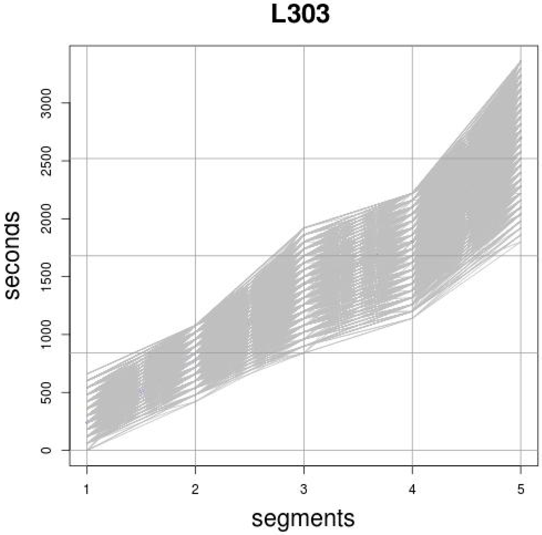
4.3. Phase 3: Results Representation

This phase produced two results. On the one hand, the generated TT patterns, determined by their representative elements, that were centroids, and on the other hand, the start instant (date and time of day) of the expeditions belonging to the same cluster. To represent this second result intelligibly, the technique was the Heatmaps Graph. This technique allows, using color palettes, the values contained in an array to be shown. In this case, in which the goal is to analyze the new information contained in the records included in each cluster, the matrix was determined by the proportion of records contained in certain time intervals related to the month, week day, and the time of day. The color palette selected to represent each cluster goes from white to the colour assigned to each one (red for cluster 1, blue for cluster 2,...) in such a way that, a cell of light color means that there were few registers with those temporal characteristics in the cluster, and the intense color means that there were many registers with those characteristics in the cluster.

4.4. Phase 4: Analysis of Results

The following conclusions can be drawn from the average values resulting from the Silhouette function shown in Figure 3. First, the Manhattan distance was the most convenient in the clustering techniques applied (represented by the continuous lines). Second, the quality of the clusters created by the K-medoids and Diana algorithms was similar when dealing with two clusters (0.458 and 0.461, respectively). Using three clusters, k-medoids had a higher value (0.394 vs. 0.352). Using four or five clusters, the quality of the clusters generated by the Diana exceeded those created by the K-medoids. This is due to the hierarchical divisive Diana method, which can quickly isolate the elements with the greatest deviation from the whole, resulting in clusters less compensated, in terms of total elements, but more compact. This effect can be observed in Figure 4, where the four clusters generated by both algorithms are presented. Observe that cluster 2 stands out with only 142 registers, but which made clusters 3 and 4 more compact and have a higher Silhouette value.

Figure 4. Clusters generated with four clusters with (a) Diana; (b) K-medoids.

To evaluate the convenience of the clustering methods, the time required to execute each clustering technique is another relevant issue, especially if the techniques were applied to the entire transport network. The elapsed CPU times presented in Table 3 show that the Diana clustering method was the one that required the most CPU time. It spent 100 times more processor in the best of cases.

To analyze the relationship between the elements of each cluster and temporal variables, two different heatmaps were generated. The first, relating the registers belonging to each cluster to the pair of temporal attributes (month of the year, day of the week), see Figure 5. The second, relating the registers belonging to each cluster to the pair (day of the week, time of the day), see Figure 6. In both figures, there are well-differentiated stripes that reflect the occurrence of TT patterns in these periods of time. Figure 6 shows a similar behavior of the patterns identified throughout the year, highlighting, for example, the lowest TT on Sundays and Saturdays throughout the year. Figure 6 shows in greater detail the behavior at different times of the day, where higher values of TT were observed on late Friday and Saturday expeditions, conditioned by the greater influx of passengers and their times for getting on or off the vehicles.

Figure 5. Heatmaps of k-medoids with two clusters showing the relation of their records with the months of the year and the days of the week.

Figure 6. Heatmaps of k-medoids with two clusters, showing the relation of their records with the days of the week and the hours of the day of the expeditions.

5. Conclusions

To make reliable service scheduling to improve service quality, TT plays a key role in road-based mass transit systems. For this reason, the methodology development for obtaining useful but not evident knowledge about TT is a relevant topic in this kind of transport system. Unsupervised methodologies that can use massive data related to transport activity are interesting, especially highlighting the clustering techniques since they allow two fundamental objectives in any process of knowledge discovery to be reached. First, to find patterns that characterize in the space or in the time the behavior of relevant factors in the transport activity (as they can be the travel times or the demand of the services). Second, these patterns can be represented in an intelligible way constituting a new resource for the operators or for the competent authorities.

To deepen in this type of process of extraction of new information, a study about the utility of different clustering techniques to obtain TT behavior pattern has been presented in this paper. The clustering techniques analyzed were K-medoid, which is a type of partitioning clustering technique, and the hierarchical techniques Diana and Hclust. The study evaluated these clustering methods and analyzed the usefulness of these to obtain intelligible information. Using real public transport data provided by an interurban transport company of Gran Canaria (Canary Islands, Spain), the results obtained have demonstrated that clustering techniques are useful to obtain useful knowledge about TT. Additionally, the influence of two key aspects in clustering techniques (similarity metric used and clusters number) in the results was analyzed. From this analysis it is concluded that first, the Manhattan distance is the most convenient in the clustering techniques applied; second, the quality of the clusters created by the K-medoids and Diana algorithms is similar when dealing with two or three clusters, but for a larger number of clusters, Diana behaves better. In addition, the time required to execute each clustering technique was another relevant issue evaluated. In this evaluation, the Diana clustering method was the one that required the most CPU time. It spent 100 times more processor time in the best of cases. Finally, to analyze the relationship between the elements of each cluster and temporal variables, two different heatmaps were generated. The first is related to the registers belonging to each cluster with the pair of temporal attributes (month of the year, day of the week). The second is related to the registers belonging to each cluster with the pair (day of the week, time of the day). In both cases, there were well-differentiated stripes that reflect the occurrence of TT patterns in these periods of time.

References

1. Zhang, J.; Wang, F.; Wang, K.; Lin, W.; Xu, X.; Chen, C. Data-driven intelligent transportation systems: A survey. IEEE Trans. Intell. Transp. Syst. 2011, 4, 1624–1639. [Google Scholar] [CrossRef]
2. Moreira-Matias, L.; Mendes-Moreira, J.; de Sousa, J.F.; Gama, J. Improving Mass Transit Operations by Using AVL-Based Systems: A Survey. IEEE Trans. Intell. Transp. Syst. 2015, 16, 1636–1653. [Google Scholar] [CrossRef]
3. Yu, B.; Yang, Z.; Yao, B. Bus Arrival Time Prediction Using Support Vector Machines. J. Intell. Transp. Syst. 2007, 10, 151–158. [Google Scholar] [CrossRef]
4. Bai, C.; Peng, Z.-R.; Lu, Q.-C.; Sun, J. Dynamic Bus Travel Time Prediction Models on Road with Multiple Bus Routes. Comput. Intell. Neurosci. 2015, 2015, 1–9. [Google Scholar] [CrossRef] [PubMed]
5. Gurmu, Z.K.; Nall, T.; Fan, W. Artificial Neural Network Travel Time Prediction Model for Buses Using Only GPS Data. J. Public Transp. 2007, 17, 45–65. [Google Scholar] [CrossRef]
6. Chang, H.; Park, D.; Lee, S.; Lee, H.; Baek, S. Dynamic multi-interval bus travel time prediction using bus transit data. Transportmetrica 2010, 6, 19–38. [Google Scholar] [CrossRef]
7. Gal, A.; Mandelbaum, A.; Schnitzler, F.; Senderovich, A.; Weidlich, M. Traveling time prediction in scheduled transportation with journey segments. Inf. Syst. 2017, 64, 266–280. [Google Scholar] [CrossRef]
8. Lee, W.-C.; Si, W.; Chen, L.-J.; Chen, M.C. http: A New Framework for Bus Travel Time Prediction Based on Historical Trajectories. In Proceedings of the International Conference on Advances in Geographic Information Systems (ACM SIGSPATIAL GIS 2012), California, CA, USA, 6–9 November 2012. [Google Scholar] [CrossRef]
9. Mendes-Moreira, J.; Mario Jorge, A.; Freire de Sousa, J.; Soares, C. Comparing state-of-the-art regression methods for long term travel time prediction. Intell. Data Anal. 2012, 16, 427–449. [Google Scholar] [CrossRef]
10. Comi, A.; Nuzzolo, A.; Brinchi, S.; Verghini, R. Bus travel time variability: Some experimental evidences. Transp. Res. Procedia 2017, 27, 101–108. [Google Scholar] [CrossRef]
11. Yetiskul, E.; Senbil, M. Public bus transit travel-time variability in Ankara (Turkey). Transp. Policy 2012, 23, 50–59. [Google Scholar] [CrossRef]
12. Bie, Y.; Gong, X.; Liu, Z. Time of day intervals partition for bus schedule using GPS data. Transp. Res. Part C 2015, 60, 443–456. [Google Scholar] [CrossRef]
13. Kaufman, L.; Rousseeuw, P.J. Partitioning around medoids (program PAM). In Finding Groups in Data Finding Groups in Data: An Introduction to Cluster Analysis; Kaufman, L., Rousseeuw, P.J., Eds.; Wiley: Hoboken, NJ, USA, 2009; pp. 68–125. [Google Scholar] [CrossRef]
14. Kumar-Patnaik, A.; Kumar-Bhuyan, P.; Krishna-Raob, K.V. Divisive Analysis (DIANA) of hierarchical clustering and GPS data for level of service criteria of urban streets. Alex. Eng. J. 2016, 55, 407–418. [Google Scholar] [CrossRef]
15. Murtagh, F.; Legendre, P. Ward’s Hierarchical Agglomerative Clustering Method: Which Algorithms Implement Ward’s Criterion? J. Classif. 2014, 31, 274–295. [Google Scholar] [CrossRef]
16. Rousseeuw, P.J. Silhouettes: A graphical Aid to the Interpretation and validation of Cluster Analysis. J. Comput. Appl. Math. 1987, 20, 53–65. [Google Scholar] [CrossRef]
17. Cluster Analysis Basics and Extensions. R Package Version 2.0.6. Available online: https://CRAN.R-project.org/package=cluster (accessed on 28 June 2019).
18. Factoextra: Extract and Visualize the Results of Multivariate Data Analyses. R Package Version 1.0.5. Available online: https://CRAN.R-project.org/package=factoextra (accessed on 28 June 2019).
Publisher’s Note: MDPI stays neutral with regard to jurisdictional claims in published maps and institutional affiliations.
Article Metrics
Citations
Article Access Statistics
Multiple requests from the same IP address are counted as one view.