1. Introduction
To increase building energy efficiency, smart control strategies such as model predictive control (MPC) have been gaining a lot of interest recently [
1]. Different studies revealed that advanced control of HVAC&R systems has the potential to produce energy savings compared to more traditional control strategies such as PIDs and rulebased controllers [
1]. Additionally, these control strategies are particularly well suited for demand side or peak demand management. An example of such system who could benefit from predictive control are domestic hot water (DHW) systems. For example, it was found in [
2] that a predictive controller could provide energy savings around 5% when applied to a DHW heating system compared to a reference control strategy.
To better manage the energy consumption of a water heating system while providing enough DHW to the occupants and respecting the system’s constraints [
3], an MPC could optimize the water flowrate supplied to the water heater, the amount of hot water stored in the tank, and the water heater temperature setpoint. In order to do so, the MPC requires predictions of the future DHW demand over a given prediction horizon. These predictions are produced by a predicting model that can either be a white box model (e.g., based on the physics of the system), a black box model (e.g., based on machine learning strategies), or a grey-box model (e.g., a mix of white and black box models) [
4].
The purpose of the present work is to develop a predicting model for DHW demand with the help of a recurrent neural network (RNN) (i.e., black box model). As mentioned above, such model could eventually be used in a predictive controller.
2. Case-Study
The DHW consumption of a 40 unit residential building in Quebec City, Canada, has been measured every 10 min from October 2015 to August 2018. This corresponds to a dataset of 132,600 points, approximately.
The DHW system can be considered as centralised (i.e., a water heater and hot water tanks supplying the whole building), thus only the total consumption of the building is considered here. The total volume of the tanks is 1800 L and the available effective heat transfer rate is 300 kW.
3. DHW Consumption Profile
In order to demonstrate the necessity of using an advanced predicting method, such as the one developed in this work, instead of hourly demand schedules such as those proposed for energy simulations, for example by ASHRAE [
5], the DHW demand distribution is first analyzed.
Given the average demand value of 247.38 L/h and the standard deviation of 262.2 L/h, it is clear that the values are spread over a large interval of possible values, and, thus, could prove difficult to predict from a schedule.
The hourly DHW demand has been averaged for every hour of the day throughout the entire measured dataset and is reported in
Figure 1 as a function of the time of the day. From the analysis of the standard deviation (σ), it can be seen that the total water consumption of the case-study building varies significantly from day-to-day. Thus a static schedule is not adequate to produce accurate predictions and a more advanced predicting model is developed in the following section.
4. Predicting Future DHW Demand
To predict the total DHW demand during the next time step of 10 min, a recurrent neural network (RNN) is trained using the measured data from the case-study building. More precisely, an RNN is a “family of neural networks for processing sequential data” [
6]. It is recurrent because each hidden layer has a recurrent connection, allowing it to remember information from previous states. They can be used for regression purposes for time-series data, such as predicting the next DHW demand.
The selected RNN inputs for the prediction of the next DHW demand are as follows: (1) year, (2) month of the year, (3) day of the month, (4) day of the week, (5) hour of the day and (6) current DHW demand. The year where the measurement is made is considered to affect the DHW demand since it is a residential building (apartments) and occupants can vary from year to year. In addition, the recurrence adds the information available from the five previous time steps. The prediction target value for the training of the RNN is the next measured demand (10 min later).
Based on the recommendations of [
7], the RNN is composed of two hidden layers containing 13 neurons each. Indeed, it is stipulated in [
7] that neural networks with two to three hidden layers can approximate any practical function. For the hidden layer size, it is usually recommended to have a minimum of 2n + 1 neurons per hidden layer [
8], where n is the amount of inputs. To reduce computational time and with six inputs, the smallest neural network is produced with two layers of 13 neurons each.
The neural network is trained using 106,250 measured data points, with 70%, 15%, and 15% of them used for the training, validating and testing of the RNN, respectively. To test the neural network’s ability to generalize to new data, the remaining values from the full dataset (around 25,000 data points) were used to form a second testing dataset. This corresponds to around six months of measured data from February to August. The duration of this testing dataset has been chosen in order to represent every aspects of the Canadian climate. This dataset is used to measure the performance indices presented in this work.
To avoid overfitting, the early stopping strategy is used in the training of the neural network (i.e., after six time steps where the validation error increases, the training is stopped and the selected weight values for the neural network are the ones associated with the minimal validation error) [
9].
In order to evaluate the predicting accuracy, two performance indices are evaluated between the measured and predicted data: (i) the root mean square error (RMSE) and (ii) the coefficient of determination (R2).
The values obtained by predicting the next demand using the designed RNN are an RMSE of 197.50 L/h and an R
2 of 0.43. The distribution of the predictions is presented in
Figure 2.
As can be seen in
Figure 2a, the RNN predicts small consumption with better accuracy than the high demands. Indeed, for demands over 900 L/h, the prediction quality degrades as the predictions are further away from the measured values.
Functions that fluctuate and vary rapidly such as the measured DHW demand can be difficult to predict. Indeed,
Figure 2b shows that the measured demand fluctuates with an important amplitude and the RNN has difficulties predicting the peak values. These rapid fluctuations will be referred to as “noise” for the remaining of this work, although they do not represent only unwanted modifications to the measurements and can potentially carry useful information. Nevertheless, it should be noted that this noise is introduced to a certain extent by the resolution of the cumulative water consumption sensors of the dwelling units. Indeed, the smallest measurable value is 10 L.
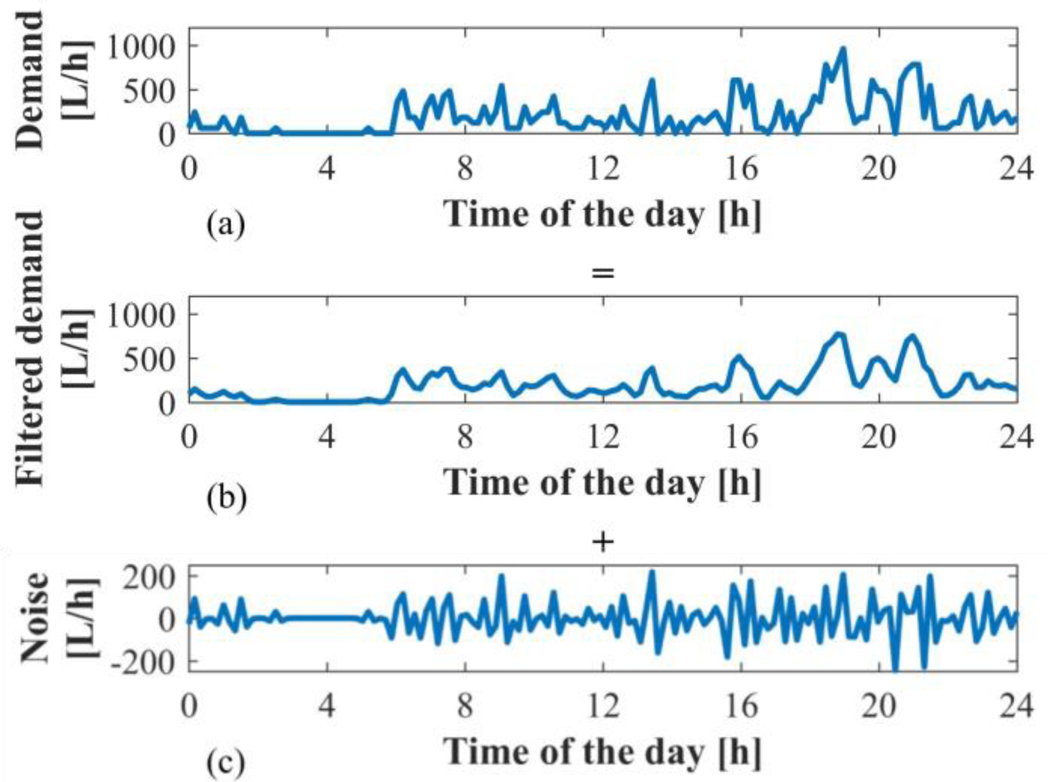
5. Predicting Noisy DHW Demand
To avoid the problems brought by the highly noisy component of the DHW demand signal, another strategy is to use a Gaussian filter to separate the noise from the demand. More specifically, Gaussian filters are commonly used with timeseries such as the DHW demand to smoothen the measured signal [
10]. The profiles obtained with this approach are shown in
Figure 3 for a selected day.
Then, the filtered DHW demand is predicted using the same design of RNN. For the prediction of the noise signal, another strategy is employed, as in [
11] where the noise in a heating and cooling load signal is predicted using a support vector regression. In this work, a random forest (RF) is used, as it has been used in previous work [
12,
13] to predict signals such as the one in
Figure 3a. The designed random forest uses 100 decision trees that are trained from different parts of the entire training datasets to produce predictions of the next noise value. The output of the random forest is the mean of the output values of all the decision trees. The same inputs as for the RNN are used for the training of the RF, the only difference being the replacement of the current demand by the current noise value.
The results of combining an RNN for the filtered signal and an RF for the noise are summarized in
Figure 4. As can be seen, the predicting accuracy is increased by filtering the DHW demand profile and predicting the separated components. Indeed, the RMSE and R
2 are enhanced to 142.02 L/h and 0.71.
A more thorough analysis of the prediction is presented in
Figure 5, showing how each component of the signal is predicted (i.e., the filtered demand and the noise).
Figure 5 highlights the fact that the filtered demand is predicted very accurately, with RMSE and R
2 of 29.22 L/h and 0.99, respectively. Thus, the predicting accuracy is limited essentially by the prediction of the noise, which appears to vary “randomly”. The RMSE and R
2 values for the noise are 145.20 L/h and 0.78, respectively.
In addition, it is expected that the real DHW demand profile is potentially closer to the one shown in
Figure 5a if the resolution of the consumption sensors were lower. Indeed, the resolution of the sensors is limited to 10 L/10 min, which is enough for the purpose of evaluating monthly consumption, but is inaccurate for small time steps of 10 min.
6. Predicting the Demand for the Next Hour
The previous section elaborated a strategy to predict the next short-term demand (i.e., the DHW consumption for the next 10 min). However, predictive control also requires predictions for a longer prediction horizon. Thus, the noise reducing strategy is used here to predict the DHW demand over the following hour (i.e., with a 10-minute time step, it corresponds to six predictions). The same RNN and RF design strategies are used, but the outputs of this new model are the DHW demand over the next six-time steps. The evolution of the performance indices is shown in
Table 1.
As expected, the coefficient of determination decreases while the RMSE increases with the position in the prediction horizon. This is due to the fact that the inputs of the RNN and RF are current measurements. By progressing in the prediction horizon, the information provided as inputs to the predicting models gets further from the prediction target. Thus, the predicting accuracy is reduced with the position in the horizon.
7. Conclusions
A tool to predict the domestic hot water demand for predictive control purposes is developed in this work. More specifically, a recurrent neural network is trained to predict the DHW demand from the year, month, day of the month, day of the week, and previous demand. The best strategy requires the filtering of the measured DHW signal to predict separately the filtered demand with a recurrent neural network and the “noise” with a random forest. The obtained predicting accuracy is acceptable, with an RMSE of 142.02 L/h and a coefficient of determination of 0.71.
In future work, the prediction model could be implemented in a predictive controller in order to control the water heating system of a building. In addition, the design of neural networks is considered as much science as art. Thus, the proposed design for the recurrent neural network is not the only possible design, and an optimization process of the RNN design could lead to better predicting performance.


