A Source Localization Technique Based on a Ray-Trace Technique with Optimized Resolution and Limited Computational Costs ^†

Abstract

A new source localization technique is proposed in this study. The proposed source localization technique considers the heterogeneity of elastic wave velocity distribution, which is generally caused by the local deteriorations or damages of structures, on the basis of a ray-trace technique. The resolutions of identified source locations are raised by installing extra source candidates near a roughly identified source location with half of an interval of nodal and relay points in the technique. Furthermore, the extra source candidates are installed in the vicinity of the identified source locations with half of the previous interval, and the source locations are identified again. The resolution consequently rises up to the requirement with limited computational cost, by performing the procedure iteratively in the proposed technique. A series of numerical investigations were performed for the verification of the proposed technique, and it was confirmed that the proposed technique identified the source locations in the required resolution at a limited computational cost.

1. Introduction

The source localization technique plays important roles in AE testing. There are many research projects on the source localization technique, and various techniques have been proposed [1]. Most of the source localization techniques assume that the elastic wave velocity distribution is homogeneous and approximates the ray-paths as straight lines, in order to reduce the entailed computational costs. However, the assumptions are violated if the structures are locally deteriorated or damaged, because the elastic wave velocity is correlated with a state of material, and the local damage causes local change of elastic wave velocity. The influence of the heterogeneity would not be severe if the damage or the deterioration are not severe. However, the influence of the heterogeneity would not be ignorable if the heterogeneity is strong.

On the other hand, an algorithm of AE-tomography (AET) was proposed by Kobayashi and Shiotani [2] for the soundness evaluation of structures. This technique identifies elastic wave velocity distribution using only the arrival times of the elastic waves for which the emission times and source locations are unknown. AET is defined as a technique in which the elastic wave velocity tomography and source localization technique are combined. First, the travel times are used to identify the elastic wave velocity distribution in elastic wave velocity tomography, and the arrival times, emission times, and source locations are necessary in order to compute the first travel times. However, AET lacks the emission times and the source locations, as AET is supposed to identify the elastic wave velocity distribution using only the arrival times of the elastic waves. Thus, AET adopts a source localization technique in order to estimate the emission times and the source locations, then computes the first travel times using the estimated emission times and the source locations. A source localization technique in AET considers the heterogeneity of the elastic wave velocity distribution based on a ray-trace technique. However, the computational costs of the source localization technique are expensive if high resolution is required for the source localization, and this characteristic is not adequate for applying the technique for practical problems. Therefore, a new source localization technique is proposed for overcoming the difficulty in this study. This technique intends to raise the resolution, with limited computational costs, by installing extra source candidates with a sparse interval near a roughly identified source location, and by changing the location and the interval of the extra source candidates. The technique is introduced and verified in the following sections.

2. Methods

The source localization technique that is introduced in this study is developed based on a conventional source localization technique that has been used in AET. The conventional source localization technique is briefly introduced, and the new technique is proposed in this section. Furthermore, the computational conditions for the verifications are also shown.

2.1. Conventional Source Localization Technique in AE-Tomogrpahy

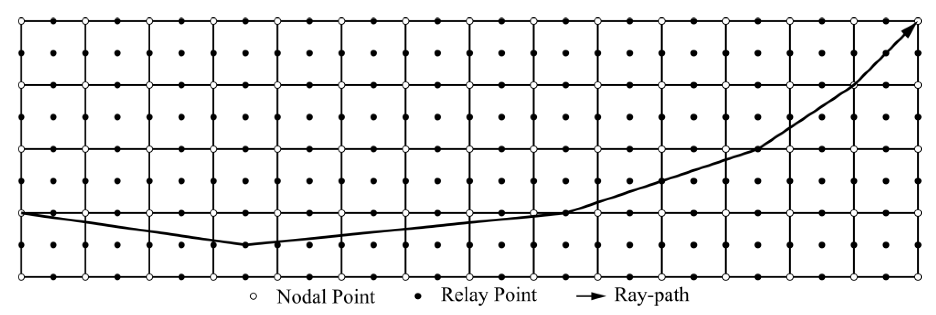
Conventionally, the source locations have been identified on the basis of a ray-trace technique on finite element meshes in AET. Figure 1 shows an example mesh on the area of interest, and an approximated ray-path. The area of interest is meshed by following the way of the finite element analyses, and the relay points are installed with a specified resolution in the source localization technique. The ray-paths are approximated as polylines, for which the apexes are located at nodal or relay points on the mesh. If it is assumed that elastic wave velocity is constant in individual cells, a travel time on an approximated ray-path is given as follows:

$$T_{ij}={\displaystyle \sum }_k{S}_k{\ell }_{ik}$$

(1)

where $T_{ij}$ is a travel time from point $i$ to point $j$; ${\ell }_{ik}$ is a length of a ray-path from point $i$ to point $j$ on cell $k$; and $S_k$ is a slowness, a reciprocal of elastic wave velocity, of cell $k$. Although this equation gives a travel time of any ray-paths between two points on the mesh, generally an important ray-path is the one that gives a first travel time. Thus, practically, the travel times of all of the ray-paths between the two points are computed using Equation (1), and then the ray-path that gives a minimum travel time is chosen as the ray-path that gives the first travel time on the ray-trace technique.

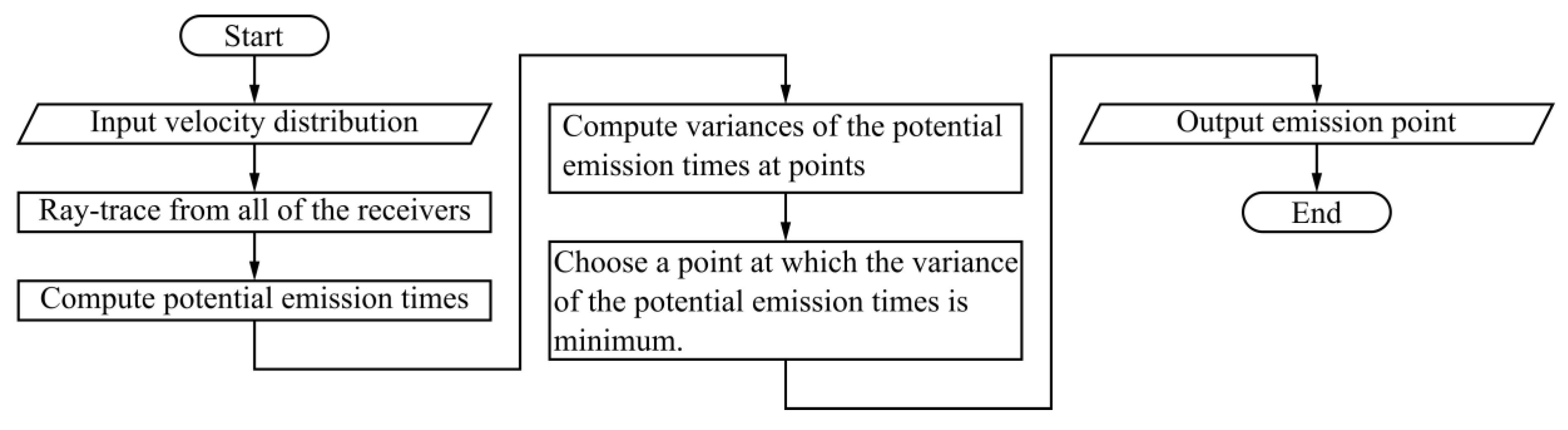
The conventional source localization technique is structured on the basis of the ray-trace technique. It is assumed that the locations of the receivers and the arrival times of the elastic waves that are emitted from a source location are known at the receivers on the source localization technique. A conceptual flow diagram of the conventional source localization technique is illustrated in Figure 2. Firstly, ray-trace is performed from all of the receivers to the nodal and relay points on the mesh, in order to compute the first travel times between them. Then, the potential emission times are computed on every nodal and relay points, as follows:

$$P_{ijk}=A_{ik}-T_{jk}$$

(2)

where $A_{ik}$ is the arrival time of event $i$ at point $k$, and $P_{ijk}$ is a potential emission time that is estimated for event $i$ on the basis of the arrival time $A_{ik}$ at point $j$. This potential emission time implies that an elastic wave of event $i$ must be emitted at $P_{ijk}$, if the elastic wave is emitted from point $j$ and arrives at point $k$, at $A_{ik}$. As a consequence, each nodal and relay point has $n$ potential emission times in a single event, if $n$ receivers are installed on the area of interest. It should be noted that the potential emission times should be identical at a point where the elastic wave is emitted, if the representations of the elastic wave velocity distribution and approximated ray-paths are identical to the real ones. However, generally, the point does not exist as the representations are normally insufficient. Therefore, a point where a variance of the potential emission times is minimum is chosen as the emission point in this technique.

The conventional source localization technique identifies the source location at a nodal or a relay point, and this immediately implies that the resolution of the identified source location is determined by the density of the nodal and the relay points. Figure 3 shows an example of an identified source location on a two-dimensional model. As illustrated in Figure 3, if a true source location exists in the center of a region that is surrounded by adjacent nodal and relay points, the source location is identified at a location of one of the nodal and relay points. Thus, the maximum error of the source location is half of the longest interval of two of the adjacent nodal and relay points. This fact reveals that the resolution of the source locations is half of the longest interval. This causes errors of a resultant elastic wave velocity distribution, because the arrival times of the elastic wave at the receivers are computed by using the identified source locations and the estimated emission times in AET.

The error of the resultant wave velocity distribution would be severe if the distance between a true source location and a receiver is close, as the error is relatively large in comparison with a length of a ray-path between the true source location and the receiver, and the dense installation of the relay points is required for reducing the errors. However, the computational costs of the ray-trace technique are proportional to the square of the total number of nodal and relay points, and the fine installation of the relay points drastically raises its computational costs. Hence, the fine installation of the relay points should be avoided from a practical point of view.

2.2. A New Source Localization Technique

The authors proposed an improved technique for raising the resolution, with a limited rise in the computational costs. This technique locally raises the resolution by installing extra source candidates in an area surrounded by the adjacent nodal and relay points of a roughly identified source location based on the conventional source localization technique [3]. Although this technique could reduce the computational costs on the same resolution in comparison with the conventional technique, the computational costs are still expensive if a fine resolution is required or the number of events is large, because the total number of the potential source candidates is also large.

A new source localization technique that has been developed on the basis of the previously introduced source localization technique is proposed in this study. The extra source candidates are installed in the area surrounded by the adjacent nodal or relay points of a roughly identified source location, with an interval that is half of the interval of the nodal and relay points, as illustrated in Figure 4, and a source location is identified by using the installed source candidates. Then, the extra source candidates are installed again in the vicinity of the identified source location. with an interval that is half of the previous interval, as illustrated in Figure 4, and the source locations are identified again using the newly installed source candidates. This procedure is iteratively performed until the desirable resolution is achieved, and finally, the source location is identified in the required resolution. This technique is characterized by the method of installation of the extra source candidates, and it is expected that the total number of the points is reduced by using this technique. The extra source candidates are sparsely installed in the compact box in the initial stage, and the resolution become twice in every iterative procedure, by moving the center of the compact box to the newly identified source location, and by changing the interval to half of the previous interval in this technique. This approach drastically reduces the total number of extra source candidates in comparison with the previous technique, in which the extra source candidates must be installed homogeneously with a target resolution in the vicinity of the roughly identified source location.

2.3. Numerical Example for Verifications of the Proposed Technique

The proposed technique is verified by performing a series of numerical investigations on a three-dimensional problem. Figure 5 shows a numerical model that is used for the verification. The model is a cube with an edge of 10 m, and the model is meshed with cubes with an edge of 1 m. Therefore, each edge is divided into 10 cells, and consequently, the total number of cells is 1000 in this model. Relay points are installed with an interval of 0.500 m. Hence, the maximum error of the source locations is 0.866 m in the conventional source localization technique. It is assumed that the receivers are installed at the apexes of the cube. Thus, the total number of receivers is eight. One hundred source locations are randomly generated in the model, and ray-trace is executed from the generated source locations to the receivers, so as to compute the arrival times of the elastic waves at the receivers. The source locations are identified on the basis of the presented source localization technique by using the computed arrival times as the observed arrival times, and its capability is verified by comparing the identified source locations and the generated source locations. The target resolution is changed to 25.0 cm, 12.5 cm, 6.25 cm, 3.13 cm, and 1.56 cm in this verification.

3. Results

Figure 6a,b shows the results of the source localization in the interval of 25.0 cm and 1.56 cm, respectively. According to Figure 6, it is confirmed that the proposed technique identifies the source locations adequately, and the accuracy of the source localization is raised by raising the resolution. The distances of the black spheres and white spheres show the errors of the identified source locations, and these errors are larger in the case of an interval of 25.0 cm, in comparison with the case of an interval of 1.56 cm, according to Figure 6. Figure 7 shows the average distances between the true source locations and the identified source locations. According to Figure 7, the average distances decrease with the raising of the resolution. These results reveal that the accuracies of the identified source locations are raised in the fine resolution.

4. Discussion

This implementation aims to achieve a high resolution with a reduced number of source candidates compared with the previously introduced source localization technique. The cost of the source location techniques depends on the cost of the ray-trace technique, and the cost of the ray-trace technique is mainly determined by the number of total points. Hence, the computational costs are reduced if the total number of points is reduced. The total number of nodal and relay points is 9261 in this model, as the nodal points are installed with an interval of 1.0 m, and the relay points are installed with an interval of 0.50 m. The total number of the extra source candidates is 135 per event, as 27 extra source candidates are installed for respective resolution in this case. Thus, the total number of the points is 22,761. However, approximately 253 million points are necessary in order to achieve the same resolution as the conventional source localization technique, and it is impossible to do the computation with a typical computer. This difference entails a drastic change of computational costs and would allow the application of this technique for practical projects.

5. Conclusions

The new source localization technique was introduced and its capability was verified by performing a series of the numerical investigations. The conclusions of this study are drawn below.

• The new source localization technique adequately identifies source locations on heterogeneous elastic wave velocity distribution, based on the ray-trace technique.
• The accuracy of the source locations is determined by the interval of the extra source candidates that is immediately correlated with the resolutions of the source localization.
• The total number of the source candidates is smaller in the introduced source localization technique compared with the conventional source localization technique.

References

1. Kundu, T. Acoustic source localization. Ultrasonics 2014, 54, 25–38. [Google Scholar] [CrossRef] [PubMed]
2. Kobayashi, Y.; Shiotani, T. Computerized AE Tomography, Innovative AE and NDT Techniques for On-Site Measurement of Concrete and Masonry Structures State-of-the-Art Report of the RILEM Technical Committee 239-MCM; Springer: Berlin, German, 2016; pp. 47–68. [Google Scholar]
3. Kobayashi, Y.; Oda, K.; Tamura, Y.; Fuse, T.; Shiotani, T. Source location algorithm with controlled resolution based on ray-trace technique. In Proceedings of the Second International RILEM/CONST Conference on Early Age Cracking and Serviceability in Cement-Based Materials and Structures, Brussels, Belgium, 12–14 September 2017; pp. 161–166. [Google Scholar]
Figure 1. An approximated ray-path on a finite element mesh with relay points.
Proceedings 02 00477 g001
Figure 2. Conceptual flow diagram of the conventional source localization technique based on the ray-trace technique.
Proceedings 02 00477 g002
Figure 3. An example of an identified source location on a two-dimensional model.
Proceedings 02 00477 g003
Figure 4. A new source localization technique.
Proceedings 02 00477 g004
Figure 5. A numerical model for the verifications.
Proceedings 02 00477 g005
Figure 6. Results of the source localization (black spheres: identified source locations; white spheres: true source locations).
Proceedings 02 00477 g006
Figure 7. Interval of extra source candidate vs. average error of identified source locations.
Proceedings 02 00477 g007
Publisher’s Note: MDPI stays neutral with regard to jurisdictional claims in published maps and institutional affiliations.