A Robust Test-Based Modal Model Identification Method for Challenging Industrial Cases ^†

Abstract

In this paper, the MLMM modal parameter estimation method (Maximum Likelihood estimation of a Modal Model) and its new variant will be introduced. The MLMM method tackles some of the remaining challenges in modal analysis (e.g., modal analysis of highly-damped cases where a large amount of excitation locations is needed such as the modal analysis of a trimmed car body). Another big advantage of the MLMM method is its capability to fully integrate, within the estimated modal model, some important physical constraints, which are required for the intended applications, e.g., realness of the mode shape and FRFs reciprocity. More classical modal parameter estimation methods have rarely the possibility to fully integrate these constraints and the obtained modal parameters are typically altered in a subsequent step to satisfy the desired constraints. It is obvious that this may lead to sub-optimal results. The MLMM method uses the Levenberg-Marquardt optimization scheme to directly fit the modal model to the measured FRFs. The applicability of MLMM to estimate an accurate constrained modal model will be demonstrated using two challenging industrial applications.

1. Introduction

The modal model expresses the dynamic behavior of a linear time-invariant system as a linear superposition of the contributions from different vibration modes of the structure where each vibration mode is expressed in terms of its modal parameters: resonance frequency, damping ratio, mode shapes, and participation factors. To determine those modal parameters, the starting point is usually a set of measured frequency response functions (FRFs). The relation between the modal parameters and the measured FRFs $H\left({\omega }_k\right){ℂ}^{N_o\times N_i}$ ($N_o$ the number of outputs, $N_i$ the number of inputs) is expressed in Equation (1).

$$H\left({\omega }_k\right)=\left({\displaystyle \sum }_{r=1}^{N_m}\left(\frac{{\psi }_r{L}_r}{s_k-{\lambda }_r}+\frac{{\psi }_r^{*}{L}_r^{*}}{s_k-{\lambda }_r^{*}}\right)\right)+\frac{LR}{s_k^2}+UR$$

(1)

with $N_m$ the number of identified modes, ${\psi }_r\in {ℂ}^{N_o\times 1}$ the rth mode shape, ${\lambda }_r$ the rth pole, $s_k=j{\omega }_k\left(k=1,2,\dots ,N_f\right)$,$N_f$ the number of frequency lines, ${()}^{*}$ stands for the complex conjugate of a complex-valued parameter, $L_r\in {ℂ}^{1\times N_i}$ the rth participation factors, $LR\in {ℝ}^{N_o\times N_i}$ and $UR\in {ℝ}^{N_o\times N_i}$ the lower and upper residual terms. The lower and upper residual terms are modeling the influence of the out-of-band modes in the considered frequency band. The fundamental problem of modal parameter estimation consists of adjusting the modal parameters in the modal model, so that the data predicted by the model approximates the measured data as closely as possible. Once the modal model (1) is estimated and validated it can serve as a base for a redesign process for optimizing the system dynamic behavior. Two important applications of the experimentally driven modal models are the structural static stiffness identification and the NVH refinement of a fully trimmed car body. Estimating reliable modal models for those two applications requires: (1) the use of many excitation locations to sufficiently excite the modes of the car body due to the high level of damping and high modal density; and (2) the identified modal model must fulfill some physical constraints, e.g., FRFs reciprocity and the realness of the mode shapes. The more classical modal parameter estimation methods fail to achieve a high-quality curve-fit of an FRF matrix with large number of columns (e.g., >4). Moreover, classical modal parameter estimation methods have rarely the possibility to fully integrate some physical constraints (e.g., FRFs reciprocity) and the obtained modal parameters are typically altered in a subsequent step to satisfy the desired constraints. It is obvious that this may lead to sub-optimal results, as for instance evidenced by a degradation of the quality of the fit between the identified modal model and the measurements. Hence, a non-reliable modal model is estimated, and consequentially erroneous results are obtained.

In this paper, a recently-developed modal parameter estimation method called MLMM (Maximum Likelihood estimation of a Modal Model) and its new feature will be presented. The MLMM uses the well-established statistical concept of maximum likelihood estimation to estimate directly a modal model based on measured FRFs. In MLMM, the parameters of the modal model (1) are optimized using the Levenberg-Marquardt optimization scheme. Desired physical constraints (e.g., FRFs reciprocity, realness of mode shapes, etc.) can be applied on the identified modal model and directly considered in the optimization process, which significantly reduces the impact of these constraints on the quality of the final estimated modal model. By means of two challenging industrial applications, the capability of the MLMM to deliver accurate modal models will be demonstrated.

2. MLMM Modal Parameter Estimation Method

2.1. MLMM: Basic Background

The MLMM modal parameter estimation method is a multivariable (i.e., MIMO) frequency-domain method that uses the modal model as a parametric model to represent the measured FRFs over a chosen frequency band. The MLMM method is originally introduced in [1] and further improved in terms of the computational load in [2]. In [3], the MLMM method is adapted to consider some desired physically motivated constraints (e.g., FRFs reciprocity) in the optimization process. The MLMM method differs from the existing modal parameter estimation methods in the sense that it directly optimizes the modal model, represented by Equation (1), rather than optimizing a high order rational fraction polynomial-based model and reducing it in a subsequent step to a modal model that leads at the end to sub-optimal results. The optimization process tunes the parameters of the modal model to minimize the following quadratic-like cost function so that a best match between the modal model and the measurements is obtained:

$${\ell }_{MLMM}\left(\theta \right)={\displaystyle \sum }_{i=1}^{N_i}{\displaystyle \sum }_{o=1}^{N_o}{\displaystyle \sum }_{k=1}^{N_f}{\left|E_{io}\left(\theta ,{\omega }_k\right)\right|}^2,\mathrm{where}{E}_{io}\left(\theta ,{\omega }_k\right)=\frac{H_{io}\left({\omega }_k\right)-{\widehat{H}}_{io}\left(\theta ,{\omega }_k\right)}{{\sigma }_{H_{io}}\left({\omega }_k\right)}$$

(2)

with $E_{io}\left(\theta ,{\omega }_k\right)\in ℂ$ the weighted residual (i.e., the error between the measured FRF $H_{io}\left({\omega }_k\right)$ and the estimated FRF ${\widehat{H}}_{io}\left(\theta ,{\omega }_k\right)$ represented by the modal model in Equation (1)) and ${\sigma }_{H_{io}}\left({\omega }_k\right)$ the standard deviation of the measured FRF for output $o$ and input $i$. This residual $E_{io}\left(\theta ,{\omega }_k\right)$ is a nonlinear function of the modal model parameters $\theta$. In case the noise information (i.e., ${\sigma }_{H_{io}}\left({\omega }_k\right)$) is not available, the method can still be used with unweighted error equation. The optimized estimates of $\theta$ (i.e., ${\psi }_r$,$L_r$,${\lambda }_r$,$LR$, and $UR$) will be obtained by minimizing the cost function ${\ell }_{MLMM}\left(\theta \right)$ using the Levenberg-Marquardt optimization algorithm. To start this non-linear optimization problem, initial values for all the modal parameters are estimated by the well-known LMS Polymax method [4,5]. The Jacobian matrix that is needed for the optimization process is calculated analytically by driving the derivatives of the error equation with respect to all the parameters of the modal model (1) (i.e., $\partial E/\partial \theta$).

Constraints on the identified modal model can be imposed by the user before staring the estimation process. If the objective is to validate a proportionally damped finite element model (FEM), the MLMM can be limited to finding the best fit modal model with purely imaginary residue matrices meaning that $\Re \left({\psi }_r{L}_r\right)=0$ in Equation (1) which is mathematically consistent with the numerical models. Similarly, reciprocity of the modal model can be imposed upfront, avoiding the risk of degrading the model quality by imposing the reciprocity requirement after the estimation. Imposing reciprocity in the modal model (1) implies that the residue matrices ${\psi }_r{L}_r$ and the residual matrices $LR$ and $UR$ are imposed to be symmetric.

2.2. MLMM: A New Feature

According to the modal theory, a physical vibration mode should yield a negative mass sensitivity [6] meaning that adding a mass to a mechanical structure at a measurement point will decrease the damped natural frequencies for all modes. This is a very important property of the modal model especially when correlating a FE model with an experimentally driven modal model. If the mode is estimated with a positive mass sensitivity (PMS), it could be that this mode is related to a dubious pole (e.g., computational pole that models noise effects), or it is poorly excited mode. In both cases, this mode should be removed from the mode set before using it for the intended application. A new feature that enables the automatic rejection of such modes (i.e., the ones estimated with PMS) from the mode set during the optimization process is added to the MLMM method.

3. Applications

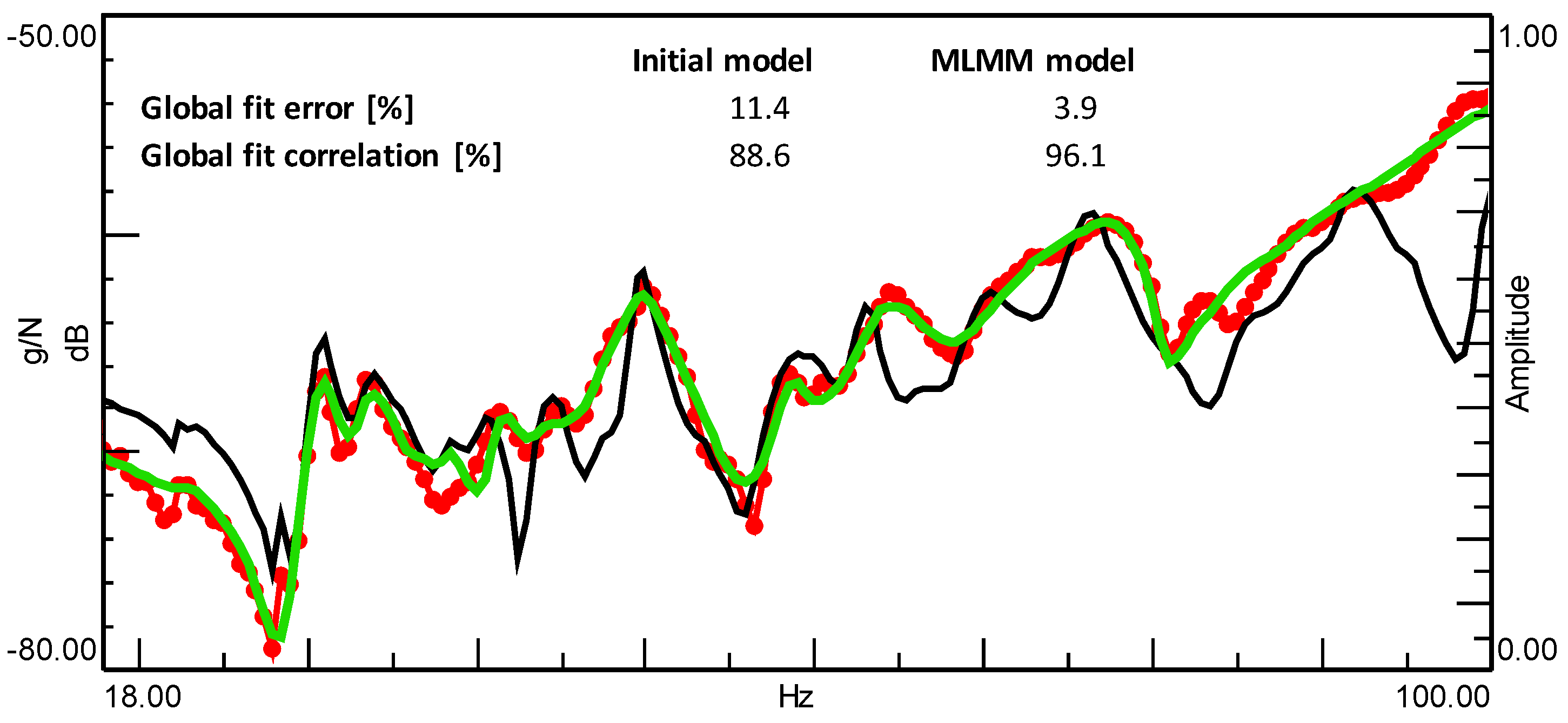
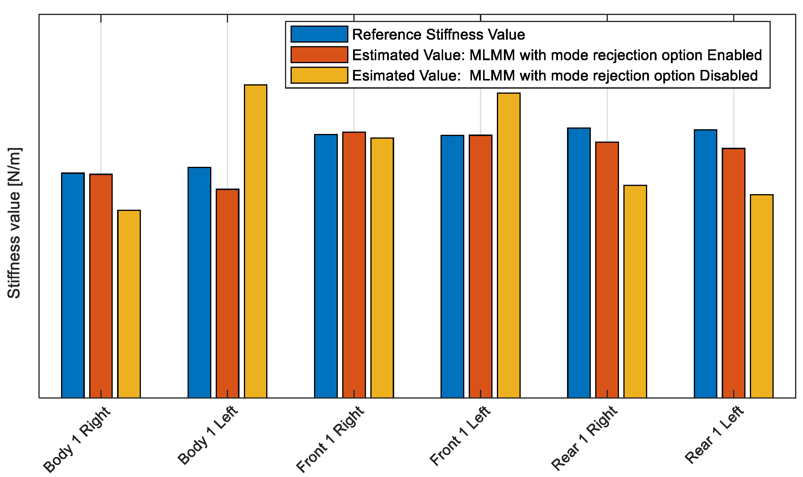
3.1. Application of MLMM Method to Trimmed Car Body Structural Data Set

A modal test is done in free-free condition on a trimmed car body where the car body is excited at 40 locations and the resulting acceleration responses are measured in 3 degrees of freedom at series of output points (40+) distributed over the car body. This modal test aims to obtain an experimentally driven modal model that can be used to identify the structural static stiffness at some connection points at the structure of the car body. The static stiffness is defined by both the global body characteristics as global torsional, bending, and shear modes (i.e., modes <100 Hz) as well as local body characteristics (i.e., modes >100 Hz). The modal model of the trimmed body has been identified through the combined use of LMS Polymax and MLMM estimators, representing the global dynamics up to 100 Hz. An initial modal model is generated by applying the Polymax estimator to the measured FRFs. Afterwards, MLMM method is used to further optimize the initial modal model considering that the model verifies the reciprocity and the mode shapes realness constraints. The new option added to the MLMM estimator that enables the automatic rejection of the modes that have a PMS during the iterations is enabled. For this analysis, a limited number of references (e.g., 6 columns of the FRFs matrix) are used for the estimation process. The initial mode set generated by the Polymax estimator has 69 modes, and the MLMM retains 54 modes at the end of the iterations. This means that 15 modes are rejected by MLMM during the optimization because they are estimated with a PMS.

The comparison between the modal model identified by the MLMM and the initial one is presented in Figure 1 by comparing one of the synthesized FRFs to the measured one. Clear advantage of MLMM usage is demonstrated in Figure 1 where the obtained modal model closely fits the measured FRF in comparison with the initial modal model. By using the identified modal model that represents this dynamic data the static stiffness can be identified by excluding the rigid body and the out-of-band behavior from the modal model. The stiffness value estimated for some points using the identified MLMM modal model is shown and compared to the expected (reference) values in Figure 2. In this figure, the impact of the new option added to the MLMM estimator, which enables the rejection of the modes that have a PMS, on the reliability of the results is demonstrated. A trimmed body (TB) modal model is built based on MLMM enabling the PMS modes rejection option and a second TB modal model is built using MLMM while disabling that option. The reference value shown in Figure 2 is estimated based on modal model that has been built by fitting an FRFs matrix that has 40 columns (i.e., 40 excitation locations) using MLMM. Results in Figure 2 are shown for point pairs, i.e., each point exists on the both sides of the car.

From this figure, it can be concluded that even by using a limited number of references (i.e., 6 inputs) the MLMM method with the new added option (i.e., automatic rejection of modes with PMS) is capable to deliver a more reliable modal model that gives more realistic estimates for the static stiffness in terms of the magnitude and the distribution over the car body. The MLMM with the mode rejection option enabled gives stiffness values that are closer to the expected value and that are symmetric as would be expected on a typical car body structure.

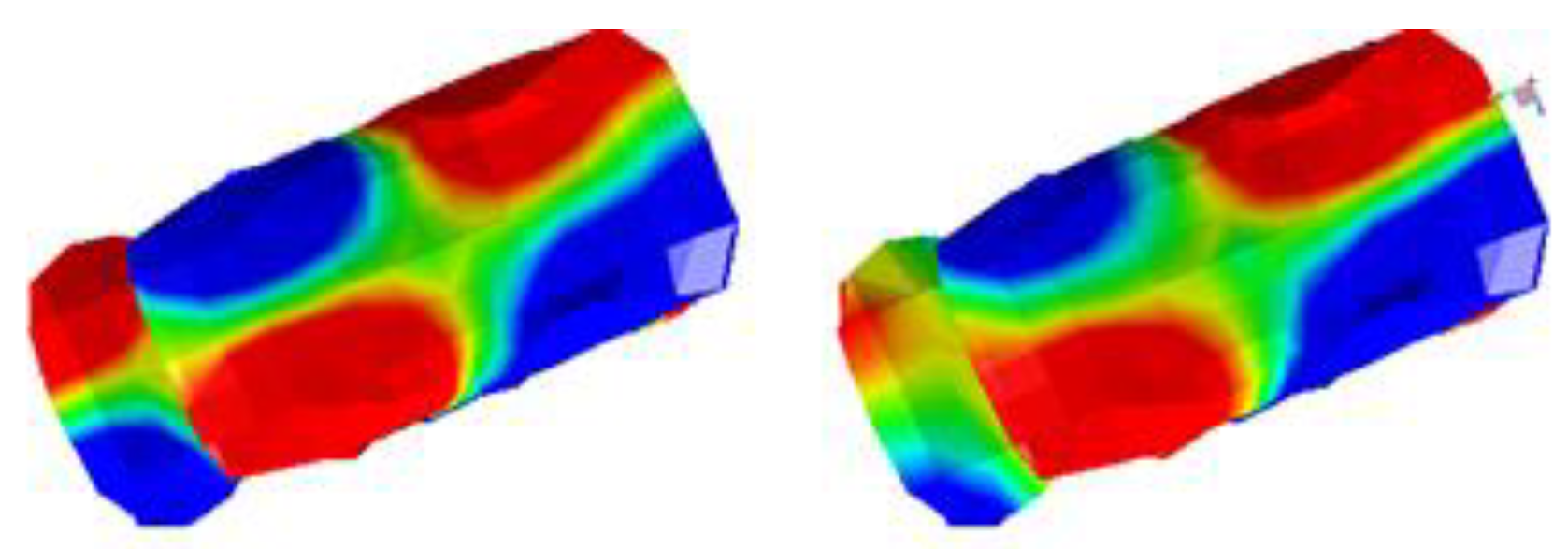
3.2. Application of the MLMM Method in the Field of Acoustic Modal Analysis (AMA) of a Car Cavity

In this application, many excitation locations were also needed as in the previous example as well to get sufficient excitation of the acoustic modes across the entire cavity of the car and to avoid mode shape distortion that typically occurs when low number of acoustic sources are used [9]. Multiple inputs multiple outputs (MIMO) acoustic modal analysis test was carried out inside the cavity of a car where the car cavity is acoustically excited at 12 locations using loudspeakers and the sound pressure is measured at 612 locations using microphones. Detailed description of the measurement can be found in [7]. The FRFs matrix used for the modal parameter estimation consists of 527 rows, 10 columns, and 450 spectral lines. It has been observed that the classical modal parameter estimation methods have some difficulties in fitting an FRFs matrix with such number of columns (i.e., inputs) [8,9]. The LMS Polymax estimator was applied to that large database in the frequency band of 44 till 220 Hz. Based on the Polymax stabilization chart, 13 modes were retained. The acoustic cavity and the flexible walls of the cavity constitute a coupled vibro-acoustic system and hence the modes of the system generally will consist of an acoustic part (pressure waves in cavity air) and a structural part (flexural waves in cavity walls). Therefore, and even though both excitation and measured response quantities are from the acoustic domain, also more structural related modes may be retrieved from the analysis. Nevertheless, it appears that the selected modes are to a large extent “acoustically dominant” modes. Using the same Polymax poles, both real and complex mode shapes have been estimated. The curve-fitting quality is represented in

Table 1. Mean fitting error & correlation between the measured and synthesized FRFs: real and a complex mode shapes-based modal model is fitted.

	Polymax		MLMM
Mean Value	Real	Complex	Real	Complex
Fitting Error [%]	27.7	20.9	9.6	5.6
Fitting Correlation [%]	79.3	84.6	92.1	95.2

(Polymax columns). Afterwards, 10 MLMM iterations are applied to the Polymax initial estimates, both using the general complex mode formulation of the modal model and the constrained real-mode shapes modal model. Also, the MLMM results are represented in Table 1. Whereas Table 1 provides averaged results over all FRFs, Figure 3 shows the curve-fitting results of a typical FRF. From Table 1 it can be concluded that, obviously, the fitting quality degrades when using real instead of complex mode shapes in Polymax (i.e., initial generated modal model).

When comparing MLMM with Polymax, substantial improvements are obtained in terms of curve-fitting quality, both for general complex modes and real modes. Interesting to observe is that the real mode shapes MLMM-based results are superior to the complex mode shapes Polymax-based results, indicating that although the real mode shapes-based modal model has less parameters that can be tuned, still superior results are obtained, thanks to the optimization process in MLMM. An example of a real and complex mode shape pair is provided in Figure 4. The (complex) mode shape (Right) had quite high complexity indicators: MPC = 84%, MPD = 26°. Real mode shapes are typically easier to interpret and may be more suited for correlation with FE models [10].

4. Conclusions

The MLMM modal parameter estimation method is introduced and validated using two challenging real-life applications that are of great interest to the automotive OEMs. The MLMM method estimates directly the modal model starting from a set of measured FRFs using Levenberg-Marquardt optimization scheme, and it has the advantage that it can integrate physical constraints (e.g., FRFs reciprocity and realness of the mode shapes) in the identified modal model directly during the optimization process. A new feature is added to the MLMM method which enables the user to automatically reject modes that have positive mass sensitivity during the optimization process. From the obtained results it can be concluded that by combining the features of both Polymax and MLMM estimators more reliable constrained modal models that are able to accurately represent the measured FRFs can be identified and used for the intended application.

References

1. El-Kafafy, M.; De Troyer, T.; Peeters, B.; Guillaume, P. Fast Maximum-Likelihood Identification of Modal Parameters with Uncertainty Intervals: A Modal Model-Based Formulation. Mech. Syst. Signal Process. 2013, 37, 422–439. [Google Scholar] [CrossRef]
2. El-kafafy, M.; Accardo, G.; Peeters, B.; Janssens, K.; De Troyer, T.; Guillaume, P. A Fast Maximum Likelihood-Based Estimation of a Modal Model. In Topics in Modal Analysis; Mains, M., Ed.; Springer International Publishing: Berlin/Heidelberg, Germany, 2015; Volume 10, pp. 133–156. [Google Scholar]
3. El-Kafafy, M.; Peeters, B.; Guillaume, P.; De Troyer, T. Constrained Maximum Likelihood Modal Parameter Identification Applied to Structural Dynamics. Mech. Syst. Signal Process. 2016, 72–73, 567–589. [Google Scholar] [CrossRef]
4. Guillaume, P.; Verboven, P.; Vanlanduit, S. Van der Auweraer, H. In Peeters, B. A poly-reference implementation of the least-squares complex frequency domain-estimator. In Proceedings of the 21th International Modal Analysis Conference (IMAC), Kissimmee, FL, USA, 3–6 February 2003. [Google Scholar]
5. Siemens PLM (LMS International). LMS Test.Lab. Available online: www.plm.automation.siemens.com (accessed on 1 March 2018).
6. Heylen, W.; Lammens, S.; Sas, P. Modal Analysis Theory and Testing; Katholieke Universiteit Leuven: Heverlee, Belgium, 1997. [Google Scholar]
7. Accardo, G.; El-kafafy, M.; Peeters, B.; Bianciardi, F.; Brandolisio, D.; Janssens, K.; Martarelli, M. Experimental Acoustic Modal Analysis of an Automotive Cabin. In Experimental Techniques, Rotating Machinery, and Acoustics; de Clerck, J., Ed.; Springer International Publishing: Berlin/Heidelberg, Germany, 2015; Volume 8, pp. 33–58. [Google Scholar]
8. Peeters, B.; El-Kafafy, M.; Accardo, G.; Knechten, T.; Janssens, K.; Lau, J.; Gielen, L. Automotive cabin characterization by acoustic modal analysis. In Proceedings of the JSAE Annual Congress, Sendai, Japan, 22–24 October 2014. [Google Scholar]
9. Yoshimura, T.; Saito, M.; Maruyama, S.; Iba, S. Modal analysis of automotive cabin by multiple acoustic excitation. In Proceedings of the ISMA2012-USD2012, Leuven, Belgium, 17–19 September 2012. [Google Scholar]
10. Hwang, K.H.; Choi, S.C.; Van Genechten, B.; Jeon, J.H.; Brechlin, E. Acoustic finite element model validation of vehicle interior cabin from acoustic mode and transfer function. In Proceedings of the NAFEMS World Congress, San Diego, CA, USA, 21–24 June 2015. [Google Scholar]
Figure 1. An example of the synthesized fit together with the mean (over all the FRFs) fit error and correlation: Red: Measured Black: synthesized initial model Green: MLMM optimized model.
Proceedings 02 00378 g001
Figure 2. Static stiffness for some selected points in lateral direction using modes <100 Hz (For confidentiality reasons the stiffness values cannot be shown).
Proceedings 02 00378 g002
Figure 3. Figure 3. Typical acoustic FRF curve-fitting results. MLMM with real modes performs better than the traditional (real and complex) approach Polymax cases.
Proceedings 02 00378 g003
Figure 4. (Left) Easily interpretable Real mode shape; (Right) complex mode shape with phase differences.
Proceedings 02 00378 g004