Abstract
Clouds and cloud-shadow are a persistent problem in all optical satellite imagery. Plenty of methods have been suggested in the literature to address this problem, and reconstruct the missing part of the optical signal. In this work, three methods representative of different approaches to the cloud removal problem were compared. The first method is temporal fitting using Fourier series, which benefits from the temporal continuity of the signal. The second method uses sparse spectral unmixing to fill in the missing areas. The third method employs radiometric consistency as a tool to determine the missing part of the signal. These three methods were first presented and their theoretical background described, followed by a discussion of their implied assumptions and general performance. A set of experiments using Landsat 8 time series with diverse land cover types were conducted. The quantitative results of the three methods using simulated clouds are presented. Finally, some concluding remarks about the relative advantages of the three approaches are listed, in addition to some recommendations about their use.
1. Introduction
For any optical space-borne imaging sensor, the atmosphere represents an unavoidable noise source. Around 70% of the earth surface is covered by clouds in any single moment [1], which makes the phenomenon of cloud and cloud-shadow a persistent one. It is possible to minimize the effect of clouds and other similar atmospheric degradation by employing a signal recovery method. There are three main directions researchers often follow to implement such a method. The first category of algorithms which is robust in theory but often difficult to implement is sensor fusion, which has strict requirements, such as matching temporal and spatial resolution, making it unrealizable in many cases. Knauer et al. [2] fused MODIS data with Landsat 8 to generate high temporal frequency, high spatial resolution, cloud-free time series. The algorithm uses linear regression to estimate the value of each pixel at Landsat resolution, by using two time series, one for MODIS and the other for Landsat. By fusing three different types of data, namely low resolution optical image and a SAR image, along with the target high resolution multispectral data, Li et al. [3] recovered the missing part in the latter. The algorithm uses dictionary group learning to relate the three data sources together. The coefficients used to recover the cloudy patches are found using non-local joint sparse coding. A second class of methods, which is only sporadically investigated, is to reconstruct the missing part of an image using the clear part, a technique known as inpainting. Inpainting family of methods uses the cloud free part of the image to reconstruct the contaminated part. Maalouf et al. [4] used the continuity of geometric flow of the image to synthesize the geometry inside the cloudy part. Bandlet transform followed by multiscale grouping was employed to learn the geometrical structure of the clear portion of the image. In [5], Cheng et al. proposed an inpainting algorithm based on a multichannel nonlocal variational model. A nonlocal operator is formulated within a variational framework, and then an iterative optimization algorithm is used to find the weights for this operator. The third direction in dealing with the cloud problem has been given much more attention, that of using a time series to interchangeably recover the missing parts in all individual scenes. The idea here is to use the temporal correlation of the signal to predict the missing part. The underlying assumption is that the signal is continuous in time.
Xu et al. [6] suggested a method based on sparse reconstruction. The algorithm learns multitemporal dictionary using the cloud-free parts of the images. Instead of random dictionaries as in the case of [7], the dictionary for the cloudy image is calculated using iterative optimization method. Cheng et al. [8] presented an algorithm that fills the cloud contaminated areas pixel by pixel. A matching pixel is found using a spatio-temporal Markov Random Field (MRF). A cloud-free reference image is used in the optimization of MRF energy terms. The method is applicable to different sensors (MODIS, Landsat, etc.).
A good review for many of the recent work about image reconstruction in satellite images recovery was presented by Shen et al. [9]. The different algorithms have been categorized according to the data relationship they exploit. This led to four different types of algorithms, i.e. spatial methods, spectral methods, temporal methods and hybrid methods, which combine more than one approach.
To the best of our knowledge, there is no comprehensive comparison of the different methods suggested for the problem of cloud removal. Therefore, it is extremely difficult to decide which method to use for what kind of data or what type of task. This work investigated three methods for the challenging problem of cloud recovery; these methods were compared from a theoretical perspective as well as empirically. The relative advantages expected from theory were tested using diverse data sets, representing urban, crops and bare-land.
2. Method
A brief overview of the three compared algorithms is presented below.
2.1. Temporal Fitting Using Fourier Series
Brooks et al. [10] approached the problem of cloud removal as a regression problem in the time domain. The scenes are stacked together to form a time series, with missing parts in some of the scenes or all of them. The algorithm assumes a cyclic temporal signal, the full cycle length is typically an integer number of years.
The algorithm performs harmonics fitting at a pixel level using Fourier series. For each corrupted pixel, a vector of length N is constructed, where N is the cycle length. For a year cycle, , where each month is represented by one scene. For a pixel p, which has a spectral vector , for a time series of length d. If the pixel is cloudy, and falls within a temporal gap exceeding a fixed threshold g, then the algorithm fills it as follows:
- Interpolate p to produce the full length time series , with length N. The interpolated points are only there to get a better estimate of the harmonics parameters
- Use least square estimation to estimate the coefficients
- Discard the filled point, then use the found coefficients a to estimate the point
In this work, the standard one-year cycle was used, with . The gap was set to 1 to achieve one scene per month. The apparent advantage of Fourier fitting is its ability to tackle any time series, regular or not. It can also be adapted to multi-year long time series.
2.2. Unmixing
Sparse Unmixing-Based Denoising (SUBD) is used typically in hyperspectral data to restore bands which are affected by low signal-to-noise ratio. If multispectral data are stacked in a form of a time series, it is possible to use the same principle in the problem of cloud removal, provided that enough scenes are available. For Landsat data, with 6 usable bands, it is possible to use SUBD with as few as 5 scenes.
The main principle of the method is to recover a missing pixel as a linear combination of endmembers, with linear weights.
where is the reconstructed pixel, are the endmembers, k is the number of endmembers, and the corresponding weights. Cerra et al. [7] applied SUBD to recover the cloudy parts of multispectral time series.
To implement this method, LARS solver was used, with 100 randomly selected endmembers as in the original paper. The unmixing method can recover the missing parts with good quality, as long as enough data to select the endmembers is available.
2.3. Information Cloning
The information cloning method developed by Lin et al. [11] addresses the cloud recovery as a global optimization problem. It utilizes a temporal correlation of multitemporal images, and clones patches from cloud-free images which match well with radiometric conditions of the reference image. The algorithm solves Poisson equation using Dirichlet boundary conditions
where f is an unknown function responsible for generating the image and V is a guidance vector.
- Calculate the image quality factor for each scenewhere is mean of image I, is the reference image, is the target image, is the covariance coefficient between images and , and are constants. Only the cloud-free pixels are used in the computation of
- Sort the values for all images in an ascending order ( being the best match, and the worst).
- Extract the patches from the best images.
- Calculate the percentage of clouds in similar patches, discard any patch with cloud coverage higher than a specified threshold (set to 80%).
- Calculate the guidance vector V for each of the reference images (consider the images selected in the step above)where p is the target pixel and q is one of its neighbors (4th neighborhood used)
- Use the relaxation iterative method to solve the equation.
The information cloning method guarantees radiometric consistency, which means the reconstructed parts will tend to have a natural look.
3. Results
To evaluate the relative performance of the three different algorithms, an artificial cloud-mask was used. The mask was taken from an actual mask of a cloudy scene, where 11% of the scene is covered by clouds and shadow. Starting from a nearly cloud-free time series, the effect of the clouds and cloud-shadow was simulated using a cloud-mask with rather realistic clouds and shadows. Figure 1 depicts the output of the different algorithms in reconstructing the cloudy part of the image. The shadows are always treated like clouds in all used algorithms.
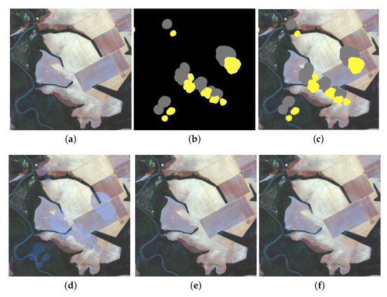
Figure 1.
Applying the three different algorithms on a crop scene. The cloud cover is 11% of the scene: (a) is the original scene; (b) the cloud mask; (c) the overlaid mask on top of the scene; (d) the output of the Fourier method; (e) Unmixing method; (f) Cloning method
Different land cover types were tested. The scenes used were covered by three different cover types, crops, urban and bare soil. As can be seen, all methods work quite well for this land cover type (crops). Fourier has some radiometric discontinuity at the borders, which is to be expected especially if rapid changes happen in between the scenes. Unmixing and cloning achieve good results.
Table 1 and Table 2 are computed for a time series of 10 scenes, with the target scene, which is the scene with the simulated clouds, in the fourth position. As can be seen in the table, all methods work considerably well with bare soil scene, with the lowest Mean Square Error (MSE), Mean Average Error (MAE), and consistently. The scene is very homogeneous with no challenge in recovering any part of it. This can also be confirmed by the visual metrics found in Table 2. This table lists SSIM measure Equation (6), and the Peak Signal to Noise Ratio (PSNR), computed as
where L is the maximum radiometric value possible for the data.

Table 1.
Error measures for the three approaches applied to different land covers.
Table 2.
Visual appeal indicators of all methods on various land covers.
SSIM and PSNR are structural and visual measures rather than error measures. For both measures, larger numbers indicate higher visual appeal of the image. For the algorithm performance, it is evident that the Unmixing algorithm is the best performer, achieving the lowest error in Table 1 and the best visual appeal in Table 2. The errors and visual appearance of the other two algorithms is not consistent across land cover types.
3.1. Failure Modes
There are various assumptions behind each of these methods, which lead to degradation of the accuracy once any of them is not fulfilled. The most notable assumption is the temporal correlation between the images, which is valid for all of the algorithms. If some rapid changes occur in the corrupt part of any scene, all methods will fail to recover a good estimate of the new land cover; they would rather use the temporal history to recover a temporally or radiometrically consistent scene. In addition, the following points apply to individual methods.
- Fourier fitting requires small gaps between the scenes; if the distribution of scenes along the time line is very irregular, it will work rather well for the dense part of the timeline, but resorts to simple linear interpolation in the sparse part of the line.
- Unmixing needs enough representation of each land cover in the visible part of the scene. As the dictionary is built by random sampling, the land cover types with very few cloud-free pixels will be difficult to include in the dictionary, therefore difficult to recover.
- Information cloning requires continuity in both temporal and radiometric spaces. If abrupt changes occur at the cloud boundary, recovering the scene will be very difficult, as the Poisson equation is solved using the boundary conditions.
4. Conclusions
The cloud removal problem is still an active area of research; by comparing different algorithms, it is possible to give some guidelines about which algorithm to use in which case. From the results of the experiments, it is possible to conclude that the Unmixing algorithm performs well, but this is rather difficult to generalize beyond the scope of these experiments. With different conditions, namely, dictionary size, cloud size and time series length, the performance of the Unmixing method will change drastically.
References
- Stubenrauch, C.; Rossow, W.; Kinne, S.; Ackerman, S.; Cesana, G.; Chepfer, H.; Di Girolamo, L.; Getzewich, B.; Guignard, A.; Heidinger, A.; et al. Assessment of global cloud datasets from satellites: Project and database initiated by the GEWEX radiation panel. Bull. Am. Meteorol. Soc. 2013, 94, 1031–1049. [Google Scholar] [CrossRef]
- Knauer, K.; Gessner, U.; Fensholt, R.; Kuenzer, C. An ESTARFM Fusion Framework for the Generation of Large-Scale Time Series in Cloud-Prone and Heterogeneous Landscapes. Remote Sens. 2016, 8, 425. [Google Scholar] [CrossRef]
- Li, Y.; Li, W.; Shen, C. Removal of Optically Thick Clouds from High-Resolution Satellite Imagery Using Dictionary Group Learning and Interdictionary Nonlocal Joint Sparse Coding. IEEE J. Sel. Top. Appl. Earth Obs. Remote Sens. 2017, 10, 1870–1882. [Google Scholar] [CrossRef]
- Maalouf, A.; Carre, P.; Augereau, B.; Fernandez-Maloigne, C. A Bandelet-Based Inpainting Technique for Clouds Removal from Remotely Sensed Images. IEEE Trans. Geosci. Remote Sens. 2009, 47, 2363–2371. [Google Scholar] [CrossRef]
- Cheng, Q.; Shen, H.; Zhang, L.; Li, P. Inpainting for Remotely Sensed Images with a Multichannel Nonlocal Total Variation Model. IEEE Trans. Geosci. Remote Sens. 2014, 52, 175–187. [Google Scholar] [CrossRef]
- Xu, M.; Jia, X.; Pickering, M.; Plaza, A.J. Cloud Removal Based on Sparse Representation via Multitemporal Dictionary Learning. IEEE Trans. Geosci. Remote Sens. 2016, 54, 2998–3006. [Google Scholar] [CrossRef]
- Cerra, D.; Bieniarz, J.; Beyer, F.; Tian, J.; Muller, R.; Jarmer, T.; Reinartz, P. Cloud Removal in Image Time Series Through Sparse Reconstruction from Random Measurements. IEEE J. Sel. Top. Appl. Earth Obs. Remote Sens. 2016, 9, 3615–3628. [Google Scholar] [CrossRef]
- Cheng, Q.; Shen, H.; Zhang, L.; Yuan, Q.; Zeng, C. Cloud removal for remotely sensed images by similar pixel replacement guided with a spatio-temporal MRF model. ISPRS J. Photogramm. Remote Sens. 2014, 92, 54–68. [Google Scholar] [CrossRef]
- Shen, H.; Li, X.; Cheng, Q.; Zeng, C.; Yang, G.; Li, H.; Zhang, L. Missing Information Reconstruction of Remote Sensing Data: A Technical Review. IEEE Geosci. Remote Sens. Mag. 2015, 3, 61–85. [Google Scholar] [CrossRef]
- Brooks, E.B.; Thomas, V.A.; Wynne, R.H.; Coulston, J.W. Fitting the Multitemporal Curve: A Fourier Series Approach to the Missing Data Problem in Remote Sensing Analysis. IEEE Trans. Geosci. Remote Sens. 2012, 50, 3340–3353. [Google Scholar] [CrossRef]
- Lin, C.H.; Tsai, P.H.; Lai, K.H.; Chen, J.Y. Cloud Removal from Multitemporal Satellite Images Using Information Cloning. IEEE Trans. Geosci. Remote Sens. 2013, 51, 232–241. [Google Scholar] [CrossRef]
Publisher’s Note: MDPI stays neutral with regard to jurisdictional claims in published maps and institutional affiliations. |
© 2018 by the authors. Licensee MDPI, Basel, Switzerland. This article is an open access article distributed under the terms and conditions of the Creative Commons Attribution (CC BY) license (https://creativecommons.org/licenses/by/4.0/).