Antarctic Sea Ice Extent from ISRO’s SCATSAT-1 Using PCA and An Unsupervised Classification ^†

Abstract

Indian Space Research Organisation’s SCATSAT-1 is a continuity mission for Oceansat-2 Scatterometer. The sensor works in a Ku-band (13.515 GHz) similar to the one flown on-board Oceansat-2. It provides backscattering coefficient over the globe and wind vector data products over the oceans that are useful for weather forecasting, cyclone detection, and tracking services. Besides backscattering coefficient (sigma nought), two other important parameters, namely, Gamma nought (obtained from backscattering coefficient) and Brightness temperature (obtained from scatterometer noise measurement) are given as the Level-4 data products archived at the ISRO’s Meteorological & Oceanographic Satellite Data Archival Centre. We used these three parameters both in horizontal and vertical polarizations for the Antarctic region (South Polar) to perform, first, a principal component analysis. Then, we used the first three principal components explaining the largest variability in the data set to perform an unsupervised ISODATA clustering classification to estimate the regions of sea ice around Antarctica. The derived sea ice extent through this method is compared with other popular sea ice extent products available elsewhere.

Published: 22 March 2018

1. Introduction

With an extreme variability of about 20 Million km² (during austral winter) to about 3 Million km² (austral summer) [1,2], Antarctic sea ice plays as a sensitive indicator of climate change and a modulator of the global climate system [3].

Formation of sea ice in autumn from saline ocean water is associated with heat losses and a change in salinity fluxes, which help in the formation of Antarctic deep and bottom water [3]. It is the driver of global thermohaline circulation. Moreover, during melt season, the melting sea ice introduces a layer of fresh-water that helps to stabilize the mixed layer and also to decrease its depth [4], thereby moderating deep ocean convection-stabilizing large-scale, global ocean thermohaline circulation patterns [5,6].

A microwave sensor has little sensitivity to cloud cover and it is not affected by day-night change. Because of these properties, use of microwave sensors, both active (e.g., scatterometer etc.), as well as passive (e.g., radiometer) for observing Polar Regions is the most convenient form of satellite-based remote sensing of these regions. Antarctic sea ice cover has been derived using both active [7,8] and passive sensors [1,9].

In this study, we have used the multivariate technique Principal Component Analysis (PCA) and K-means (ISODATA) classification on the enhanced resolution Level-4 data from the recently launched Indian Space Research Organisation’s SCATSAT-1 to derive sea ice extent (SIE) around Antarctica for the period 2016−2017. The derived extents are then compared with passive, microwave-derived sea ice extents and with SAR data for some regions around Antarctica.

The paper has been arranged in the following manner. Section 2 presents the data used in the study, while Section 3 gives details about the methodology employed and the generation of SIE from SCATSAT-1. Results and discussions including the comparisons with passive microwave and SAR data are given in Section 4. The paper is then concluded with some remarks and possible future scope in Section 5.

2. Datasets

SCATSAT-1, launched in September, 2016, is a mini-satellite carrying a Ku-band (13.515 GHz) scatterometer, same as that was in Oceansat-2. It is a conically scanning, dual-pencil beam scatterometer with the outer beam vertically polarized and the inner beam horizontally polarized. The instrument was developed primarily to provide wind data for weather forecast and cyclone detection. However, it has applications over the Polar Regions for ice studies.

Even though the highest nominal resolution of the wind vector cell is 25 km [10], Level-4 data products have spatial resolutions as high as ~2 km. There are altogether six Level-4 data products generated at the moment. The dataset used in this study is the SouthPolar24, both in vertical and horizontal polarization. This dataset is generated from Level-1B data using both ascending and descending passes of the backscattering coefficient (sigma-0) and other radiometric parameters for the past 24 h (more details about the product in the manual of [11]). The parameters contained in this Level-4 data are sigma-0 (σ0), gamma-0 (ϒ0), and brightness temperature (Tb). The dataset is archived at the ISRO’s data archival centre, Meteorological & Oceanographic Satellite Data Archival Centre, MOSDAC (https://mosdac.gov.in/).

The derived sea ice extents (SIE) are compared with the extents obtained from passive microwave observations. Advanced microwave scanning radiometer-2 (AMSR2) on-board the Japan Aerospace Exploration Agency- JAXA’s Global Change Observation Mission-Water (GCOM-W or “Shizuku”) satellite constantly observes the sea ice regions of the Earth. Remote Sensing of Polar Regions research group at the Institute of Environment Physics (IUP), University of Bremen, generates sea ice concentration (SIC) data for both the Polar Regions. The SIC data are derived at 3.125 km and 6.25 km resolution, respectively, using the ARTIST Sea Ice algorithm [12] and the Bootstrap algorithm [13]. We use 15% SIC in both the data products as the threshold to designate a pixel as sea ice [14,15] and generate sea ice extent maps using this threshold.

The third dataset that we have used here is the Sentinel-1A/1B SAR Level-1, Extra Wide (EW), Ground Range-Detected (GRD) swath imageries at medium resolution ~93 × 87m [16]. The imageries are downloaded from the Vertex satellite data portal at the Alaska Satellite Facility, University of Alaska, Fairbanks, USA (https://vertex.daac.asf.alaska.edu/#).

Moreover, ice chart shapefiles from the U.S. National Ice Center/Naval Ice Center (www.natice.noaa.gov/Main_Products.htm) are also downloaded for a few days to compare with our SCATSAT-1 sea ice maps.

To remove ambiguous sea ice signatures coming at the locations where historically sea ice is never expected to exist, we have created a maximum boundary beyond which sea ice detection is not carried out. This mask is created using the Southern Hemisphere sea ice occurrence probability (SIOP) dataset [17] archived at the MOSDAC. This dataset is produced using passive microwave daily-averaged sea ice concentration data from 1978 through 2012. We define the maximum sea ice boundary using those pixels that have been classified as sea ice at least 3 times in the given period of 35 years (3.5 years correspond to a probability value of 10 for this given dataset). This mask, which is in essence the climatologically maximum Antarctic sea ice edge, is applied to all the sea ice maps generated from all the three source datasets, viz., SCATSAT-1, ASI, and BT.

3. Methodology

3.1. Principal Component Analysis

It has been shown by [18] and [19] etc. that the technique of PCA can be extensively used to study sea ice in the Arctic. Moreover, [20] described the usefulness of PCA in analysing remotely sensed imagery.

PCA is a very popular multivariate statistical technique. It is traditionally used as a dimension reduction tool to reduce from a large set of variables to a small set. Its main feature is to extract important information about the given data sample and represent a set of new orthogonal variables, called principal components [21]. In case of multiband remote sensing data, this analysis helps in identifying distinct spatial and spectral patterns [19].

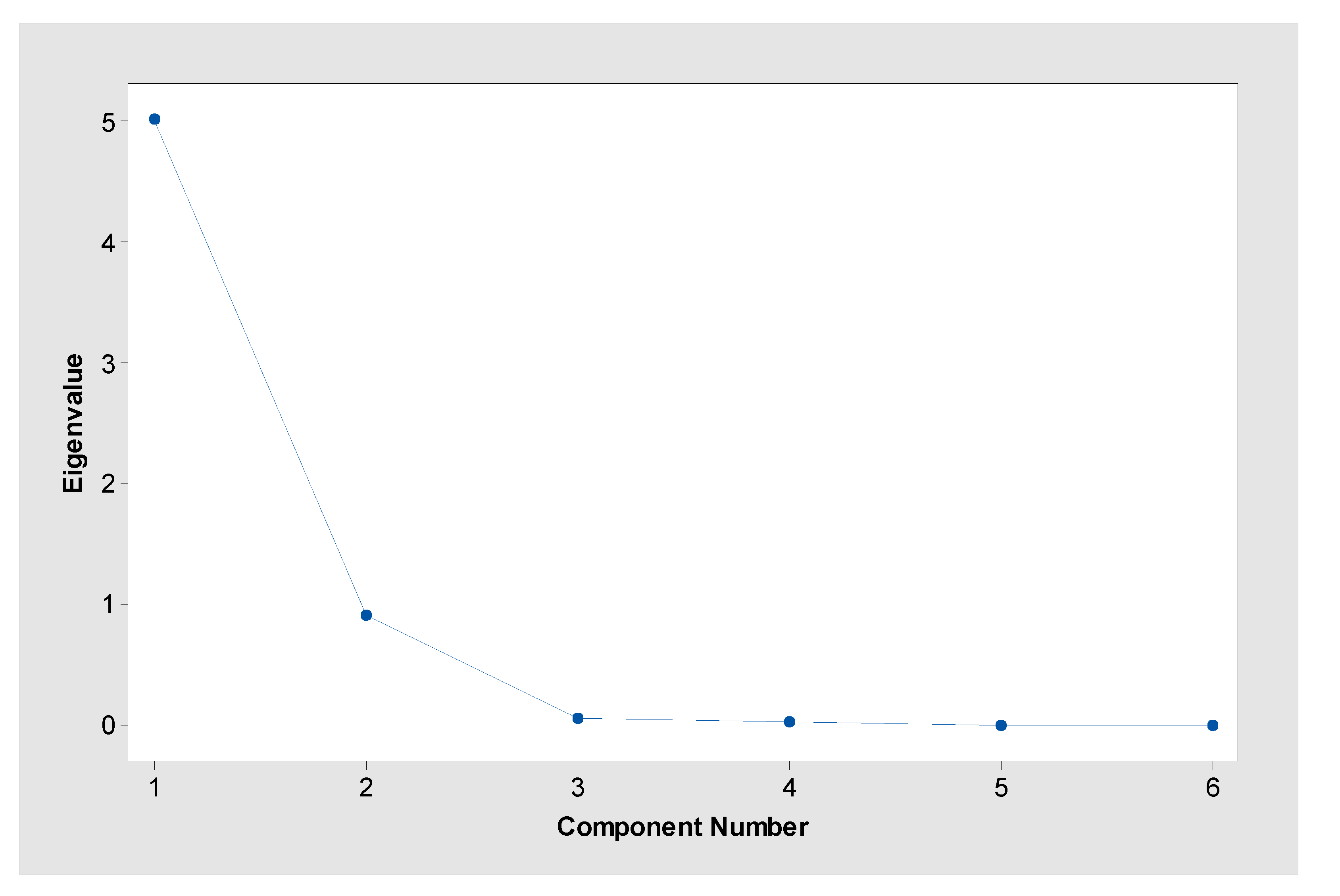
In this study, we perform PCA over the three scatterometer parameters mentioned above in both horizontal and vertical polarizations. Therefore, there are altogether 6 parameters (3 parameters × 2 polarizations). Six different regions around Antarctica where different features of ice/ocean classes are expected to exist are selected (Figure 1). Ten dates chosen for PCA are 1 December, 2016; 14 December, 2016; 30 December, 2016; 1 February, 2017; 15 February, 2017; 28 February, 2017; 2 May, 2017; 16 May, 2017; 30 May, 2017; and 7 October, 2017. There are 240,000 usable data points per parameter per day from all the six regions. Using Minitab, PC coefficients are generated from the six input parameters (

Table 1. Principal component coefficients for the 6 parameters used in the study. H and V are horizontal and vertical polarizations, Tb is brightness temperature, Gam is ϒ₀, and Sig is σ₀.

Coeff ► Parameters▼	Coeff 1	Coeff 2	Coeff 3
Tb_H	0.3623	−0.6015	−0.08589
Tb_V	0.3668	−0.5857	−0.1571
Gam_H	0.4379	0.1604	0.5315
Gam_V	0.4185	0.3493	−0.4514
Sig_H	0.4380	0.1602	0.5303
Sig_V	0.4186	0.3490	−0.4476

) and the Scree plot is given in Figure 2. Using these coefficients, we generate the required Principal Components. Even though the Scree plot suggests that only two components are good enough to explain maximum variability of the given data sample, we have retained three components in this analysis so that we can generate an RGB image.

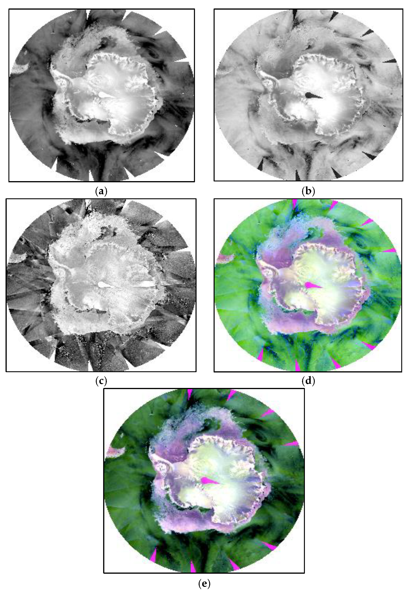
A sample of the generated principal components for a particular day is given in Figure 3 top panel (a–c). The first principal component (PC1) explains the largest percentage of total variance [20] followed by PC2 and PC3. The false-colour composite (FCC) image, shown at the bottom of Figure 3c, is generated using these three principal components as the input channels of red, green, and blue, respectively. In this FCC, regions with pinkish and greyish shades represent the sea ice area around Antarctica, while the green and black shades represent ocean. The FCC RGB image is transformed to hue, saturation, and value (HSV) colour space (Figure 3d) using the HSV transformation in ENVI software. This process replaces the value band with the high-resolution image, then it automatically resamples the hue and saturation bands to the high-resolution pixel size using cubic convolution technique. Ultimately, there is the final transformation of the image back to RGB colour space. The output RGB images will have the pixel size of the input high-resolution data.

3.2. Unsupervised Classification of Image

Next step is to segregate this sea ice region from the ocean pixels. To achieve this, we perform an unsupervised image classification, because there are no a priori training data to classify sea ice/ocean pixels. An unsupervised classifier does not require training data, and the classification is achieved by aggregating unknown pixels into different classes through natural grouping or clustering. The basic idea is that pixels belonging to a specific feature type should have nearby values in the measurement space compared to those pixels of different classes, which should be well separated [20].

Here, we have used the multivariate statistical analysis technique in ArcGIS, known as the Iso-cluster unsupervised classification using the HSV sharpened image described above. This technique is based on the Iterative Self-Organizing Data Analysis Technique (ISODATA) [20,22] algorithm of k-means clustering and, additionally, maximum likelihood classification, as well as a generalization analysis technique (majority filter) that replaces cells in a raster based on the majority of their contiguous neighbouring cells. This helps with the cleaning up of small erroneous data in the raster. Finally, sea ice boundary mask for the particular day is then applied, thereby reducing the ambiguous signals in regions where sea ice is not expected to exist.

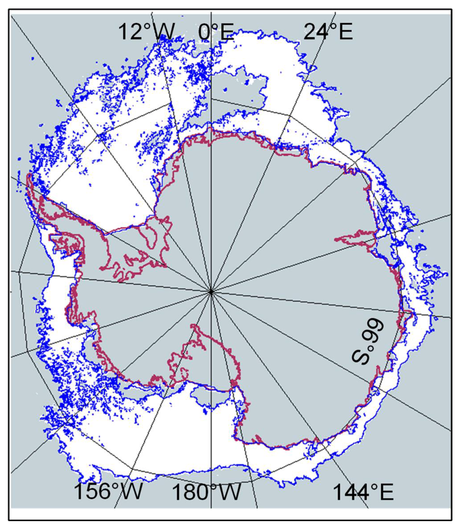
The sea ice map for 3 December 2016, determined from SCATSAT-1, is shown in Figure 4. The blue solid line is the sea ice boundary estimated from passive microwave data obtained by identifying pixels having more than 15% sea ice concentration. The formation of polynyas at different places around Antarctica is very well picked up by the method described here. This feature will be used in future for studying Antarctica polynya dynamics, particularly the Weddell Sea polynya. Detailed discussion on the comparison is given in the next section.

4. Comparison with Passive Microwave and SAR Data

4.1. Passive Microwave Data

For the purpose of comparison, the sea ice products, viz., SCATSAT-1, ASI, and BT sea ice maps are projected into South Polar stereographic 6.25 km spatial resolution (BT’s resolution—the coarsest of the three) using the layer stacking tool in ENVI.

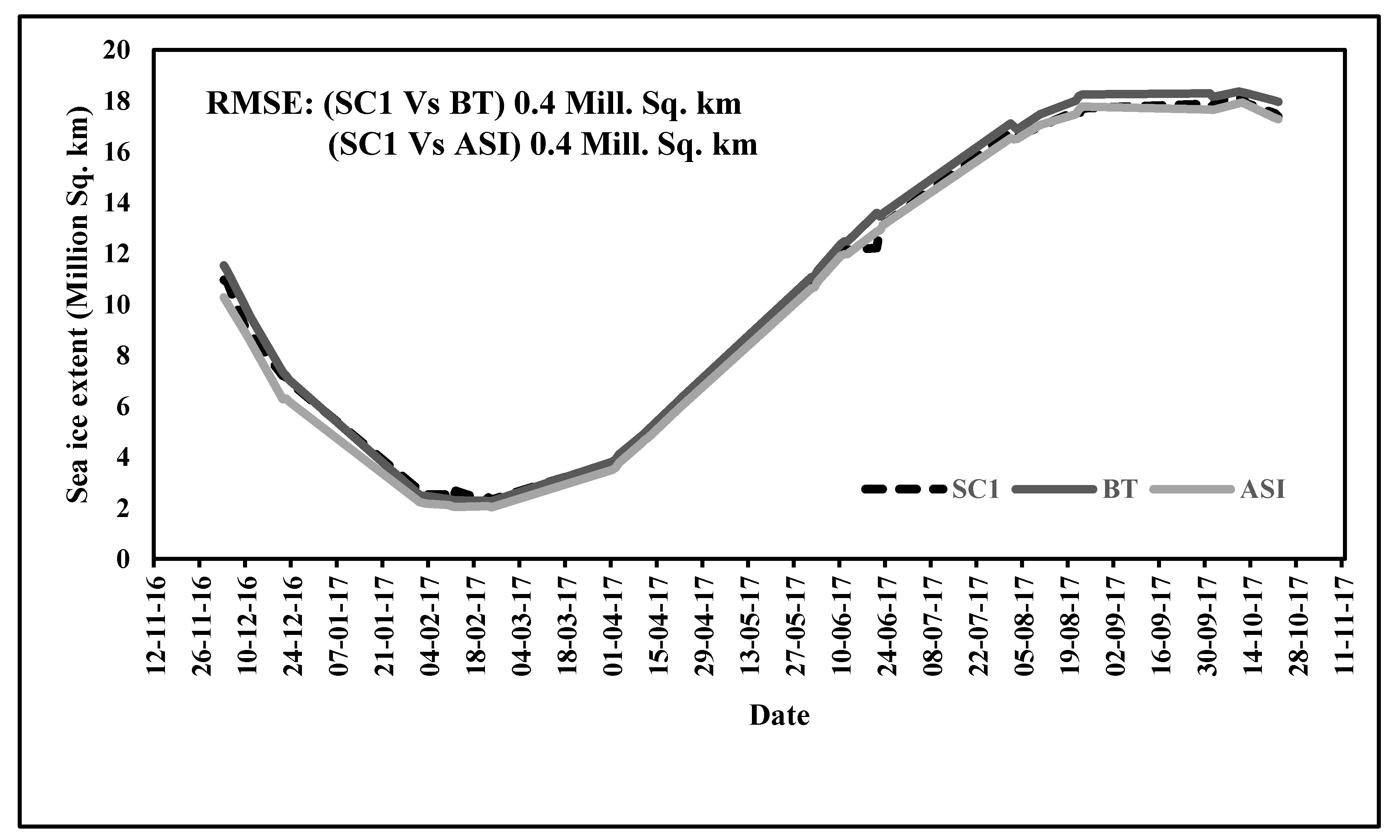
Forty eight dates from six different months (a few days in the beginning, middle, and end of each month) corresponding to one complete life-cycle of sea ice in the Antarctic oceans are chosen for comparative analysis. The sea ice extents derived from the above-mentioned three methods for these 48 days are shown in Figure 5. The root mean squared errors for (i) SCATSAT-1 vs Bootstrap and (ii) SCATSAT-1 vs ASI are ~0.4 Million km² in both the cases. Moreover, there is a high degree of correlation (r = 0.99) between the sea ice extents in both the comparisons.

In order to test the statistical significance of the results, we performed first the Fisher’s F-test (

Table 2. F-test statistics for (a) SCATSAT-1 and BT comparison, and (b) SCATSAT-1 and ASI.

(a)			(b)
	BT	SC1		ASI	SC1
Mean	10.51	10.25	Mean	10.00	10.25
Variance	37.33	35.09	Variance	36.32	35.09
Observations	48.00	48.00	Observations	48.00	48.00
df	47.00	47.00	df	47.00	47.00
F	1.06		F	1.03
P(F<=f) one-tail	0.42		P(F<=f) one-tail	0.45
F Critical one-tail	1.62		F Critical one-tail	1.62

) to check the variance between the pair of datasets (SC1 vs BT and SC1 vs ASI). Since the calculated F-value is smaller than the critical F-value, we accept the null hypothesis that the datasets have statistically equal variance. This test acts as a precursor for the next statistical test, the Student’s t-test to check the differences in population means of these datasets. We perform “two sample two-tail t-tests” to compare (a) SCATSAT-1(SC1) Versus Bootstrap (BT) and (b) SC1 Versus ASI. The t-test statistics are given in

Table 3. Student’s t-test results for (a) SCATSAT-1 (SC1) versus Bootstrap (BT) and (b) SC1 versus ASI.

(a)			(b)
	BT	SC1		ASI	SC1
Mean	10.51	10.25	Mean	10.00	10.25
Variance	37.33	35.09	Variance	36.32	35.09
Observations	48.00	48.00	Observations	48.00	48.00
Pooled Variance	36.21		Pooled Variance	35.71
Hypothesized Mean Difference	0.00		Hypothesized Mean Difference	0.00
df	94.00		df	94.00
t Stat	0.21		t Stat	-0.20
P(T<=t) two-tail	0.83		P(T<=t) two-tail	0.84
t Critical two-tail	1.99		t Critical two-tail	1.99

for both the cases. Absolute values of the calculated statistic (‘t stat’, in the tables) are smaller than the standard critical values for two-tail test (‘t Critical two-tail’). Hence, we cannot reject the null hypothesis, that is, the population means do not differ significantly. It may be noted here that all the statistical tests are done at 95% confidence level. Moreover, p-values are larger than 0.05 (the predefined significant level, alpha for the statistical tests).

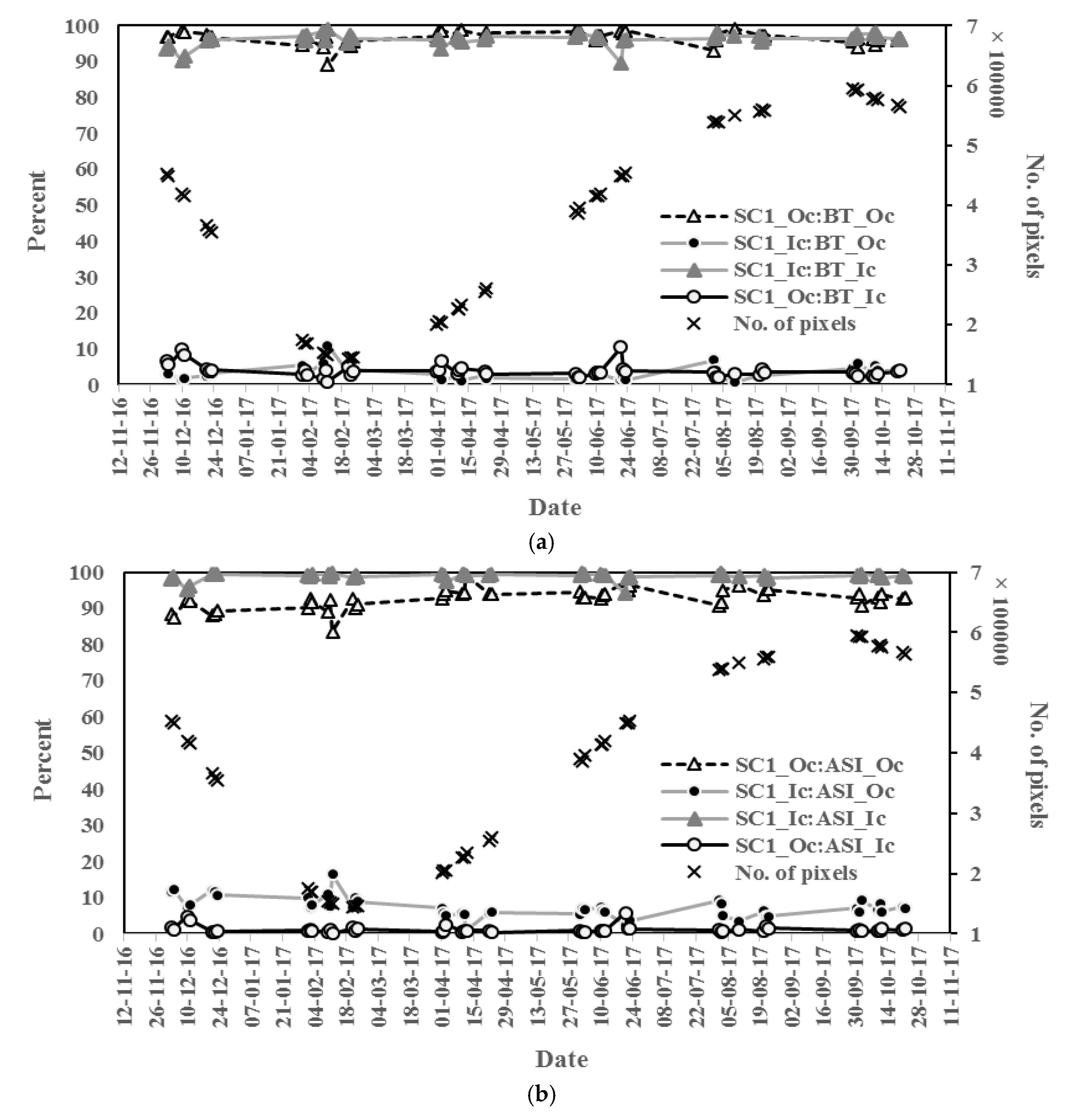
To further introspect into the matter, we perform a pixel-wise accuracy mapping between the estimated SCATSAT-1 SIE and the other two estimates (Figure 6). We map each pixel classified as either ocean or sea ice in the Bootstrap or ASI imagery against the pixel in the SCATSAT-1 imagery after re-projecting them into one common projection with a spatial resolution of 6.25 km. In the figure, ‘Oc’ represents ocean, and ‘Ic’, sea ice. Hence, SC1_Oc:BT_Oc represents the mapping accuracy for classifying pixels classified as ocean in Bootstrap algorithm as ocean in SCATSAT-1 estimation. Similarly, SC1_Ic:BT_Ic represents the sea ice classification accuracy in both the estimates. Number of pixels taken for comparison on each day is also plotted denoted by the ‘crosses’. There is an overall ice-to-ice mapping accuracy of 96% in SC1-BT and ~99% in SC1-ASI comparison. As shown in the plots, there are, however, some misclassifications as well (e.g., SC1_Oc:BT_Ic). Nonetheless, they are only ~10% or less in most of the cases.

4.2. SAR Data

We process the Sentinel-1 EW GRD data in the Sentinel Application Platform or SNAP. The detailed process is as follows:

(1)

Creation of a calibration look-up table for conversion of DN values to σ0,

(2)

Radiometric correction for removal of noise (3) speckle filtering using Lee-sigma filter,

(3)

Radiometric calibration to convert DN values to the corresponding σ0 using the look-up table, and

(4)

Geometric correction (ellipsoid correction) and re-projection to NSIDC South polar stereographic.

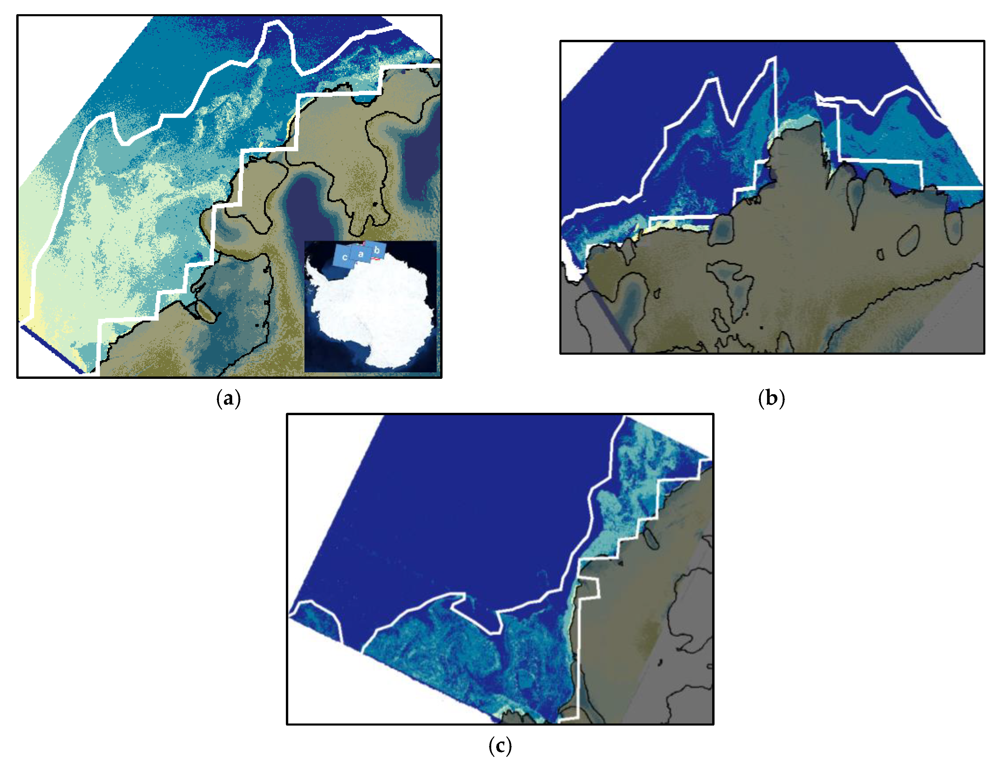
For this study, we have chosen three sites in East Antarctica (Figure 7). The white solid line is the sea ice edge estimated by our SCATSAT-1 algorithm for 20 January 2018. It is apparent our sea ice edge closely matches the SAR imageries. However, it may be noted here that the SAR scenes are one-minute observation of the region at a given local time and our SCATSAT-1 data are daily-averaged. Therefore, there will be some differences in the observation even though the “actual” sea ice edge looks similar to our estimated edge.

4.3. Ice Chart Shapefiles

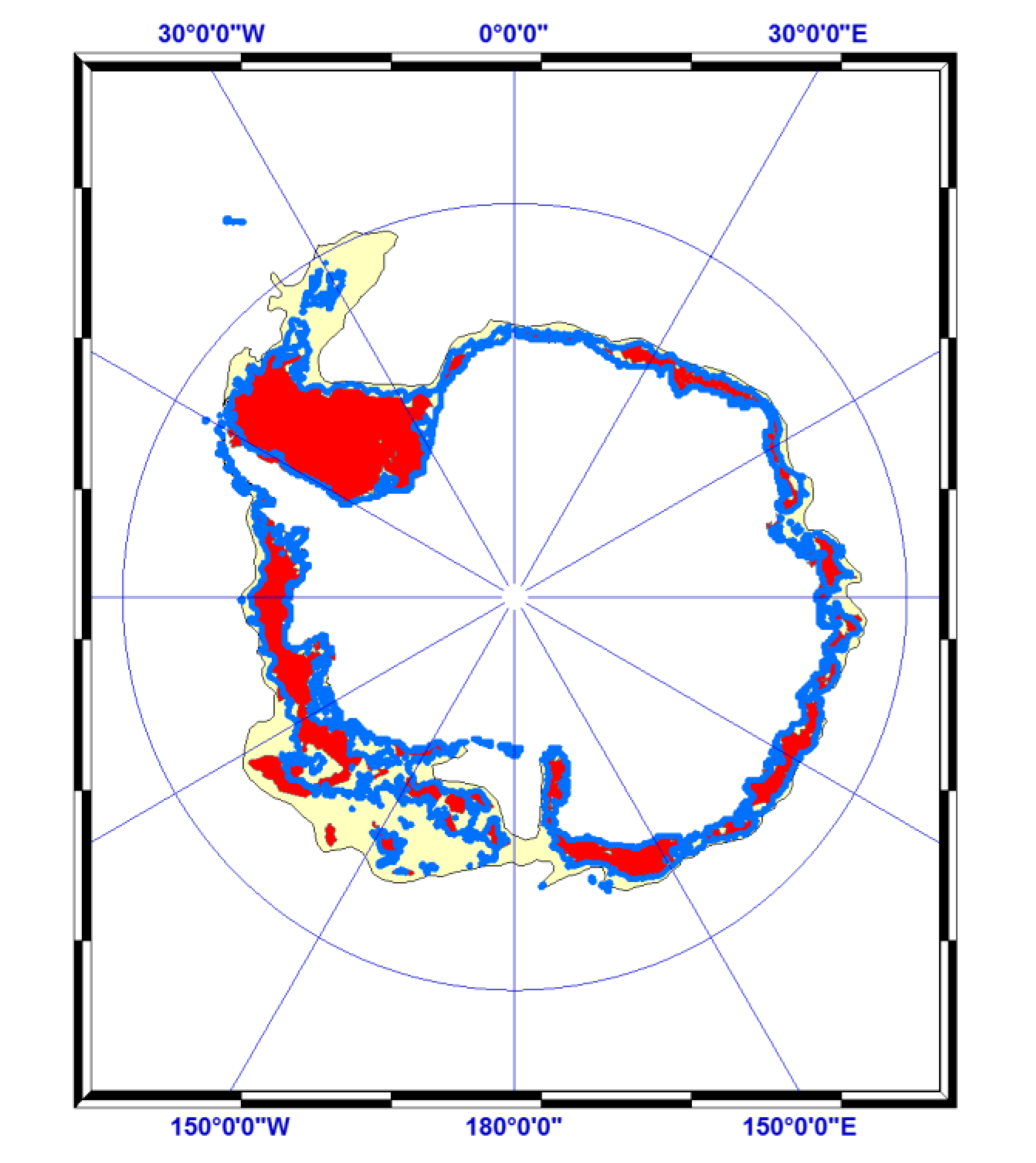
To complete the comparative analysis, we check the effectiveness of SCATSAT-1 sea ice algorithm in comparison to the ice edge obtained from an operational ice chart (Figure 8). We have compared the results for a few days but shown here the comparison for 20 January 2018.

The US NIC ice edge chart identifies the sea ice pack shown in red as those pixels having 8-10/10ths or greater of sea ice, while the Marginal Ice Zone (MIZ), where there is a lower concentration of sea ice, is shown in yellow. MIZ are the regions where ambiguities in the detection of sea ice edge using satellite remote sensing data can occur. This is due to the mixing of electromagnetic signatures returning from both sea ice and open ocean, and the errors can be even larger during summer melting season of sea ice [15].

It is apparent from this analysis that our SCATSAT-1 sea ice edge is in close match with the sea ice pack region as identified in the ice chart. We may notice distinctly that the Ross Sea polynya is clearly identified in our sea ice detection algorithm, as it is in the ice chart.

5. Conclusions

We made an attempt to develop an algorithm for the detection of sea ice in the Southern Oceans and to estimate the austral sea ice extent. The algorithm used the Indian Space Research Organisation’s SCATSAT-1 enhanced resolution data from the first year of operation at a spatial resolution of 2.225 km.

The algorithm used a combination of techniques such as the Principal Component Analysis and image classification technique (ISODATA k-means classifier). The sea ice estimates (edge and extent) from this method are found to have a high degree of correlation with other available high-quality sea ice products. Pixel-wise accuracy mapping reveals there is an overall ice-to-ice mapping accuracy of about 99% when compared with ARTIST Sea Ice (ASI)-derived sea ice extent and 96% when compared with Bootstrap. Ocean-to-ocean mapping accuracy is also high (in excess of 90%).

Moreover, in comparison with high resolution SAR and ice chart data, the algorithm tends to perform satisfactorily.

In the future, the algorithm will be applied to the detection of important Antarctic polynyas such as those occurring in Weddell Sea and Ross Sea, to study their dynamics.

References

- Comiso, J.C. Large-scale characteristics and variability of the global sea ice cover. In Sea Ice: An Introduction to Its Physics, Chemistry, Biology and Geology; Thomas, D., Dieckmann, G., Eds.; Blackwell Scientific: Oxford, UK, 2003; pp. 112–142. [Google Scholar]
- Gloersen, P.; Campbell, W.J.; Cavalieri, D.J.; Comiso, J.G.; Parkinson, C.L.; Zwally, H.J. Arctic and Antarctic Sea Ice, 1978–1987: Satellite Passive-Microwave Observations and Analysis (NASA Special Publication SP-511); NASA Goddard Space Flight Center: Greenbelt, MD, USA, 1992; p. 290. [Google Scholar]
- Lubin, D.; Massom, R. Sea ice. In Polar Remote Sensing, Vol-1-Atmosphere and Oceans; Springer-Praxis: Berlin/Heidelberg, Germany, 2006; pp. 309–609. [Google Scholar]
- Timmerman, R.; Beckmann, A.; Helmer, H.H. The role of sea ice in the fresh-water budget of the Weddell Sea, Antarctica. Ann. Glaciol. 2001, 33, 419–424. [Google Scholar] [CrossRef]
- Aagard, K.; Carmack, E.C. The role of sea ice and other fresh water in the Arctic circulation. J. Geophys. Res. 1989, 94, 14485–14498. [Google Scholar] [CrossRef]
- Martinson, D.G.; Iannuzzi, R.A. Antarctic ocean–ice inter- action: Implications from ocean bulk property distributions in the Weddell Gyre. In Antarctic Sea Ice: Physical Processes, Interactions and Variability (Antarctic Research Series 74); Jeffries, M.O., Ed.; American Geophysical Union: Washington, DC, USA, 1998; pp. 243–271. [Google Scholar]
- Remund, Q.P.; Long, D.G. Sea ice extent mapping using Ku band scatterometer data. J. Geophys. Res. 1999, 104, 11515–11527. [Google Scholar] [CrossRef]
- Remund, Q.P.; Long, D.G. A decade of QuikSCAT scatterometer sea ice extent data. IEEE Trans. Geosci. Remote Sens. 2014, 52, 4281–4290. [Google Scholar] [CrossRef]
- Cavalieri, D.J.; Gloersen, P.; Parkinson, C.L.; Comiso, J.C.; Zwally, H.J. Observed hemispheric asymmetry in global sea ice changes. Science 1997, 278, 1104–1106. [Google Scholar] [CrossRef]
- ISRO. SCATSAT-1 Wind Products (BETA Version) Released. 2018. Available online: https://www.isro.gov.in/SCATSAT-1-wind-products-beta-version-released (accessed on 22 January 2018).
- SCATSAT1 DP Team. SCATSAT-1 Level 4 Data Products Format Document, MDPD/SIPG; SC1/DP/L4FORMAT-DOC/V1.1/JUL2017; Space Applications Centre-ISRO: Ahmedabad, India, 2017. [Google Scholar]
- Spreen, G.; Kaleschke, L.; Heygster, G. Sea ice remote sensing using AMSR-E 89 GHz channels. J. Geophys. Res. 2008, 113. [Google Scholar] [CrossRef]
- Comiso, J.C. SSM/I Concentrations Using the Bootstrap Algorithm; NASA Reference Publication: Goddard Space Flight Center, Greenbelt, Maryland-20771, 1995. [Google Scholar]
- Zwally, H.J.; Comiso, J.C.; Parkinson, C.L.; Campbell, W.J.; Carsey, F.D.; Gloersen, P. Antarctic Sea Ice 1973–1976 from Satellite Passive Microwave Observations; NASA Special Publication: Goddard Space Flight Center, Greenbelt, Maryland, 1983; Volume 459, p. 206. [Google Scholar]
- Comiso, J.C.; Nishio, F. Trends in the sea ice cover using enhanced and compatible AMSR-E, SSM/I, and SMMR data. J. Geophys. Res. 2008, 113. [Google Scholar] [CrossRef]
- ESA Sentinel User Guide. 2018. Available online: https://sentinel.esa.int/web/sentinel/user-guides/sentinel-1-sar/resolutions/level-1-ground-range-detected (accessed on 8 January 2018).
- Rajak, D.R.; Singh, R.K.K.; Jayaprasad, P.; Oza, S.R.; Sharma, R.; Kumar, R. Sea ice occurrence probability data and its applications over the Antarctica. J. Geomat. 2015, 9, 193–197. [Google Scholar]
- Rothrock, D.A.; Thomas, D.R. Principal component analysis of satellite passive microwave data over sea ice. J. Geophys. Res. 1988, 93, 2321–2332. [Google Scholar] [CrossRef]
- Piwowar, J.M.; LeDrew, E.F. Principal components analysis of Arctic ice conditions between 1978 and 1987 as observed from the SMMR data record. Can. J. Remote Sens. 1996, 22, 390–403. [Google Scholar] [CrossRef]
- Lillesand, T.M.; Kiefer, R.W.; Chipman, J.W. Remote Sensing and Image Interpretation; John Wiley & Sons: New York, NY, USA, 2016; p. 756. [Google Scholar]
- Abdi, H.; Williams, L.J. Principal component analysis. Wiley Interdiscip. Rev. 2010, 2, 433–459. [Google Scholar] [CrossRef]
- Tou, J.T.; Gonzalez, R.C. Pattern Recognition Principles; Addison-Wesley: London, UK, 1974. [Google Scholar]
Figure 1.
Location map for the regions (marked in different colours) used in PCA overlaid on SCATSAT-1 backscatter (σ0) data.
Figure 2.
Scree plot from the principal component analysis.
Figure 3.
(a)–(c)- First (PC1), second (PC2), and third (PC3) principal component, respectively, generated from six scatterometer parameters; (d) false colour composite prepared using PC1, PC2, and PC3 as red, green, and blue channel, respectively; and (e) HSV-sharpened imaged of (d).
Figure 4.
Antarctic sea ice (white shade) extent from SCATSAT-1. Overlaid (blue contour) on the image is the sea ice boundary estimated from passive microwave (PMW) data for the same day (3 December 2016). The SIE obtained from SCATSAT-1 is ~10.7 × 10⁶ km2, while that from PMW is 10.3 × 10⁶ km2.
Figure 5.
Comparison of sea ice extents for the period December, 2016 to October, 2017 from SCATSAT-1, Bootstrap, and ASI algorithms. A correlation coefficient of 0.99 is obtained in both the comparisons, viz., SCATSAT-1 vs BT and SCATSAT-1 vs ASI.
Figure 6.
Pixel-wise mapping accuracy for the comparison between (
a) SCATSAT-1 (SC1) and Bootstrap (BT), and (
b) SC1 and ASI sea ice extent estimates. ‘Oc’ represents ocean and ‘Ic’ represents sea ice. Details are discussed in
Section 4.
Figure 7.
Comparison with Sentinel-1 SAR data. SCATSAT-1-derived sea ice extent (white contour) is overlaid over SAR imageries. Inset (a) shows the locations of these three imageries.
Figure 8.
Comparison of SCATSAT-1 sea ice edge (blue solid contour) with US NIC ice chart. Yellow regions are the Marginal Ice Zones, while red regions have higher sea ice concentration.