Observability and Performance Analysis of Velocity Measurements with Lever Arm Aided INS ^†

Abstract

In most autonomous vehicles the navigation subsystem is based on Inertial Navigation System (INS). Regardless of the INS grade, its navigation solution drifts in time. To avoid such a drift, the INS is fused with external sensor measurements. Recent publications show that the lever-arm, the relative position between the INS and aiding sensor, has influence on the navigation performance. Most published research in this field is focused on INS/GNSS fusion with GNSS position updates only where performance and analytical observability analysis were made to examine the consequence of vehicle maneuvers on the estimation of the lever-arm states. Yet, besides position updates, a variety of sensors measuring the vehicle velocity vector are available including GNSS and a Doppler velocity log. As in position measurements, when performing INS/velocity measurements fusion, the lever-arm must be taken account for. In this paper, performance analysis for velocity measurements with lever-arm aided INS is made for different maneuvers. Two error-states models are used in the analysis. Simulation results show the sensitivity of the error-states to lever arm and vehicle maneuver.

1. Introduction

Navigating air, sea and land vehicles using multi-sensor navigation systems has been subject to increasing interest in the literature. From the overgrowing need for high precision and reliable navigation systems and through the diverse potential for independence and automotive platforms, navigation based on multi-sensor fusion will allow to utilize the advantages of each individual sensor to optimize the process performance [1,2,3,4].

When performing this multi-sensor integration, one must take into account the effect of lever-arm, which is usually referred to the relative position between the sensors mounted on the vehicle. Publications show that the lever-arm has influence on the navigation performance and observability, of the integrated navigation system [5,6,7].

So far, however, there has been no discussion about the lever-arm effect in the case of velocity measurements update. Nowadays, a variety of velocity measurements sources are available and may be used to enhance navigation, especially in areas were GPS measurements are absence [5]. In this paper, the observability of lever-arm aided INS with velocity measurement is tested. Software simulations conducted to find the observable and unobservable subspaces for different maneuvers. Such a derivation is made for the 12 errors state model, where the position and lever-arm errors are not included in the error state, and additionally to the 15 errors state model, where the lever-arm error is included with three more error-state.

2. Problem Formulation

2.1. Kinematic Equation of Motion

In this section the navigation equations of motion and error-state model used in this study are introduced. In both models we omit the position states since they are not observable from velocity measurements [8]. For convenience, the local navigation reference frame was chosen to represent the velocity and attitude misalignment while the accelerometer and gyro biases are represented in the body reference frame. The navigation equations in the navigation frame [9,10]:

$${\dot{V}}^n=T_b^n{f}_{ib}^b+g^n-\left({\mathsf{\Omega }}_{en}^n+2{\mathsf{\Omega }}_{ie}^n\right)V^n,$$

(1)

$${\dot{T}}_b^n=T_b^n{\mathsf{\Omega }}_{ib}^b-\left({\mathsf{\Omega }}_{ie}^n+{\mathsf{\Omega }}_{en}^n\right)T_b^n.$$

(2)

where $V^n$ and $g^n$ are the velocity and gravitation vectors represented in the navigation frame, $T_b^n$ is the transformation matrix from body to navigation frame, $f_{ib}^b$ and ${\mathsf{\Omega }}_{ib}^b$ are the specific force and the skew-symmetric matrix of the angular velocity vector, respectively represented in the body frame. The notations used for reference frames are: i-frame (inertial), e-frame (earth fixed), b-frame (body) and n-frame (navigation).

2.2. Error States Models

The errors mechanization model for the navigation equations was considered as follow:

$${\widehat{V}}^n=V^n+\delta V^n,$$

(3)

$${\widehat{T}}_b^n=\left(I+\left[{\gamma }^n\times \right]\right)T_b^n,$$

(4)

$${\widehat{f}}_{ib}^b=f_{ib}^b+{\epsilon }_a+w_a,$$

(5)

$${\widehat{\omega }}_{ib}^b={\omega }_{ib}^b+{\epsilon }_g+w_g,$$

(6)

$${\widehat{l}}^b=l^b+\delta l^b.$$

(7)

where $\delta V^n$ and ${\gamma }^n$ are the velocity errors and attitude misalignment vectors respectively, $\left[{\gamma }^n\times \right]$ is the skew-symmetric matrix of ${\gamma }^n$, ${\widehat{f}}_{ib}^b$ and ${\widehat{\omega }}_{ib}^b$ are the specific force and gyro measurements, ${\epsilon }_a$ and $w_a$ are the accelerometer bias and random noise, ${\epsilon }_g$ and $w_g$ are the gyro bias and random noise, and $l^b$ is the lever-arm elements expressed in the body frame. The system dynamics can be written as

$$\delta \dot{x}=A\delta x+Gw,$$

(8)

where $\delta x$ is the error-state vector, $A$ is the system matrix, $w$ is the system noise vector and G is the system noise distribution matrix. Two error state models are implemented and compared as addressed in the following sections.

2.2.1. 12 Error State Model

The 12 error state model consists of the velocity, attitude, accelerometer bias and gyro bias error states. In the 12 error state model the lever-arm error is omitted and considered to be known and constant. This model is suitable when lever-arm elements estimation is done with a high confidence. In that case, the expected STD for the other elements in the vector should decrease.

When assuming constant biases, the corresponding linear model is given by [11]:

$$\delta {\dot{V}}^n=-\left[T_b^n{f}_{ib}^b\times \right]{\gamma }^n+T_b^n{\epsilon }_a+T_b^n{w}_a,$$

(9)

$${\dot{\gamma }}^n=-T_b^n{\mathsf{\Omega }}_{ib}^b{T}_b^n{}^T{\gamma }^n+T_b^n{\epsilon }_g+T_b^n{w}_g,$$

(10)

$${\dot{\epsilon }}_a=0,$$

(11)

$${\dot{\epsilon }}_g=0.$$

(12)

The error-state vector is then

$$\delta x_{12}={\left[\begin{array}{ccc}\delta v& \gamma & \begin{array}{cc}{\epsilon }_a& {\epsilon }_g\end{array}\end{array}\right]}^T$$

(13)

and the system dynamics in (8) can represent by

$$A_{12}=\left[\begin{array}{cc}\begin{array}{ccc}{0}_{3x3}& -\left[T_b^n{f}_{ib}^b\times \right]& T_b^n\\ 0_{3x3}& -T_b^n{\mathsf{\Omega }}_{ib}^b{T}_b^n{}^T& 0_{3x3}\\ 0_{3x3}& 0_{3x3}& 0_{3x3}\end{array}& \begin{array}{c}{0}_{3x3}\\ T_b^n\\ 0_{3x3}\end{array}\\ \begin{array}{ccc} 0_{3x3}& 0_{3x3}& 0_{3x3}\end{array}& 0_{3x3}\end{array}\right],$$

(14)

$$G_{12}=\left[\begin{array}{c}\begin{array}{cc}{T}_b^n& 0_{3x3}\\ 0_{3x3}& T_b^n\\ 0_{3x3}& 0_{3x3}\end{array}\\ \begin{array}{cc}{0}_{3x3}& 0_{3x3}\end{array}\end{array}\right].$$

(15)

2.2.2. 15 Error State Model

The 15 error state model contains all errors from the 12 error state model augmented with the lever-arm error-states, (which is now not considered to be constant). This model is suitable for situations where lever-arm elements are hard to evaluate. The model shares the same navigation equations and dynamic linear model as in the 12 error state model, with the addition of terms regarding the lever-arm error.

Let the additional lever-arm elements states modeled as constants

$$\delta {\dot{l}}^b=0,$$

(16)

Thus, the error-state vector is then

$$\delta x_{15}={\left[\begin{array}{ccc}\delta v& \gamma & \begin{array}{ccc}{\epsilon }_a& {\epsilon }_g& \delta l\end{array}\end{array}\right]}^T.$$

(17)

and the system dynamics in (8) can represent by

$$A_{15}=\left[\begin{array}{ccccc}{0}_{3x3}& -\left[T_b^n{f}_{ib}^b\times \right]& T_b^n& 0_{3x3}& 0_{3x3}\\ 0_{3x3}& -T_b^n{\mathsf{\Omega }}_{ib}^b{T}_b^n{}^T& 0_{3x3}& T_b^n& 0_{3x3}\\ 0_{3x3}& 0_{3x3}& 0_{3x3}& 0_{3x3}& 0_{3x3}\\ 0_{3x3}& 0_{3x3}& 0_{3x3}& 0_{3x3}& 0_{3x3}\\ 0_{3x3}& 0_{3x3}& 0_{3x3}& 0_{3x3}& 0_{3x3}\end{array}\right],$$

(18)

$$G_{15}=\left[\begin{array}{c}\begin{array}{cc}{T}_b^n& 0_{3x3}\\ 0_{3x3}& T_b^n\\ 0_{3x3}& 0_{3x3}\end{array}\\ \begin{array}{cc}{0}_{3x3}& 0_{3x3}\\ 0_{3x3}& 0_{3x3}\end{array}\end{array}\right],$$

(19)

2.3. Velocity Aiding

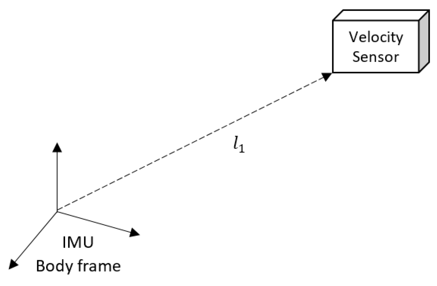
Consider a single level-armed velocity measurement sensor to an INS system as shown in Figure 1, were $l_1$ is the lever-arm. Those measurements can be modeled as:

$$V_1^n=V^n+T_b^n\left[{\omega }_{ib}^b\times \right]l^b$$

(20)

where $V_1^n$ represent the velocity measurement vector with lever-arm and ${\omega }_{ib}^b$ is the angular velocity vector. Let the measurement residual, the difference between the INS-based velocity and measurement vecloity, be

$$\delta V_1^n={\widehat{V}}_1^n-V_1^n,$$

(21)

then, using expressions (3)–(7) and (20), we obtain

$$\delta V_1^n=\delta V^n+\left(I+\left[{\gamma }^n\times \right]\right)T_b^n\left({\omega }_{ib}^b+{\epsilon }_g\right)\times \left(l^b+\delta l^b\right)-T_b^n{\omega }_{ib}^b\times l^b.$$

(22)

After rearranging and eliminating 2nd order error elements (22) reduces to

$$\delta V_1^n=\delta V^n-\left[T_b^n\left({\omega }_{ib}^b\times \right)l^b\times \right]{\gamma }^n-T_b^n\left[l^b\times \right]{\epsilon }_g+T_b^n{\omega }_{ib}^b\times \delta l^b.$$

(23)

Let $L^b=\left[l^b\times \right]$ and ${\mathsf{\Omega }}_{ib}^b=\left[{\omega }_{ib}^b\times \right]$, thus the velocity measurement estimation error can be written as:

$$\delta V_1^n=\delta V^n-\left[T_b^n{\mathsf{\Omega }}_{ib}^b{l}^b\times \right]{\gamma }^n-T_b^n{L}^b{\epsilon }_g+T_b^n{\mathsf{\Omega }}_{ib}^b\delta l^b.$$

(24)

The measurement model can be written as

$$\delta z=H\delta x+v$$

(25)

where $\delta z$ is the velocity measurement residual vector, $H$ is the measurements design matrix and$v$v is the measurements noise.

2.3.1. 12 Error State Model

Let a 12 error-state vector in (25), then the measurements matrix according to (24), after omitting lever-arm error coefficients, is

$$H_{12}=\left[\begin{array}{cc}\begin{array}{ccc}{I}_{3x3}& -\left(T_b^n{\mathsf{\Omega }}_{ib}^b{l}^b\times \right)& 0_{3x3}\end{array}& -T_b^n{L}^b\end{array}\right].$$

(26)

2.3.2. 15 Error State Model

Let a 15 error-state vector in (25), then the measurements matrix according to (24) is

$$H_{15}=\left[\begin{array}{cc}\begin{array}{ccc}{I}_{3x3}& -\left(T_b^n{\mathsf{\Omega }}_{ib}^b{l}^b\times \right)& 0_{3x3}\end{array}& \begin{array}{cc}-T_b^n{L}^b& T_b^n{\mathsf{\Omega }}_{ib}^b\end{array}\end{array}\right].$$

(27)

3. Results and Discussion

To test the observability properties of the models a variance software simulation was conducted. A low-grade IMU sensor was simulate at 100 Hz. The INS solution was corrected with EKF (Extended Kalman Filter) at 1 Hz using the velocity measurements. All measurements were assumed to be Gaussian white. The STD of the velocity measurements noise was set to 0.1 m/s, with lever arm of [1 0 0] in meters in the body frame. The accelerometer bias and noise STD were set to [−0.05 0.05 −0.1] and 0.01 in m/s², respectively. The gyro bias and noise STD were set to [−0.1 0.05 0.1] and 0.1 in °/s², respectively.

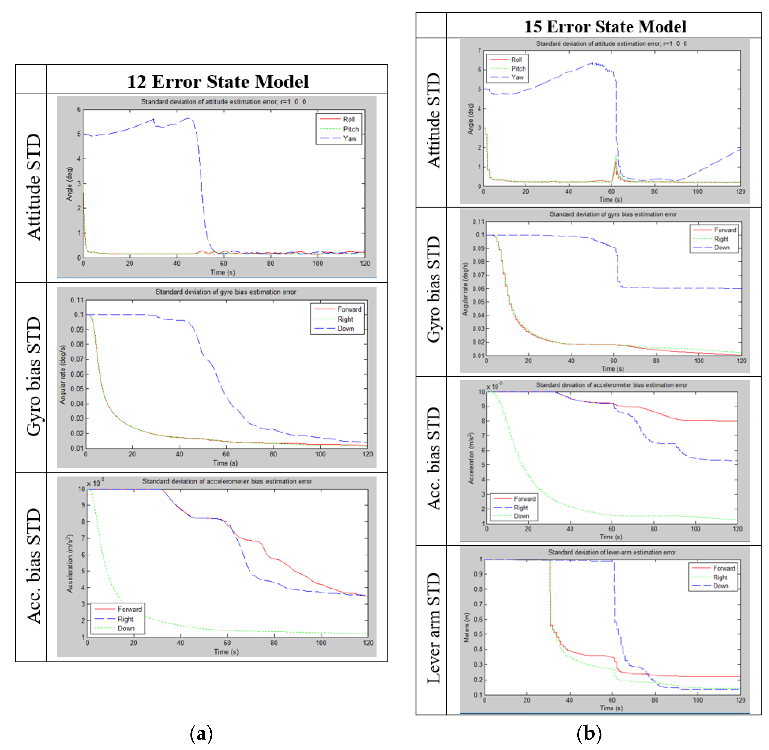
The simulation complete time of 120 s and tested 4 maneuvers—in the first 30 seconds the system was motionless, in 30–60 the system establish 1 complete round around Z axis, in 60–90 the system establish 1 complete round around X axis, and in 90–120 the system accelerated in X.

3.1. 12 Error State Model

Figure 2a shows the STD simulation results for the 12 error-state model. According to the attitude STD graph, both roll and pitch STD’s decreases from the beginning while the yaw STD decreases only when the system rotated around X. Similarly, the gyro bias STD is decreases rapidly for the horizontal components while the ‘Down’ component is significantly improve only when the systems experiencing changes in the vertical specific force while rotating around X. This behavior is opposite for the accelerometer bias STD when the ‘Down’ component start decreasing immediately while the horizontal components began to be reduced only when the system is experiencing changes in the rotation rate.

The findings here are equivalent to the description in [6], while here this results are related to the velocity measurement scenario, instead of the position, and with a comparison between the 12 and 15 error state models.

3.2. 15 Error State Model

Figure 2b shows the STD simulation results for the 15 error-state model. The STD values are decreasing slow and not as low as the 12 error state model due to the uncertainty in the lever-arm elements. This weaken the solution of the 15 error state model, especially in rotation maneuvers when the lever-arm is expressed in the measurements model. Using the 15 error state model though, the extraction of the lever arm elements is possible. As shown in Figure 2b, errors in lever-arm estimation reduced only when the system rotate, and the direction of the improvement is orthogonal to the rotation axis.

4. Conclusions

In this paper, the performance of lever-arm aided INS with velocity measurement is analyzed. 12 and 15 error-state models are compared to understand the implications of adding the lever-arm elements to the state vector.

Performance properties of all variables in the state vector drawn for different types of maneuvers. Simulation results showed that adding the lever-arm elements to the state vector is weaken the solution with slow convergence of the STD values, especially in stationary condition when no lever-arm improvement has occur. Nevertheless, having the lever-arm elements in the state vector can improve their estimation when system experience angular velocity. The direction of the improvement is orthogonal to the rotation axis.