Cost-Benefit Optimization of Sensor Networks for SHM Applications ^†

Abstract

Structural health monitoring (SHM) is aimed to obtain information about the structural integrity of a system, e.g., via the estimation of its mechanical properties through observations collected with a network of sensors. In the present work, we provide a method to optimally design sensor networks in terms of spatial configuration, number and accuracy of sensors. The utility of the sensor network is quantified through the expected Shannon information gain of the measurements with respect to the parameters to be estimated. At assigned number of sensors to be deployed over the structure, the optimal sensor placement problem is ruled by the objective function computed and maximized by combining surrogate models and stochastic optimization algorithms. For a general case, two formulations are introduced and compared: (i) the maximization of the information obtained through the measurements, given the appropriate constraints (i.e., identifiability, technological and budgetary ones); (ii) the maximization of the utility efficiency, defined as the ratio between the information provided by the sensor network and its cost. The method is applied to a large-scale structural problem, and the outcomes of the two different approaches are discussed.

1. Introduction

Structural Health Monitoring (SHM) allows to detect and estimate variations in the mechanical properties of structural and engineered systems [1,2] and, hence, make decisions about the actions needed to maintain or recover the overall structural safety [3]. Within a stochastic framework, the higher the SHM system effectiveness, the lower the uncertainties of the estimated quantities. The aim of the present work is the optimization of the SHM system, in terms of accuracy, number and spatial configuration of the sensors. Two main advantages can be therefore foreseen: first, the amount of information obtained from sensor measurements can be increased; second, the number of sensors can be reduced without sacrificing the information content. In this way, on one hand the overall cost of the SHM system can be reduced, on the other hand, as the amount of data to be analysed is cut down, the computational cost of the SHM method can be decreased, allowing for real-time applications (e.g., see [4]).

In the remainder of the paper, a theoretical introduction of the optimization formulation is given in Section 2. Then, its application to a structural problem is discussed in Section 3. Finally, in Section 4 some concluding remarks are gathered.

2. Theoretical Framework

Let us assume that the goal of the SHM system is the estimation of a set of parameters (e.g., mechanical properties, geometrical properties, damage indices) defined within an appropriate mathematical numerical model, used to predict the response of the structure to given loads. Within a Bayesian framework, the prior probability density function (pdf) $p\left(\theta \right)$ (where $\theta \in {\mathbb{R}}^{n_{\theta }}$ is the random vector of the $n_{\theta }$ parameters to be estimated) can be updated into the posterior pdf $p\left(\theta \right|\mathbf{y})$, when the measurements $\mathbf{y}\in {\mathbb{R}}^{n_{\mathbf{y}}}$ are collected through the sensor network. Following a Bayesian experimental design approach, the overall information provided by the measurements can be quantified using the information theory, as introduced in [5]. Applying these concepts to the problem of optimal sensor placement, a strategy based on the combination of surrogate models (see [6]) and stochastic optimization (see [7]), was introduced in [4,8]. Let us call $n_{\mathbf{y}}$ the number of measurements, $p_{ϵ}$ the pdf of the prediction error $ϵ$, and $\mathit{d}\in {\mathbb{R}}^{n_{\mathit{d}}}$ the design variables which provide the spatial configuration of the network on the structure. The optimal sensor placement configuration ${\mathit{d}}^{*}$ can be obtained by maximizing the expected Shannon information gain $U\left(\mathit{d}\right)$, see [4]; in doing this, parameters $n_{\mathbf{y}}$ and $p_{ϵ}$ are supposed to be fixed for a specific optimization problem.

In general, the expected Shannon information gain is a function of $\mathit{d}$, $n_{\mathbf{y}}$ and $p_{ϵ}$. The prediction error $ϵ={ϵ}_m+{ϵ}_n$ depends on both the model error ${ϵ}_m$ and the measurement noise ${ϵ}_n$. In [9], it was proven that the spatial correlation among different measurements, which is embedded into $p_{{ϵ}_m}$, affects the optimal sensor configuration ${\mathit{d}}^{*}$. On the other hand, if the environmental effects are neglected, the pdf of the measurement noise ${ϵ}_n$ can be directly linked to the employed sensors, as the probability model $p_{{ϵ}_n}$ depends on the sensor characteristics. The sensor network can be therefore optimized, in terms of spatial configuration, number and type of sensors, by maximizing the expected Shannon information gain according to:

$$({\mathit{d}}^{*},n_{\mathbf{y}}^{*},p_{{ϵ}_n}^{*})=argmax\left[U(\mathit{d},n_{\mathbf{y}},p_{{ϵ}_n})\right]$$

(1)

where $p_{{ϵ}_m}$ is instead supposed to be constant.

Assuming that ${ϵ}_n$ is sampled from a zero mean Gaussian pdf $p_{{ϵ}_n}=\mathcal{N}(\mathbf{0},{\Sigma }_n)$, where $\mathbf{0}\in {\mathbb{R}}^{n_{\mathbf{y}}}$ is the mean vector, and ${\Sigma }_n\in {\mathbb{R}}^{n_{\mathbf{y}}\times n_{\mathbf{y}}}$ is the covariance matrix, then $U=U(\mathit{d},n_{\mathbf{y}},{\Sigma }_n)$. For the sake of simplicity, we next assume that there is no correlation between measurements and so ${\Sigma }_n={\sigma }^2\mathbf{I}$, where $\sigma$ is the standard deviation of measurement noise and $\mathbf{I}\in {\mathbb{R}}^{n_{\mathbf{y}}\times n_{\mathbf{y}}}$ is the identity matrix. The optimization statement in Equation (1) thus becomes:

$$({\mathit{d}}^{*},n_{\mathbf{y}}^{*},{\sigma }^{*})=argmax\left[U(\mathit{d},n_{\mathbf{y}},\sigma )\right]$$

(2)

The function $\overline{U}=U({\mathit{d}}^{*},n_{\mathbf{y}},\sigma )$, corresponding to the maximum of the objective function for each value of $n_{\mathbf{y}}$ and $\sigma$, is computed for the corresponding optimal sensor configuration ${\mathit{d}}^{*}$. As ${\mathit{d}}^{*}$ depends on the choice of $\left\{n_{\mathbf{y}},\sigma \right\}$, then $\overline{U}=\overline{U}(n_{\mathbf{y}},\sigma )$ is implicitly a function of $n_{\mathbf{y}}$ and $\sigma$ only. It can be proven [10] and numerically shown [11] that $\overline{U}$ increases as the number of sensors gets higher (more information is provided by the SHM system). Moreover, if $\sigma$ increases then $\overline{U}$ decreases, since the structure response gets hidden by the measurement noise [12]. Thus, it follows that $\overline{U}$ is a monotonically increasing function of $n_{\mathbf{y}}$ and a monotonically decreasing function of $\sigma$: additional constraints need therefore to be handled in order to obtain the optimal solution of Equation (2).

Three types of constraints are here taken into account:

(a)

technological constraint $\sigma >{\sigma }_{best}$, with ${\sigma }_{best}$ designating the standard deviation of the measurement noise of the most accurate sensor available on the market, to provide measurements $\mathbf{y}$;

(b)

identifiability constraint $n_{\mathbf{y}}>n_{obs}$, with $n_{obs}$ designating the minimum number of measurements required to guarantee identifiability and observability of the parameters $\theta$ (see [2,13,14,15] );

(c)

cost constraint $C(n_{\mathbf{y}},\sigma )\le B$, with $C(n_{\mathbf{y}},\sigma )$ designating the cost model of the SHM system and B the maximum available budget.

The resulting constrained optimization problem is formulated as follows:

$$\begin{array}{cc}\hfill & ({\mathit{d}}^{*},n_{\mathbf{y}}^{*},{\sigma }^{*})=argmax\left[U(\mathit{d},n_{\mathbf{y}},\sigma )\right]\hfill \\ \hfill & \mathrm{subject}\mathrm{to}\left\{\begin{array}{c}{n}_{\mathbf{y}}>n_{obs}\hfill \\ \sigma >{\sigma }_{best}\hfill \\ C(n_{\mathbf{y}},\sigma )\le B\hfill \end{array}\right.\hfill \end{array}$$

(3)

As far as the cost model is concerned, the simplest formulation, includes a constant overall contribution $C_0$, which takes into account the cost of data acquisition hardware, database, assemblage, etc., and a variable contribution, which takes instead into account the cost of the sensors. The associated expression is:

$$C(n_{\mathbf{y}},\sigma )=C_0+c\left(\sigma \right)n_{\mathbf{y}}$$

(4)

where $c\left(\sigma \right)$ is the cost per unit sensor.

One possible approach for solving the optimization problem would consist in defining a new design variable to account for $n_{\mathbf{y}}$ and $\sigma$; next, the optimal solution is obtained by applying an optimization algorithm for stochastic problems, like the Covariance Matrix Adaptation-Evolution Strategy [7]. When only a limited number of sensor types is available, an alternative approach is based on the computation of the function $\overline{U}=U({\mathit{d}}^{*},n_{\mathbf{y}},\sigma )=U(n_{\mathbf{y}},\sigma )$ on a set of points $\{n_{\mathbf{y}},\sigma \}$, as shown in Section 3.

The optimization problem introduced in Equation (3) allows to design a sensor network such that the provided information is maximized, given a certain budget B. Following a usual method in decision making strategies (see [16]), an alternative optimization rationale would be to maximize the ratio between the expected Shannon information gain and the cost of the SHM system, in a sort of cost-benefit analysis. Thus, the following utility-cost index (UCI) is defined:

$$\mathrm{UCI}(\mathit{d},n_{\mathbf{y}},\sigma )=\frac{U(\mathit{d},n_{\mathbf{y}},\sigma )}{C(n_{\mathbf{y}},\sigma )}$$

(5)

where the associated measurement unit is [nat/€], [nat] being natural unit of information. The resulting optimization problem then becomes:

$$\begin{array}{cc}\hfill & ({\mathit{d}}^{*},n_{\mathbf{y}}^{*},{\sigma }^{*})=argmax\left[\mathrm{UCI}(\mathit{d},n_{\mathbf{y}},\sigma )\right]\hfill \\ \hfill & \mathrm{subject}\mathrm{to}\left\{\begin{array}{c}{n}_{\mathbf{y}}>n_{obs}\hfill \\ \sigma >{\sigma }_{best}\hfill \\ C(n_{\mathbf{y}},\sigma )\le B\hfill \end{array}\right.\hfill \end{array}$$

(6)

The above formulation allows to obtain the most efficient SHM design, i.e., to maximize the information per unitary cost.

As regards the solution of the optimization problem, the objective function to be maximized turns out to be now $\overline{\mathrm{UCI}}=\mathrm{UCI}({\mathit{d}}^{*},n_{\mathbf{y}},\sigma )=\mathrm{UCI}(n_{\mathbf{y}},\sigma )$, where ${\mathit{d}}^{*}$ is the optimal sensor configuration, for each value of $n_{\mathbf{y}}$ and $\sigma$.

The application of the two formulations defined in Equations (3) and (6) to the optimal design of a SHM system is presented in Section 3.

3. Results

The method presented in Section 2 is applied to the Pirelli tower, a 130 m tall building in Milan. The associated finite element model features a total number of 4106 nodes, each one with 6 degrees of freedom, i.e., the displacement components $u_{x_1}$, $u_{x_2}$ and $u_{x_3}$ along the three axes $x_1$, $x_2$ and $x_3$ of an orthonormal reference frame and the rotation components ${\phi }_{x_1}$, ${\phi }_{x_2}$ and ${\phi }_{x_3}$ about the same axes. For further details on the model, the reader may refer to [17]. We herein assume that measurements can be either displacements or rotations; $n_{\theta }=6$ parameters, including both geometrical and mechanical properties, ought to be inferred (see [8] for further details on the choice of the parameters).

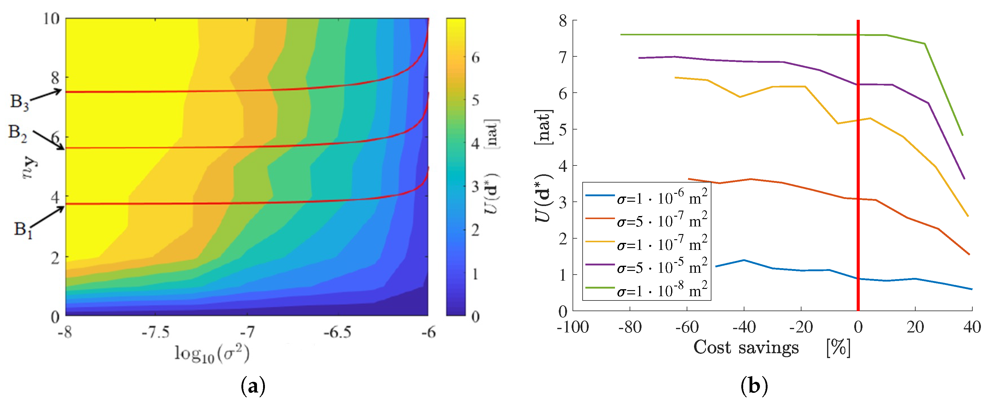
In Figure 1a, the contour plot of the objective function $\overline{U}(n_{\mathbf{y}},\sigma )=U({\mathit{d}}^{*},n_{\mathbf{y}},\sigma )$ is shown at varying number $n_{\mathbf{y}}$ and accuracy of the sensors (measured through $\sigma$). As previously discussed, the plot shows that the maximum value of the expected Shannon information gain increases as $n_{\mathbf{y}}$ gets higher and as the standard deviations decreases. It can be also observed that the increase in the expected Shannon information gain due to each additional measurement gets lower as more measurements are considered. In other words, the derivative $\frac{\partial U}{\partial n_{\mathbf{y}}}$ of the expected Shannon information gain with respect to the number of sensors is a decreasing function of $n_{\mathbf{y}}$. Interpreting the optimization problem within a decision-making view, it is interesting to underline that this behaviour corresponds to the so-called “law of diminishing marginal utility” (also known as Gossen’s First Law [18]), which was proposed for problems of resources allocation optimization. This law states that the marginal utility of a certain system, due to an additional unit, decreases as the supply of units increases. In the current problem of optimal SHM system design, the utility, i.e., the benefit of the sensor network is quantified by the expected Shannon information gain (see Section 2), and the unit is represented by each measurement.

If the cost model defined in Equation (4) is employed, the red lines in Figure 1a represent different budget constraints, i.e., the solutions $\left\{\sigma n_{\mathbf{y}}\right\}$ of the equation $B=C_0+c\left(\sigma \right)n_{\mathbf{y}}$, with B being the available budget (in the example $B_1=2000$ €, $B_2=2500$ €, $B_3=3000$ €). This graph allows the designer to choose the optimal SHM sensor network characteristics ${\sigma }^{*}$ and $n_{\mathbf{y}}^{*}$ and the associated optimal configuration ${\mathit{d}}^{*}$, which corresponds to the maximum $U(\mathit{d},n_{\mathbf{y}},\sigma )$: it is worth noting that in this case the solution is basically ruled by the budget constraint. A discussion about the optimal configurations ${\mathit{d}}^{*}$ obtained through the optimization procedure can be found in [8].

A different approach for decision making is to define a Pareto front for $U\left(\mathit{d}\right)$ versus cost savings, as shown in Figure 1b: each line here represents the optimal design for a certain standard deviation $\sigma$, i.e., a certain type of sensors. Along the x-axis the cost saving is represented, which is defined as the cost function normalized with respect to the chosen budget; the vertical straight line represents the budget B. Any design point located on the left of each line represents a non-optimal solution, i.e., the associated cost does not correspond to the best choice of $\left\{\mathit{d}{n}_{\mathbf{y}}\sigma \right\}$.

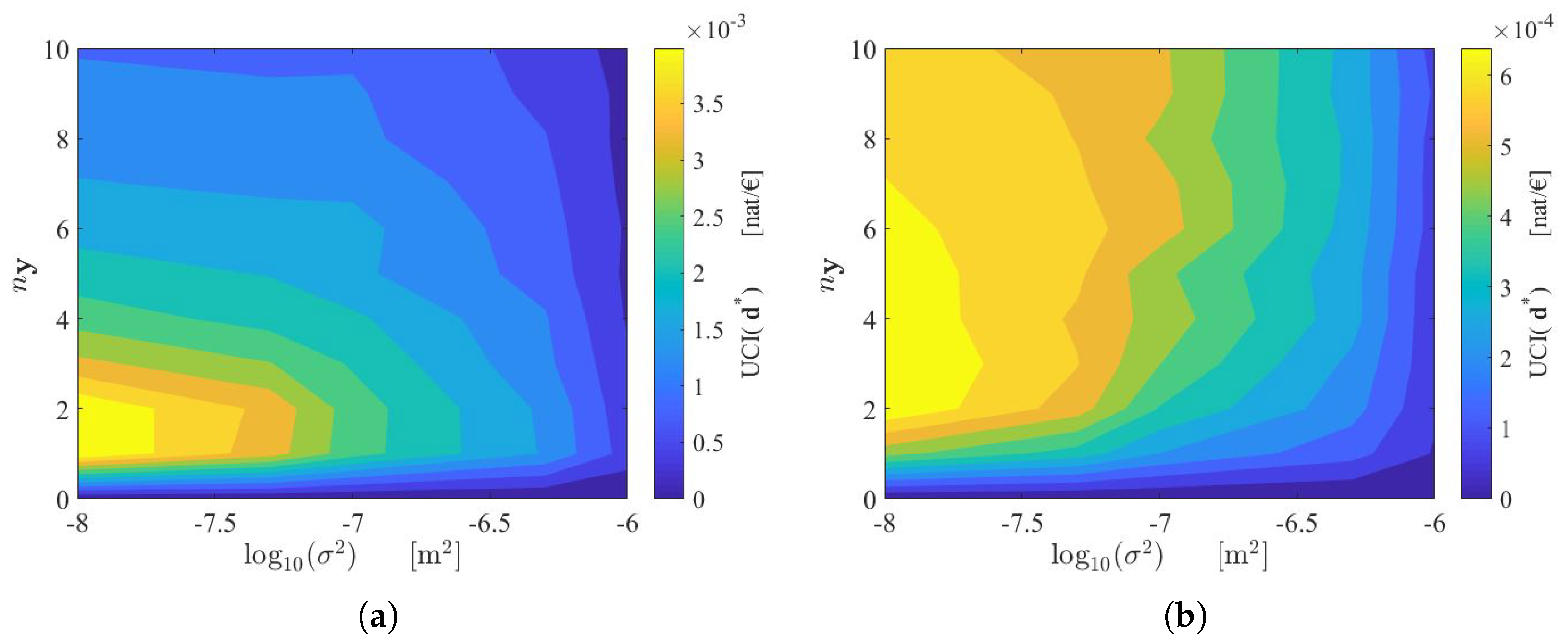
The alternative design optimization approach defined in Equation (6) is based on the maximization of the ratio $UCI(n_{\mathbf{y}},\sigma )=\frac{\overline{U}(n_{\mathbf{y}},\sigma )}{C(n_{\mathbf{y}},\sigma )}$. The resulting optimal solution obviously depends on the cost model: in Figure 2a the SHM system is supposed to have a lower cost $C_0=500$ €; in Figure 2b the SHM system is supposed to have a higher cost $C_0=1000$ €. In both cases, the most efficient allocation of resources is obtained if the best sensors, in terms of measurement noise, are chosen; the optimal number of sensors depends instead on the cost model: the higher $C_0$, the higher $n_{\mathbf{y}}^{*}$.

It is worth noting that, while the function $\overline{U}(n_{\mathbf{y}},\sigma )$ always increases with $n_{\mathbf{y}}$ and $\sigma$, the function $\overline{UCI}(n_{\mathbf{y}},\sigma )$ presents a maximum for a finite value of $n_{\mathbf{y}}$. As previously discussed, the increase in information associated with each additional sensor decreases as more sensors are considered: from a cost-benefit point of view, it is therefore worthless to add sensors, i.e., to increase the SHM cost, if the associated additional benefit (the additional expected Shannon information gain) becomes too low.

4. Conclusions

In the present work, a strategy to optimally design sensor networks for SHM applications, in terms of spatial configuration, accuracy and number of sensors, has been introduced. Two optimization formulations have been proposed, related either to the maximization of the expected Shannon information gain or to the maximization of the ratio between the information and the cost of the SHM system. The application of the two strategies to a large-scale structural problem has been discussed, highlighting the effect of the cost budget on the optimal solution. A Pareto front approach has been also discussed, allowing to obtain a prompt tool for the SHM system design.

References

1. Balageas, D.; Fritzen, C.P.; Güemes, A. Structural Health Monitoring; John Wiley & Sons: Hoboken, NJ, USA, 2010; Volume 90. [Google Scholar]
2. Yuen, K.V. Bayesian Methods for Structural Dynamics and Civil Engineering; John Wiley & Sons: Hoboken, NJ, USA, 2010. [Google Scholar]
3. Achenbach, J.D. Structural health monitoring—What is the prescription? Mech. Res. Commun. 2009, 36, 137–142. [Google Scholar] [CrossRef]
4. Capellari, G.; Chatzi, E.; Mariani, S. An optimal sensor placement method for SHM based on Bayesian experimental design and Polynomial Chaos Expansion. In Proceedings of the VII European Congress on Computational Methods in Applied Sciences and Engineering, Crete Island, Greece, 5–10 June 2016; Volume 3, pp. 6272–6282. [Google Scholar]
5. Lindley, D.V. On a measure of the information provided by an experiment. Ann. Math. Stat. 1956, 27, 986–1005. [Google Scholar] [CrossRef]
6. Huan, X.; Marzouk, Y.M. Simulation-based optimal Bayesian experimental design for nonlinear systems. J. Comput. Phys. 2013, 232, 288–317. [Google Scholar] [CrossRef]
7. Hansen, N. The CMA evolution strategy: A comparing review. In Towards a New Evolutionary Computation. Advances on Estimation of Distribution Algorithms; Lozano, J., Larranaga, P., Inza, I., Bengoetxea, E., Eds.; Springer: Berlin, Germany, 2006; pp. 75–102. [Google Scholar]
8. Capellari, G.; Chatzi, E.; Mariani, S. SHM network-optimization through Bayesian experimental design. Submitted.
9. Papadimitriou, C.; Lombaert, G. The effect of prediction error correlation on optimal sensor placement in structural dynamics. Mech. Syst. Signal Process. 2012, 28, 105–127. [Google Scholar] [CrossRef]
10. Papadimitriou, C.; Beck, J.L.; Au, S.K. Entropy-based optimal sensor location for structural model updating. J. Vib. Control 2000, 6, 781–800. [Google Scholar] [CrossRef]
11. Capellari, G.; Chatzi, E.; Mariani, S.; Azam, S.E. Optimal design of sensor networks for damage detection. Procedia Eng. 2017, 199, 1864–1869. [Google Scholar] [CrossRef]
12. Capellari, G.; Chatzi, E.; Mariani, S. Optimal sensor placement through Bayesian experimental design: Effect of measurement noise and number of sensors. Proceedings 2017, 1, 41. [Google Scholar] [CrossRef]
13. Katafygiotis, L.S.; Beck, J.L. Updating models and their uncertainties. II: Model identifiability. J. Eng. Mech. 1998, 124, 463–467. [Google Scholar] [CrossRef]
14. Chatzis, M.N.; Chatzi, E.N.; Smyth, A.W. On the observability and identifiability of nonlinear structural and mechanical systems. Struct. Control Health Monit. 2015, 22, 574–593. [Google Scholar] [CrossRef]
15. Capellari, G.; Chatzi, E.; Mariani, S. Parameter identifiability through information theory. In Proceedings of the 2nd ECCOMAS Thematic Conference on Uncertainty Quantification in Computational Sciences and Engineering, Rhodes Island, Greece, 15–17 June 2017. [Google Scholar]
16. Parnell, G.S.; Driscoll, P.J.; Henderson, D.L. Decision Making in Systems Engineering and Management; John Wiley & Sons: Hoboken, NJ, USA, 2011; Volume 81. [Google Scholar]
17. Barbella, G. Frequency Domain Analysis of Slender Structural Systems under Turbulent wind Excitation. Ph.D. Thesis, Doctoral School in Structural, Seismic and Geotechnic Engineering, Politecnico di Milano, Milan, Italy, 2009. [Google Scholar]
18. Gossen, H.H. The Laws of Human Relations and the Rules of Human Action Derived Therefrom; Mit Press: Cambridge, MA, USA, 1983. [Google Scholar]
Figure 1. (a) Contour plot of U ¯ ( n y , σ ) , where lines represents the budget constraints B = C ( σ , n y ) , with B 1 = 2000 €, B 1 = 2500 €, B 1 = 3000 €; (b) Pareto front of the expected Shannon information gain with respect to the SHM system cost.
Proceedings 02 00132 g001
Figure 2. Contour plot of U C I ( d * , n y , σ ) = U ¯ ( d * , n y , σ ) C ( n y , σ ) , with (a) C 0 = 500 € and (b) C 0 = 1000 €.
Proceedings 02 00132 g002
Publisher’s Note: MDPI stays neutral with regard to jurisdictional claims in published maps and institutional affiliations.