Transferable Deep Features for Keyword Spotting ^†

Abstract

Deep features, defined as the activations of hidden layers of a neural network, have given promising results applied to various vision tasks. In this paper, we explore the usefulness and transferability of deep features, applied in the context of the problem of keyword spotting (KWS). We use a state-of-the-art deep convolutional network to extract deep features. The optimal parameters concerning their application are subsequently studied: the impact of the choice of hidden layer, the impact of applying dimensionality reduction with a manifold learning technique, as well as the choice of dissimilarity measure used to retrieve relevant word images. Extensive numerical results show that deep features lead to state-of-the-art KWS performance, even when the test and training set come from different document collections.

1. Introduction and Related Work

Keyword spotting (KWS) is essentially the problem of image retrieval, cast on the context of collections of document, line and word images [1]. Depending on whether the scanned document is pre-segmented, either manually or automatically, into line or word tokens, an important taxonomy of KWS methods is in (line or word) segmentation-based and segmentation-free methods. Not surprisingly, learning-based methods are in general better performing than learning-free KWS methods [1]. The vast majority of recently proposed learning-based methods includes deep learning-based methods, which seem to have dominated this field as well [1,2,3].

In the context of KWS, the typical use of deep neural networks involves first training the model on pairs of segmented word or line images and annotations. Subsequently, using a feed-forward pass given an input word image, a descriptor is produced on the network output layer. The descriptor is then compared to descriptors of other words to give a sorted relevance list. It has however been noted that layers other than the output layer can be used to produce features. These features, corresponding to one (or more) hidden layers of the network, have been commonly known as deep features [4] in the literature (or hypercolumns [3,5], when more than one layer activations are combined). In other machine vision tasks, deep features have often led to superior results compared to the standard use of the network [4]. This is due to their being able to capture more abstract traits of the input [6]. This observation has inspired Zoning-Aggregated Hypercolumn (ZAH) features, proposed in [3], where deep features are extracted, processed and applied on a KWS task.

In this work, we use PHOCnet [2] as our model of reference. PHOCnet is a Deep Convolutional Network that has recently been proposed for KWS. We use PHOCnet to produce network outputs, i.e., using it as was originally intended, as well as to extract deep features suitable for the KWS task. With extensive numerical experiments, we validate the usefulness of deep features on various different setups for KWS. Furthermore, we show that deep features are much more transferable compared to simply using the network output. Even when the model seems to overfit on a particular training collection (an aspect that seems to have been overlooked on various recent works that nevertheless report very high performance figures [1]), deep features by comparison exhibit much better generality, in the sense of being applicable to a test set that comes from a different collection than the training set.

Another parameter that we explore is the value of combining manifold learning with the extracted features [7,8]. The intuition behind manifold learning methods is that data empirically lie on low-dimensional manifolds that span a relatively low volume of the original space. This hypothesis, commonly known as manifold hypothesis, has led to a series of methods that attempt to estimate the characteristic of the data manifold. We use the recently proposed t-SNE manifold learning method in this work. t-SNE has shown to be successful and enjoys a number of benefits—for example, it has shown to be robust to the so-called crowding problem (embedding coordinates crowding around zero) [7]. We show that using manifold learning to reduce the dimensionality of our features leads to increased KWS performance.

Furthermore, the question of which dissimilarity measure is more suitable for descriptor comparison is explored. As an alternative to the Euclidean distance, the Bray-Curtis dissimilarity (BC) has recently been employed in the context of keyword spotting [2,9]. We compare BC with the Euclidean distance, with and without applying L2-normalization before evaluation. Numerical experiments show that the L2-normalized Euclidean distance gives the best KWS results.

The remainder of this paper is organized as follows. In Section 2 we describe the employed pipeline to produce transferable deep features. In Section 3 we present numerical results comparing various setups of the proposed pipeline on KWS trials. We close the paper with Section 4 where we summarize our conclusions.

2. Method and Model Parameters

We assume a Query-by-Example (QbE) segmentation-based KWS scenario and the Mean Average Precision (MAP) evaluation metric [1]. This means that all data-both training and test- are segmented word images, and queries are word images as well. The core of the proposed method consists of using a CNN as a feature extractor. We have used PHOCnet [2], a CNN architecture recently proposed for segmentation-based KWS. PHOCnet was the best performing model on the recent ICFHR 2016 KWS competition (unpenalized MAP scenario) [1]. After having trained the CNN, the extracted Deep Features are defined simply as the activations of a hidden model layer, when a specific word image input is provided. Given all word images, plus the query, we thus create descriptors—one for each word image—based on deep features. These descriptors are typically of high dimensionality, with the exact number of the latter depending on the number of neurons per hidden layer. For example, the dimensionality of the features generated from layer $spp5$ (the closest to network input) is 10,752. Hence, a dimensionality reduction method can be applied to reduce the dimensionality of the descriptor. The final descriptors can then be compared using some measure of dissimilarity, in order to provide the retrieved query list. In the following subsections we explain these steps in more detail.

2.1. Neural Network Architecture and Deep Features

PHOCnet is a standard feed-forward neural network. The word image to be processed is fed to the network input, with information flowing first through a number of alternating standard convolutional and max pooling layers. The size of all these layers depends on the size of the input image. The last convolutional layer is then fed to a spatial pyramid max pooling layer (SPP) [10]. The SPP layer (referred to as $spp5$) produces a fixed-size output given a variable-size input, as it processes input from the previous layer after partitioning it into a hierarchy of grids of variable resolution ($4\times 4,2\times 2,1\times 1$). The SPP property of producing a fixed-size output regardless of the input, is in a way inherited by the whole model. In this manner, there is no need either to scale the input image to a fixed size or perform some manual zoning step afterwards, as done in [3] for example. The output of the SPP is fed to two fully connected layers, coupled with ReLU non-linearities (referred to as $relu6$, $relu7$). The final layer is structured in a manner to reflect the structure of a Pyramidal Histogram of Character (PHOC) vector [11]. PHOC variates capture information about the word, in the form of a set of word attributes. Each output neuron is coupled with sigmoid nonlinearities, producing an output vector with values ranging between 0 and 1. Regarding further details on the network architecture, as well as details on how training is performed (parameters, number of iterations, use of dropout, etc.), the reader is referred to the original publication [2]. All layers between the input layer and the SPP layer are of variable size, as they depend on the input word image size. Deep features extracted using activations of these layers would hence be not directly comparable to one another, as each one would lie on a space of different dimensionality. For that reason, we cannot extract useful deep features from these layers (at least without applying some postprocessing scheme to make them comparable, a question which we shall not explore in this paper). Therefore, we use $spp5$, $relu6$ and $relu7$ to extract deep features.

2.2. Manifold Learning

We use t-SNE as our non-linear manifold learning technique of choice [7]. In t-SNE, the goal is to minimize the divergence between pairwise similarity distributions of input points and the low-dimensional embedded points. The N input points are denoted as ${\left\{x_i\right\}}_{i=1}^N$ and their corresponding embeddings are denoted as ${\left\{y_i\right\}}_{i=1}^N$. The joint probability $p_{ij}$ that measures the pairwise similarity between two points $x_i$ and $x_j$ is defined as $p_{ij}={\left(2N\right)}^{-1}(p_{j|i}+p_{i|j})$, with $p_{j|i}\propto exp(-d{(x_i,x_j)}^2/2{\sigma }_i^2)$. A typical choice for $d(·,·)$ would be the Euclidean distance. In this work, we experiment with other distances as well. The standard deviation ${\sigma }_i$ is computed according to a predefined perplexity which can be considered as the effective number of neighbors for each point $x_i$. The pairwise similarities in the embedding space are modeled by a normalized Student’s-t distribution with a single degree of freedom. The embedding similarity between two points $y_i$ and $y_j$ is defined as: $q_{ij}=(1+\parallel y_i-y_j{\parallel }^2{)}^{-1}/{\sum }_k{\sum }_{l\ne k}(1+\parallel y_k-y_l{{\parallel }^2)}^{-1}$. The target embedding is finally calculated by minimizing the Kullback-Leibler (KL) divergence ${\sum }_i{\sum }_j{p}_{ij}log(p_{ij}/q_{ij})$. As this objective does not have an analytical solution, gradient descent is used to solve it [7]. The result of this optimization are the embedding coordinates that correspond to each input word image. These are subsequently used as the finally employed word image descriptors.

2.3. Dissimilarity Measures

We perform comparisons on all extracted features using three different dissimilarity measures: The Euclidean distance (L2), the Bray-Curtis dissimilarity (BC), and the normalized Euclidean distance (L2-normal). As we employ manifold learning (see previous subsection) to reduce feature dimensionality, we use the chosen measure to learn the manifold by plugging it into the related similarity equation for $p_{ij}$ (see previous subsection). Comparisons on the reduced space are always performed using the Euclidean space. BC is defined as $d_{BC}(a,b)=\frac{{\sum }_i|a_i-b_i|}{{\sum }_i{a}_i+b_i}$. It has originally been proposed as a measure of distance between histograms [12]. In practice, it can be used with any nonnegative-valued pairs of vectors. We must note that BC is not a distance metric in the strict mathematical sense, as it does not adhere to the triangle inequality [12]. However, for all practical intent, at least in the scope of the current application, this is not a problem.

The normalized L2 distance (L2-normal) is the Euclidean distance computed over L2-normalized versions of the original vectors. This is tantamount to what is referred to in the literature as cosine or dot-product distance. In other words, the angle between vectors is measured, regardless of the magnitudes of the compared vectors. Given normalized vectors, this distance is easy to compute, as it only involves computing a dot product. That is the reason why numerous authors seem to prefer it over the Euclidean distance (e.g., [11]), however as we shall see in Section 3 its use can also lead to slightly improved performance.

3. Numerical Results

For our experiments we have used a variaty of well-known collections of handwritten documents [1]. These are namely the GW20, IAM, Bentham14 and Modern14 sets [1]. GW20 is a collection of 20 historical manuscripts. It has been written by G. Washington and his associates, but is characterized by quite limited variability in style. The IAM collection is rightly considered to be much more challenging, as well as much more diverse than GW20, as it contains material written by 657 writers. IAM and GW20 are used in separate trials to train our neural network, as described in [2]. Bentham14 and Modern14 have been introduced originally in the context of the ICFHR 2014 HKWS competition [1].

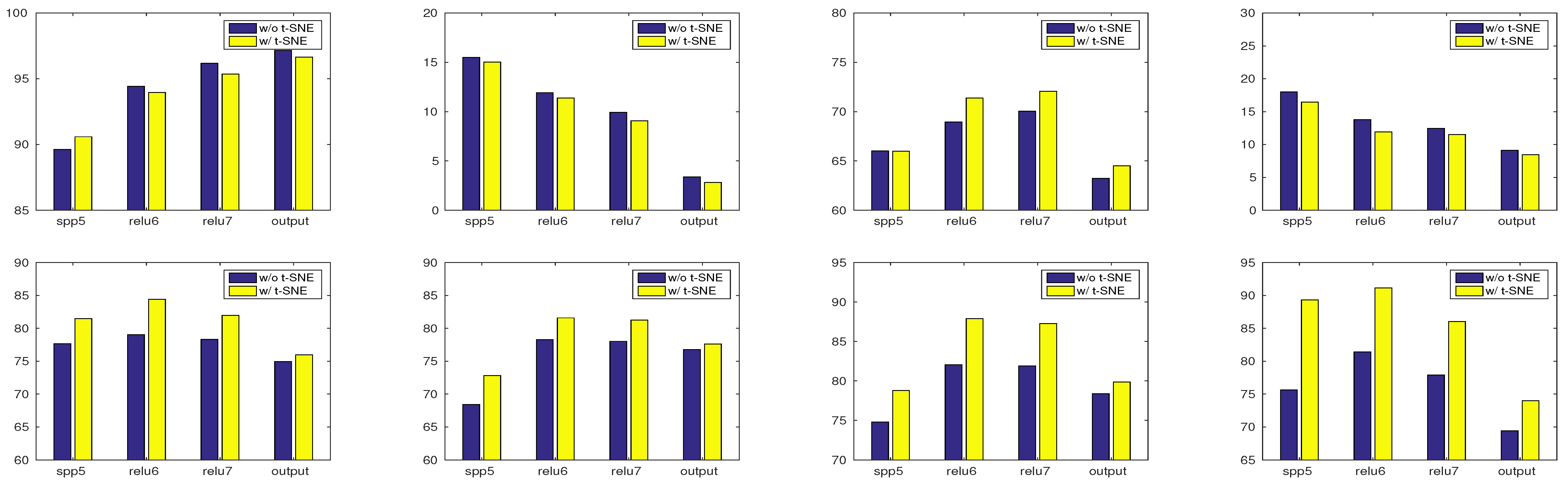
We have first trained our model on the IAM database, and run tests over itself (cross-validated folds) as well as GW20, Bentham14, Modern14. The parameters of the test were (a) extracting deep features from different network layers (we compare $spp5,relu6,relu7$) (b) applying t-SNE to produce low-dimensional embeddings or not (c) using different dissimilarity measures (we compare BC, L2, L2-normal). Prior to applying t-SNE, we first compute projections with PCA. As BC is suitable for use only with nonnegative vectors (preliminary tests of the BC on real-valued vectors have shown that performance deteriorates severely) we do not apply PCA in that case. The PCA projection and the t-SNE embedding dimension was fixed in all cases to 400 and 4 respectively.

A number of observations can be made on these results, presented in

Table 1. MAP results of KWS trials over different test sets, different layers to extract deep features, and different dissimilarity measures. PHOCnet trained on IAM was used in all cases. Figures are results obtained without using t-SNE embeddings.

	GW20
	BC	L2	L2-Normal
$spp5$	$\left(76.3\right)80.4$	$\left(74.9\right)78.4$	$\left(77.6\right)81.4$
$relu6$	$\left(82.1\right)84.1$	$\left(75.6\right)81.8$	$\left(79.0\right)\mathbf{84}.\mathbf{4}$
$relu7$	$\left(80.2\right)82.4$	$\left(74.7\right)79.5$	$\left(78.3\right)81.9$
output	$\left(76.0\right)78.4$	$\left(72.7\right)73.4$	$\left(74.9\right)75.9$
	IAM
	BC	L2	L2-Normal
$spp5$	$\left(59.5\right)63.6$	$\left(62.0\right)67.0$	$\left(68.4\right)72.8$
$relu6$	$\left(74.6\right)79.4$	$\left(70.0\right)75.6$	$\left(78.2\right)\mathbf{81}.\mathbf{5}$
$relu7$	$\left(75.5\right)80.0$	$\left(69.4\right)74.2$	$\left(78.03\right)81.2$
output	$\left(76.1\right)79.5$	$\left(73.5\right)74.4$	$\left(76.7\right)77.6$

. First, embedding with t-SNE gives in most cases a slight up to considerable boost. Concerning the best layer choice, deep features consistently outperform the “output” of the NN. Regarding the choice of dissimilarity measure, L2 gives the worst results. Both L2-normal and BC achieve improved results.

In Figure 1, we show a comparison of results using different layers to extract features. The L2-normal distance is used in all cases.

In

Table 2. Performance comparison (MAP%) of deep feature performance vs standard NN output. Results using models trained on IAM (a) and GW20 (b) are presented. The layers related to the best deep features are indicated, along with the boost compared to performance using standard NN output.

	(a)
	Deep Features	PHOCNet Output	Boost
GW20	$84.4\left(relu6\right)$	$75.9$	$+8.5$
IAM	$81.5\left(relu6\right)$	$77.6$	$+3.9$
Bentham14	$87.8\left(relu6\right)$	$79.8$	$+8$
Modern14	$91.1\left(relu6\right)$	$74.0$	$+17.1$
	(b)
	Deep Features	PHOCNet Output	Boost
GW20	$95.3\left(relu7\right)$	$96.6$	$-1.3$
IAM	$15.0\left(spp5\right)$	$2.8$	$+12.2$
Bentham14	$72.0\left(relu7\right)$	$64.5$	$+7.5$
Modern14	$16.4\left(spp5\right)$	$8.4$	$+8.0$

we present a list of the best performing deep features, and a comparison of their performance against extracting descriptors from the output layer. Note that in almost every case, deep features give the best performing descriptors. The difference between best layer and output in terms of MAP, can reach more than $17\%$ (Table 2, train on IAM/test on Modern14). A gain of 5–10% performance on average seems to be the norm. We report only results over t-SNE embedded features, which have shown slightly better performance as we have seen on the previous results; however they are strongly correlated to the results obtained without applying t-SNE. Only the output of the $GW20$-trained net seems to perform better than deep features, with a negative difference ($-1.3\%$). This can be explained due to the limited style variability of $GW20$, which leads to overfitted high results on itself and low results on other datasets. Bentham14 seems to be an exception, at least to a certain extent. This can be attributed to the similar style of these two datasets (for example, Almazán et al. [11] had trained a model on GW20 and tested it on Bentham14 with considerable success [13]).

Interestingly, deep features give improved performance even in cases when using the model output would give almost zero MAP (for example, Table 2, train on GW/test on IAM or Modern14). The case of training on GW20 is indeed particularly noteworthy: the same model gives figures close to $100\%$ when tested and trained on different folds of the same database, but results become very inadequate when tested on input coming from a different database. This is evidently a case of overfitting. In our opinion, this result is quite alarming, as many recent works have focused on obtaining the best figure with training and testing on the same database [1], neglecting to report how the same model would fare if tested on a different set.

On the other hand, deep features comparatively show better performance, even when using a model that has overfit on a specific set. This validates the point that deep features are transferable and lead to less specific, more general features compared to the network output.

Another interesting point is that features obtained from the NN trained on IAM are considerably transferable. We attribute this fact to the rich variability of the IAM dataset, which contains data coming from hundreds of writers, compared to the much smaller and less variable GW20 set. Furthermore, in this case, the t-SNE embedding achieves a noteworthy gain, regardless the layer or the dataset used. Deep features extracted using the NN trained on IAM, outperform all other methods in the literature compared on the sets of ICFHR’14 by a significant margin (

Table 3. Comparison versus state-of-the-art KWS methods. Results using the IAM-trained PHOCnet model are used to extract deep features.

Method	Bentham14	Modern14
Kovalchuk et al. [14]	$52.4$	$33.8$
Almazán et al. [11]	$51.3$	$52.3$
Howe [15]	$46.2$	$27.8$
Retsinas et al. [16]	$57.7$	$35.5$
Sfikas et al. [3]	$53.6$	$32.1$
PHOCNet output	$79.8$	$74.0$
Deep Features	$\mathbf{87}.\mathbf{8}$	$\mathbf{91}.\mathbf{1}$

).

4. Conclusions

In this work, we validate the usefulness of hidden layer activations for extracting deep features and use them to perform keyword spotting. With extensive numerical experiments, we have shown that these features are transferable; that is in the sense that their performance is by comparison more robust to being applied to different styles and sets. Such features achieve results significantly better compared to features obtained through the “standard” NN use, i.e., using its output.

We have also used different dissimilarity measures for descriptor comparison. Our results suggest that a form of normalization is beneficial for the task, regardless of the type of features. Concerning the Bray-Curtis dissimilarity in particular, we show that even if the motivation for its use was originally to compare histograms, it clearly works even for deep features, which do not have any such significance.

Also, the application of manifold learning led consistently to better results according to our experimental results. Compared with state-of-the-art methods applied on datasets of a recent KWS competition (Bentham14, Modern14) the proposed features lead to significantly superior numerical results, even though using a model trained on a different set (IAM).