1. Introduction
Transport systems play an essential role in the life quality and socioeconomic development of modern societies. Due to this relevance, four main issues of transport systems arise: travel safety, environment degradation, infrastructure sustainability and impact on the territory. The road-based transport is the most popular of the transport modes, especially in private transportation, and for this reason these issues have more relevance. According to the International Energy Agency, there were an estimated 900 million passenger light-duty vehicles on our roads worldwide in 2015, a figure that is projected to grow up to 2 billion by 2040 [
1]. The World Health Organization estimates that approximately 3 million people die every year due to health problems caused by pollution [
2]. A way to face these transport issues consists of efficient and safe road-based mass transit systems development that provide quality of service to the traveller.
The presented work is developed in the context of Intelligent Transport Systems (ITS) for road-based mass transit systems, and its aim is to obtain key data for the continuous improvement of these. Specifically, the purpose is the estimation, for each line service made by a vehicle of the fleet, the time spent traveling the scheduled path between each pair of consecutive stops on the route and the time when the vehicle is stopped at each stop of the route. From these estimations computed for each line service, the proposed methodology, based on Data Mining, obtain the behaviour patterns of these times. Using these patterns, reliable service scheduling can be made and develop measures to reduce the travel time or its variability of the public transport routes. It should be noted that the travel time is a key factor to provide quality of service, because the traveller wants to make his trips in the shortest time and with foreseeable travel times. This goal is coherent with the current paradigm of ITS, this is based on the continuous observation of what happen in the transport network and a feedback to improve the transport systems, user-based to solve the people mobility problem [
3]. To achieve this continuous observation of the transport network, the sensors systems and the data communication has a main role. In the proposed methodology, the positioning system, payment systems and mobile data communication used in the vehicles are key elements. In this point, the paradigm of cognitive transport network arises. In this particular one, the sensors installed in vehicles, infrastructures and user devices, acquire relevant data which is transmitted using different data communication technologies, recorded in the Transport Data Base (TDB) and processing using advanced techniques, such as Big Data or Data Mining, in order to obtain new knowledge to explain the behaviour of the transport network or to predict this behaviour.
The rest of this article is organized into five more sections. The second section lists works related to the proposed methodology. The methodology is described in the third section. Next, the results of a use case implementing the methodology in the study of the travel time of a bus line of a public transport company are presented. The fifth section is a discussion of the results, and the final section draws the conclusions.
2. Related Works
From the point of view of the activities required to develop efficient and safe mass transit systems, three are the main tasks involved: transport network design, service scheduling and monitoring and controlling of operations. A review of the methodologies used to make these tasks is presented in [
4]. In the context of road-based mass transit systems, the relationship between these tasks and service quality, describing the metrics used to evaluate it are described in [
5]. Information about the needs and habits of the people is a requirement to achieve the goals of these main tasks. Big Data and Data Mining provides useful techniques to obtain these information, arising the concept of cognitive transport networks [
6]. Next, a review of proposals which use Data Mining to evaluate and improve the quality of service of mass transit systems, or to know the traveller behaviour in the transport network is presented. First, proposals to improve to evaluate the quality of service, next proposals for forecasting the travel time and finally proposals to know the demand, habits and profiles of the transport user are.
The processing of vehicles positioning data by Data Mining techniques to improve mass transit systems is proposed in different works. Clustering techniques to analyse the impact of the traffic and the demand are presented in [
7]. The use of information on passengers boarding and alighting from vehicles to know how to avoid overcrowding in the transport network is proposed in [
8]. In practice, a bus driver may deliberately speed up or slow down on route to follow the predetermined timetable, in [
9] a methodology to calculate the real bus travel time is proposed. A new metric to evaluate the service punctuality is presented in [
10]. A model based on GPS monitored bus routes and association rules to improve the reliability of services scheduling is proposed in [
11]. The quality service evaluation using clustering techniques and ad-hoc metrics is proposed in [
12].
Works to predict the travel time (TT) based on vehicles positioning data processing by Data Mining are frequent in the bibliography. Neuronal networks are used in [
13,
14,
15] and classification techniques in [
16] and combining k-nearest neighbours regression are proposed in [
17]. The travel time forecast using k-means and v-means are presented in [
18]. In [
19] Kalman filters are proposed and time series in [
20]. Lastly, a hybrid model using Support Vector Machines and Kalman filters is proposed in [
21].
In relation with acquiring information about demand, habits or profiles of the transport user, a wide range of Data Mining studies have been conducted on these subjects. In [
22] a study about usage habits of the transport infrastructures is presented. How to make predictions about travel time, using data generated by payment systems based on contactless smart card, is described in [
23]. Also, using this same data source, in [
24] how to develop personalized information services for the transport user is presented. A proposal to obtain mobility pattern using also socio-demographic factors, such as location of shopping centers, sports areas, residential areas, etc., is presented in [
25]. The series of trips completed during certain time intervals and using statistical models is proposed in [
26] and using neural networks in [
27]. In [
28], the result of two different models of networks is analyzed using time-dependent parameters (trend, cycle and periodicity) in the observed demand data. Finally, a new hybrid optimization algorithm is developed in [
29], using set theory and neural network techniques, to predict the volume of passengers by road.
3. Methodology
In road-based mass transit system, TT and its prediction play a main role for providing quality of service. Firstly, because travellers want their journeys to last as little as possible. Secondly, because they expect punctuality. To satisfy these travellers expectative, knowledge about the TT behaviour of public transport journeys is required. The challenge is that TT, in road transport, is affected by factors of very different nature: traffic conditions, demand, weather, etc.
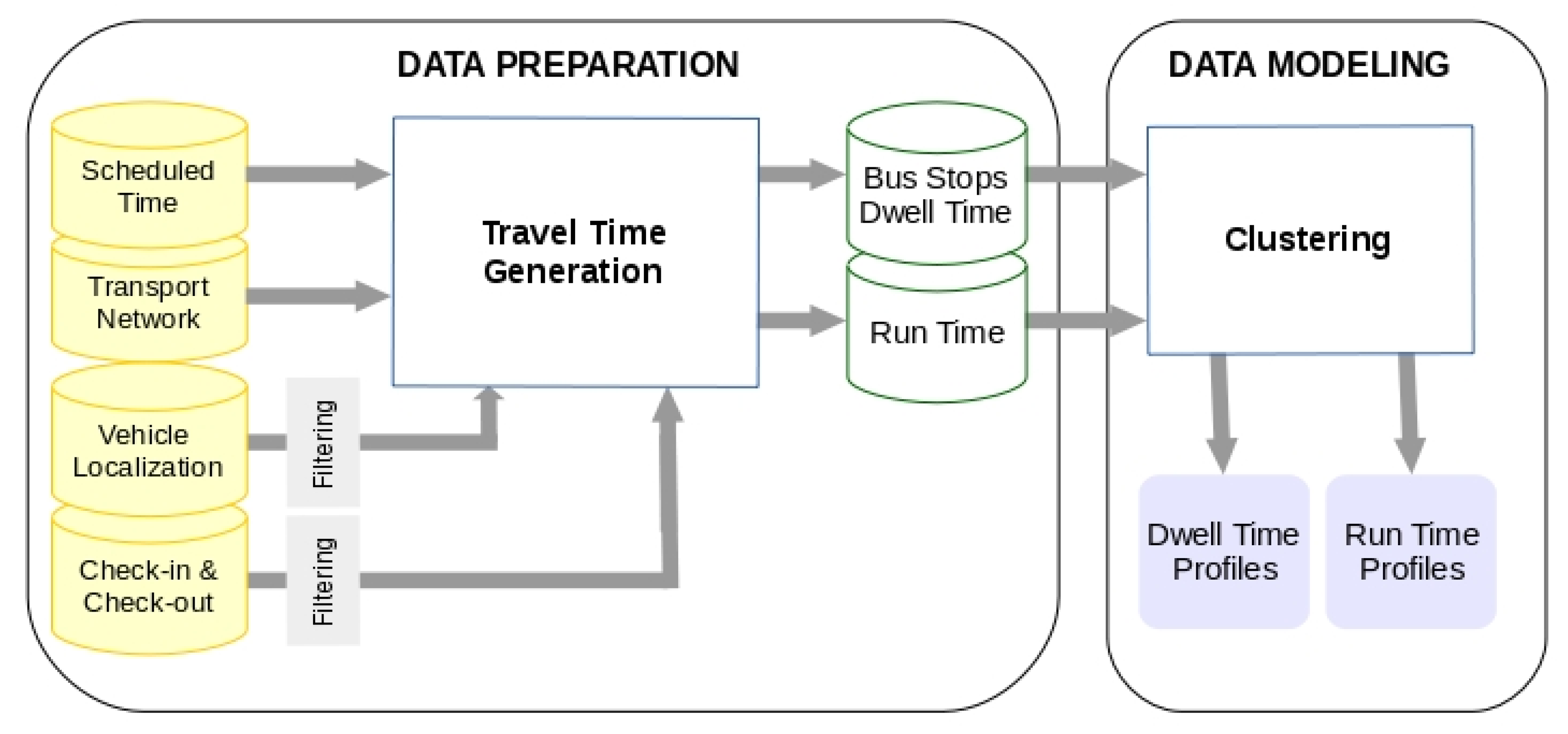
The methodology proposed in this paper has two goals. Firstly, to obtain systematically the two times components of the TT of a route made by a public transport vehicle: the nonstop running time in the road segment between each pair of two consecutive bus stops (RT) and the dwell time at each stop (DW). Secondly, obtaining these time for each vehicle journey of a line, it is possible to generate the patterns of these times and next to identify the factors which affect to TT.
To achieve the first goal, the methodology uses the data provided two systems installed on vehicles: the payment systems, based on contactless smart card, and the positioning system based on GPS. These data are obtained from de data records generated in each line service made by the vehicles of the public transport fleet. Therefore, the deployment of specific technological infrastructure is not required to obtain these data. To achieve the second aim, the RT and DW data are processed using machine learning techniques to understand the TT behaviour based on patterns of RT and DW. The proposed methodology permits systematically to reach these goals mined data records obtained from TDB.
Figure 1 shows the proposed methodology.
3.1. Formalization
A requirement of the proposed methodology consists of generality, assuming generality as the capacity to be applied in different types of road-based mass transit systems. To fulfill this requirement, all the entities used are contemplated in international standard specifications about conceptual data models for transit systems [
30].
The first entity to formalize is the public transport network. This can be represented by graph G, G = (N, A). N represents the set of nodes of the network, N = {ni}. Each node, ni, represents a relevant point for public transport activity, such as: bus stops, stations, time control points, garages, etc. For the presented methodology, nodes represent bus stops. A is the set of arcs which connect to nodes of the set N. The arcs represent routes taken by vehicles and travelers. For the methodology porpoise, the significative arcs are the used to define the routes pathed by the vehicles transporting travelers. The next concept to formalize is the route pathed by a public transport vehicle transporting travelers, this is represented by ri. Each route ri is defined as the path followed by the vehicles, and comprises an ordered sequence of arcs. If route ri has n arcs, then ri is specified by n-tuple (ai, …, an). From the route entity, the line entity is defined as a set of very similar routes from the topological point of view (usually a round trip) represented by li. The set of lines in the transport network is represented by L, L = {li}.
The next entities to formalize are related to service scheduling. The service scheduling to make in the transport network is represented by the set S, S = {si}. Each si represent a scheduling unit, and it is defined as an ordered of transport operations which must be made by a vehicle during a period. For the porpoise of the methodology, the transport operations to consider are the line services to make in the scheduling units. Each of the completed operations of a line service made by a vehicle is called a Vehicle Journey, represented by VJ. The VJ set of all the routes of a line L is represented by {VJ}L, to express the VJ set of a line L completed in a period of time T the notation {VJ}L,T is used.
Formally, for a VJ of route
r, if the route has Ns bus stops and Na arcs, TT is expressed as follows:
DWn represents the dwell time at bus stop n and RTn is the nonstop running time of the arc n.
3.2. Data Preparation
The goal of this phase is to build a data set suitable to execute the Artificial Intelligence (AI) techniques used in the proposed methodology. This data set is generated from the data records of the TDB. All the relevant entities for representing the transport activity is recorded in this database. For the aims of the methodology, the data records representing the relevant events produced during the vehicles services are the source data to consider. More specifically, the event records processed in this phase are:
Passenger Check-in (PCIR). This record represents a passenger check-in recorded by a payment system based on contactless smart card installed on the vehicles. This record contains data fields specifying the check-in operation that are: time, expressed in Universal Time Coordinates (UTC), indicating when the check-in was made and line and bus stops indicating where the check-in was made.
Passenger Check-out (PCOR). This record represents a passenger check-out recorded by a payment system based on contactless smart card installed on the vehicles. This record contains data fields specifying the check-out operation that are: UTC time to represent when the check-in was made and line and bus stops to represent where the check-out was made.
Vehicle Positioning (VPR). This record represents the vehicle position recorded by positioning system based on GPS installed on the vehicles. This record contains data fields representing a GPS reading, that are: latitude, longitude, Altitude, velocity, UTC time when the GPS reading was acquired and reading quality.
To guarantee the reliability of the results, a basic goal to achieve in this phase is the data integrity. For this reason, all the data records representing these events are processed to detect records containing incorrect data fields, such as incoherent times, non-valid lines or bus stops. Additionally, only data records obtained in vehicle journeys which have pathed a complete and coherent route is selected for the AI processing. In this case, coherent and complete route means that the vehicle has pathed all the arcs of the route. All the processes executed to make these verifications with the TDB data records are grouped in a sub-phase called Pre-processing.
The input specifications of this phase are the line (L) and the period (T) to analyze. From these input data, the data records representing the mentioned events produced in the vehicles when these made the line L during the period T, are retrieved from TDB. Following, the Pre-processing is executed. The output of the Pre-processing is a set of data records obtained at complete and coherent vehicle journeys of the Line L during T, this data records set is named {QDRS}L,T and the set of complete and coherent vehicles journeys is called {QVJS}L,T.
The last step in the Data Preparation Phase is to obtain the DW and RT for each vehicle journey belonging to {QVJS}L,T. These sets of times are named {DW}L,T and {RT}L,T. These are deduced from the {QDRS}L,T records. The estimation of these times for each vehicles journey is made considering the time of the check-in and check-out operations recorded at each bus stop of the journey, being the DW the difference between the maximum value and minimal value of these times. If at a bus stop there are not check-in and check-out operations registered, this time is zero. The RT value of an arc joining two consecutive bus stops, s0 and s1, is estimated as the difference between minimal time of the check-in or check-out operations at s1 and the maximum time of check-in or check out operations at bus stop s0. If at one of the bus stops no check-in and check-out operations were produced, then the time at that bus stop to calculate the RT is the pass time which is estimated using the VPR records acquired during vehicle journey.
In this point, the datasets {DW}
L,T and {RT}
L,T. to be used by AI techniques is generated. These datasets are formed by a set of data records in which each record is related to a VJ belonging to {QVJS}
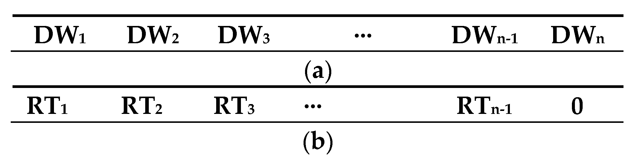
L,T, containing the DW and RT times of the VJ. The structure of the records of these sets for a line with
n bus stops is showed in
Figure 2. In
Figure 2a,
DWn represents the dwell time at the bus stop
n. In
Figure 2b,
RTn represents nonstop run time of the arc
n.
3.3. Modelling
The goal of this phase is to obtain the behaviour patterns of the RT and DW of the studied line. As these patterns depend on temporal, space and demand attributes, such as period of the year, week day, time of day, type of road, etc., an additional goal is to explain these patterns basing on these attributes.
The AI used to obtain the behavior patterns are clustering techniques. These techniques are capable of handling large datasets and are frequently used in transport Data Mining projects. More specifically, the k-Medoid clustering is the technique used [
31], because this is more robust against noise that other classic clustering techniques such as K-means. In k-Medoid method, the centroid, named medoid, is an element of the cluster whose average dissimilarity to all the elements of the cluster is minimal. With the other elements of the group. To evaluate the quality of the clustering solutions, the Silhouette function is used. This function measures the consistency of the clusters generated, based on the separation and tightness of the elements of each cluster by the expression represented in Formula (2).
In Formula (2), a(i) is the average distance from element i to other elements within the cluster, and b(i) is the smallest average distance from i to all the elements of each of the cluster to which i does not belong. The k-Medoid clustering is applied to datasets {DW}L,T and {RT}L,T.
4. Results
The results reached to apply the proposed methodology are presented in this section. The case of use consists of analysis the TT of a line of a company of public transport by the proposed methodology using the data provided by the company. The TT behaviour of the line has been studied during all the year 2015, so in the proposed formalization the period T is the year 2015, that is T = 2015.
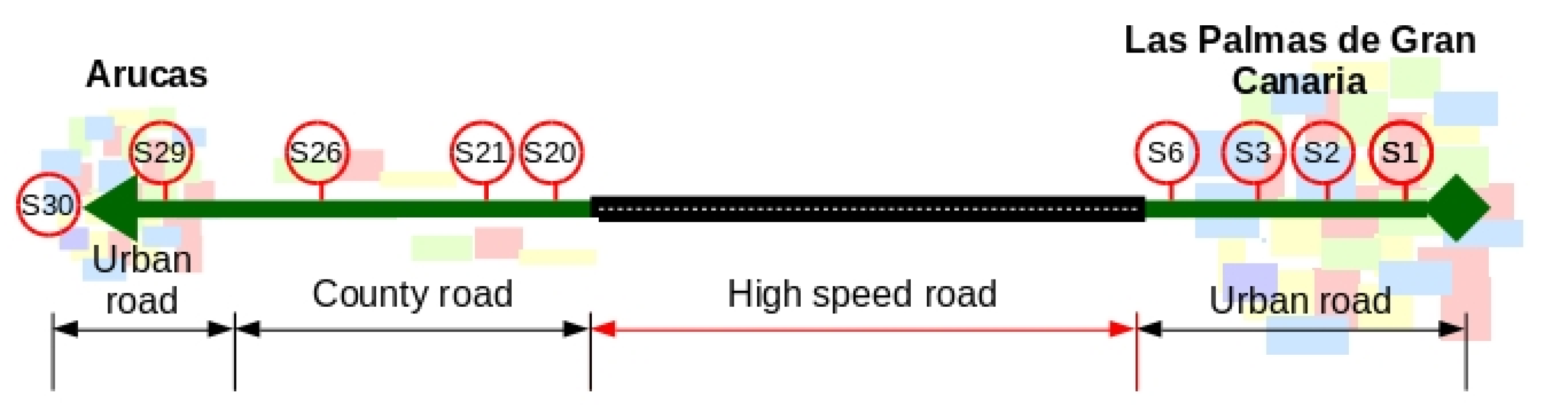
The studied line is identified by transport operator using the code 210. Therefore, in the proposed formalization the variable L adopts the value 201, that is L = 2010. The route of the line has 30 bus stops, covering 23 km, departing of an urban area and ending in other urban area. The route is formed by three sections: the first paths an urban area, the second is across a non-urban area using a highspeed road and a country road, and the third paths other urban area.
Figure 3 shows a schematic representation of the line. In this representation, only the ten most used bus stops of the line are drawn and the cities crossed; starting at Las Palmas de Gran Canaria and ending at Arucas, both cities are in Gran Canaria island (Canary Islands, Spain).
About the scheduled line services, during the studied period that is the year 2015, the vehicles journeys were made using two scheduling: one of them for Mondays to Fridays excluding public holidays, and other for Saturdays, Sundays and public holidays. In the scheduling for Mondays to Fridays excluding public holiday, the first vehicle journey starts at 06:30, the next vehicles journeys start from 07:10 to 20:40 every 30 min, and the last two vehicle journeys start at 21:30 and 22:15. In the scheduling for Saturdays, Sundays and public holidays, there are fifteen vehicle journeys scheduled, the first thirteen are scheduled from 08:40 every 60 min, and last two at 21:30 and 22:15.
Table 1 shows the planned arrival times for each of the 30 stops on the route. The first stop, stop 0, is not included in
Table 1 since it is assumed that the vehicle starts the VJ at the scheduled time. Each stop on the line has been identified in the order of arrival following the set route; the stops correspond to the labelled points 0 to 16 and 18 to 30.
About the passengers which used this line in 2015,
Table 2 shows the use of each bus stop by the passengers of the line. This data has been obtained using the check-in and check-out records.
In the data preparation phase, Oracle was used for the database system and Pentaho for integration and visualization.
In the modelling phase, the RStudio framework was used; more specifically, the PAM function of the Cluster package [
32], selecting the Euclidean distance as the metric for calculating the dissimilarities between the data and without determining the initial medoids.
4.1. Data Preparation
The goal of this phase is to obtain the {DW}
210,2015 and {RT}
210,2015, Applying the concepts and techniques of the Data Preparation Phase explained in the previous section. The first step consists of obtaining, from TDB, all the vehicle journeys of the line 210 during the year 2015, that is {VJ}
210,2015. From the services scheduling of the year 2015, the number of vehicles journeys would be 9675. The next step is the subset of {VJ}
210,2015 formed by coherent and complete vehicle journeys, that is {QVJ}
210,2015. Following the methodology explained in the previous section, the number of vehicle journeys of {QVJ}
210,2015 was of 7654. The reason of this difference, between theoretical number of scheduled vehicle journeys and the number of complete and coherent vehicle journeys registered in the TDB, could be due to data lost as consequence of device or data transmission faults. In
Figure 4, the vehicles journeys of the line 210 during the year 2015 are represented. The red curve represents the theoretical number of vehicle journeys of each scheduling expedition and the vertical lines represent the complete and coherent vehicle journeys recovered from the TDB. The scheduled vehicle journeys are represented in the horizontal axis. The vehicle journeys identifiers between 1 and 31 correspond to vehicle journeys scheduled for Mondays to Friday (excluding public holidays). The vehicle journeys identifiers from 32 onwards correspond to vehicles journeys scheduled in Saturdays, Sundays and public holidays. The number of vehicle journeys processed is represented in the vertical axis.
The last step in this phase of the methodology consists on estimating the dwell times and non-stop run times at each bus stop for each vehicle journey of {QVJ}210,2015 dataset, that is {DW}210,2015 and {RT}210,2015 datasets. Using the methodology explained in the previous section for estimating these times, the number of DW obtained was of 5893 and for RT was 5741.
4.2. Modelling
From the dwell and no-stop sun time datasets, {DW}
210,2015 and {RT}
210,2015, the goal of this phase is to know the behaviour patterns of these times. Specifically, the aim is to understand how certain time-dependent factors, such as the type of calendar day and the time of day, affect the behavior of these times. To this end, the k-Medoid clustering technique was applied to {DW}
210,2015 and {RT}
210,2015 datasets. The clustering technique was executed using three clusters.
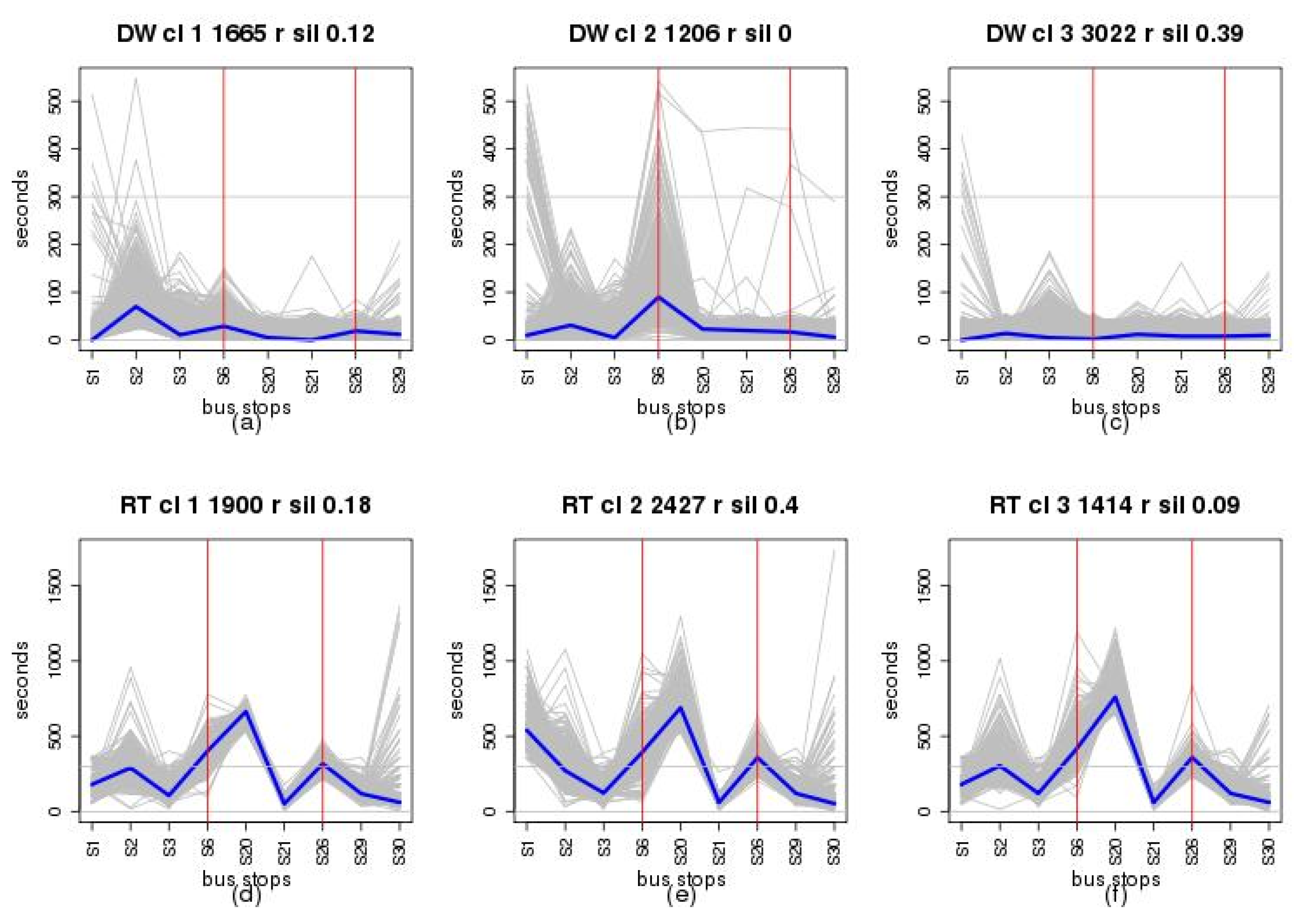
Figure 5a–c show the results for {DW}
210,2015 and
Figure 5d–f show the results for {RT}
210,2015. To facilitate the graphic visualization in these figures, the ten most used bus stops of the analysed line are represented. These bus stops are 0, 1, 2, 3, 6, 20, 21, 26, 29 and 30. In the figures, the vertical axis represents the times (DW or RT), and the horizontal axis the stops analyzed. The three red vertical lines represent the three sections into which the route was initially divided: urban, intercity, and urban section. In each graph, the blue line represents the medoid of each resulting cluster group, and gray lines represents the elements classified in each cluster group. The elements number and the cohesion value computed by Silhouette function are presented in the top part of each graphic.
In the case of {DW}
210,2015 clustering, the cohesion values for each of the clusters were 0.12 (Cluster 1), 0.00 (Cluster 2), and 0.39 (Cluster 3). About the number of vehicle journeys of each cluster, these are: 1665 (Cluster 1), 1206 (Cluster 2) and 3022 (Cluster 3). See
Figure 5a–c.
For the {RT}
210,2015 clustering, the cohesion values for each of the clusters were 0.18 (Cluster 1), 0.4 (Cluster 2), and 0.09 (Cluster 3). About the number of vehicle journeys of each cluster, these are: 1900 (Cluster 1), 2427 (Cluster 2) and 1414 (Cluster 3). See
Figure 5d–f.
5. Discussion
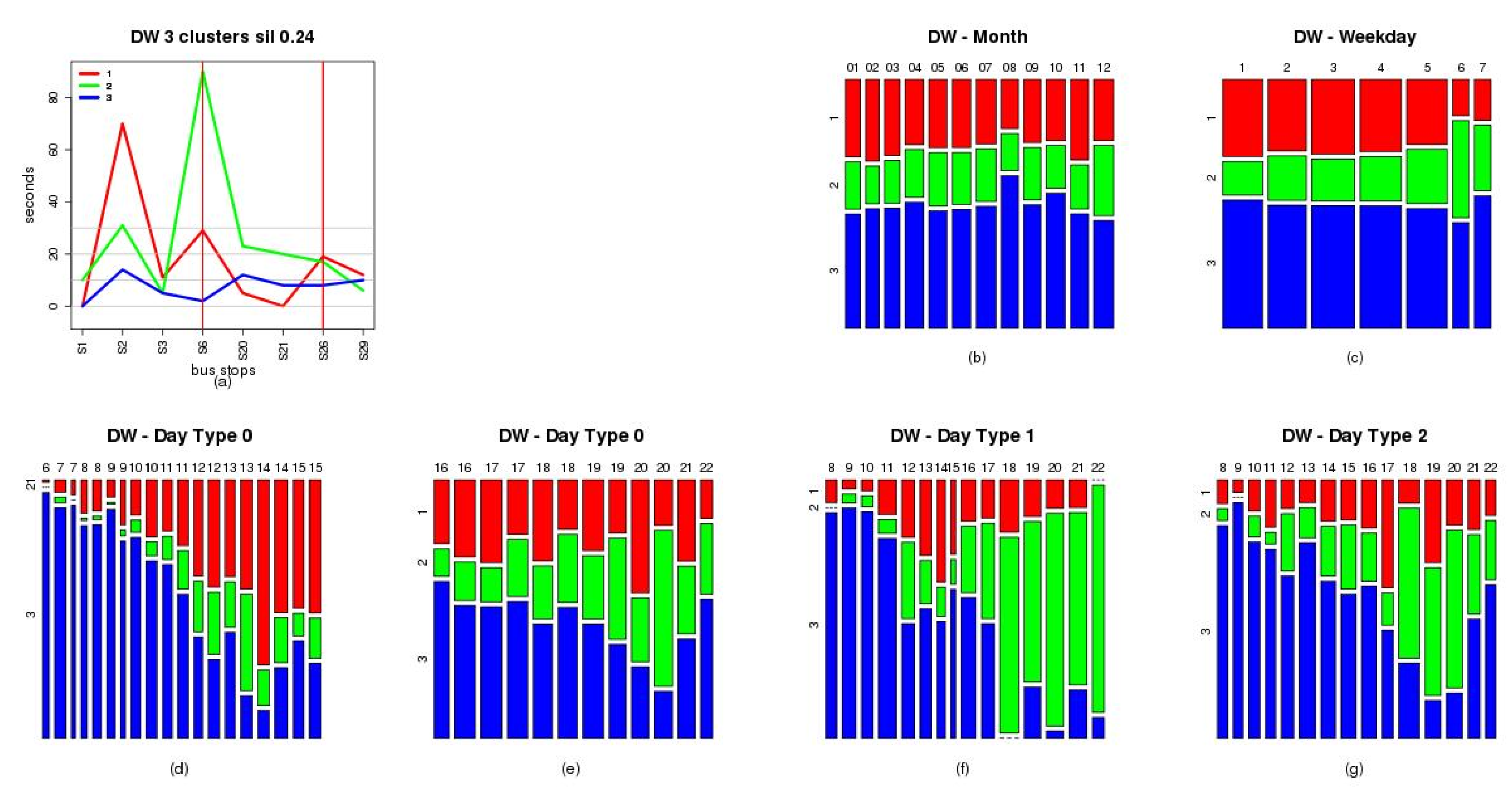
From the results obtained in the analysis of DW, it may conclude that the behaviour of this time follows three different patterns. In the first, the major dwell is produced at the bus stop number 2 of the line, being the value of the medoid for this bus stop about 80 s. In the second pattern, the major DW is produced at the bus stop number 6, being the value of the medoid for this bus stop about 100 s. In the third pattern, the behaviour of the DW is very similar during the vehicle journeys belonging to this cluster, being the values of the medoid in every bus stop very close to zero. This last pattern could be corresponded to vehicle journeys with very low demand. To explain these behaviors of the DW, two facts must be considered. The first is that the main travel generator source in the transport network studied is the city of Las Palmas de Gran Canaria, crossing the first segment route (from the first bust stop to seventh bus stops of the line) this city. The second to be considered is that the sixth bus stop of the line is located I a shopping and leisure area. These facts could explain the number of users of each bus stop and the values of DW. The four bus stops most used are the first, third, seventh and last.
Combining the results obtained in the analysis of the DW and RT at stops, it may be concluded that major contribution of these times to the TT is dues to RT. More specifically, the magnitude of TT is mainly influenced by RT and the TT variability is principally affected by the segment of the route from first bus stop to the bus stops number 3.
Figure 6a the medoids of each DW pattern is showed.
Figure 6b shows the contingency table relating patterns frequency with the month of the year, observing very similar values in all the months. Also, the pattern associated to a low demand, pattern 3, is the most frequent in the month of August which is a typical holiday period.
Figure 6c shows the relationship between patterns frequency with the day of the week. Observing this figure, it can be concluded that from Mondays to Fridays the patterns frequencies are very similar, but in Saturdays and Mondays the pattern 2, representing that the most used bus stops of the line is the seventh located in a shopping and leisure area, is the most frequent. In
Figure 6d–e the contingency tables representing the relationship between patterns frequency and scheduled departure hour of the vehicles journeys are showed. Observing these figures, it can conclude that the pattern associated to a low demand, pattern 3, is the most frequent from 06 to 11 h of the morning. The pattern 1, associated to a major use of the firsts bus stops of the line, is the most frequent from 14 to 15 h of the day. These results reflect that the line is used by the passenger as a return line when the service and labour activities end.
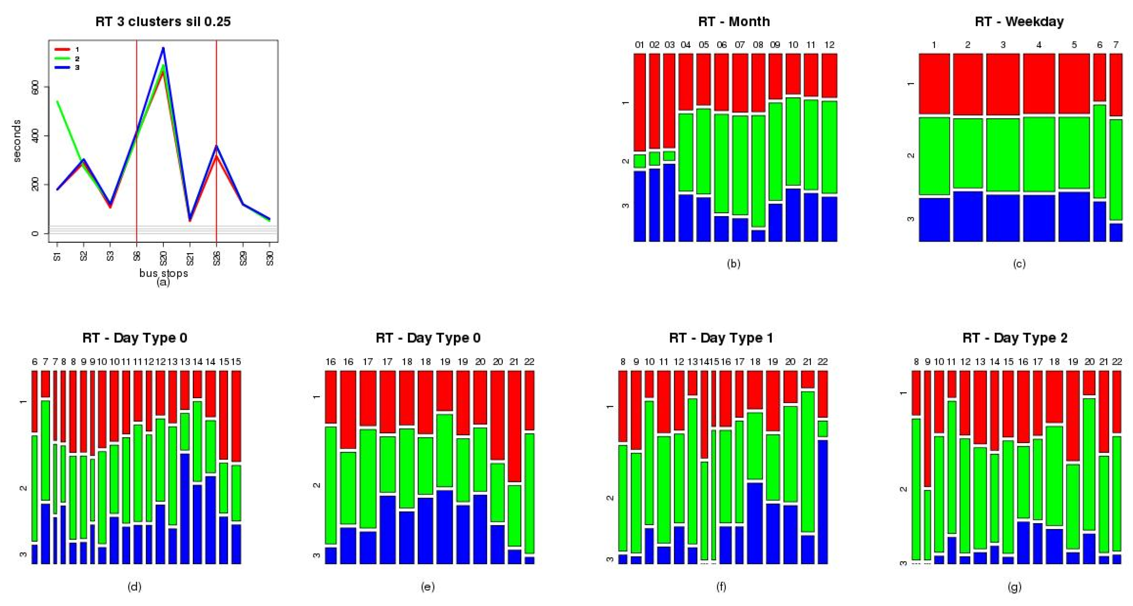
From the results obtained in the analysis of RT, it may be concluded that the behaviour of RT is very similar from bus stop number 3 to the end of the line, but different from the first bus stop to the bus stop number 3. This behaviour could be motivated by two causes. The first could be that segment of the route from first bus stop to the bus stop number 3 cross an urban are with very dense traffic at peak hours. The other possibility is that a significative number of vehicles journeys departures are delayed. As in the case of DW, using contingency tables to relate the frequency of each pattern with the temporal attributes.
Figure 7a shows the medoids of each cluster.
Figure 7b–c shows two contingency tables relating to patterns frequency with month and week day respectively.
Figure 7d–e shows the contingency tables relating to patterns frequency with the scheduled departure hour of each vehicle journey in labour days (Mondays to Fridays). In these tables, the pattern two is the most frequent at hours which are not peak hours. The table showed in
Figure 7f relates to patterns frequency with the scheduled departure hours in Saturdays. In this table, the pattern two is the most frequent at any departure hour. The last table,
Figure 7g, shows the relationship between patterns frequency and scheduled departure hours in Sundays or public holidays. Also, this table shows that the pattern two is the most frequent for any departure hour. Because of these results, the conclusion is that this behaviour of RT is motivated by the second cause.
Relating to the frequencies of each three patterns of DW with the month, week day and scheduled departure hour of each vehicle journey, it may conclude that the explanation about the pattern behaviour is correct.
6. Conclusions
To provide quality of service in mass transit systems it is necessary to reach high level of reliability in the services scheduling. In the context of road-based mass transit systems, due to the variability of different factors which affect to the transport activity, to achieve this goal is a challenge. In this kind of systems, to understand the behavior of the TT is a key factor to develop reliable services scheduling. In this work, a novel methodology, based on Data Mining, to known and understand the behavior of TT based on DW and RT has been presented. To reach this goal, the methodology uses data representing vehicles positioning and check-in and check-out movements of the passenger. By these data, it enables the DW and RT of the different scheduled routes to be systematically analyzed, guaranteeing the validity of the results by subjecting the data to validation processes. In addition, to reach a high level of generality for road-based mass transit systems, standard data models and metrics have been assumed by the proposed methodology. To obtain the behaviour patterns of DW and RT, the k-Medoid-based clustering technique is used. By this clustering method, these patterns are generated in order to know what factors affects to TT and its variability and this way, to deploy measures to reduce the TT or its variability. The methodology has been applied to a real case, consisting of analysing the DW and RT of a line of public transport. The results obtained demonstrate the validity of the proposed methodology.

 ,
, 


