Abstract
Pumps As Turbines (PATs) can be installed in Water Distribution Networks (WDNs) to couple pressure regulation and small-scale hydropower generation. The selection of PATs in WDNs needs proper knowledge about both the performances of machines available in the market and the operating conditions of the network. In this paper, a procedure for the preliminary selection of a PAT is proposed, based on the design of the main parameters (the head drop and the produced power at the Best Efficiency Point, the impeller diameter and the rotational speed) to both maximize the producible power and regulate the exceeding pressure.
1. Introduction
In the last years, the use of micro-turbines and/or Pumps As Turbines (PATs) in Water Distribution Networks (WDNs), instead of Pressure Reducing Valves (PRVs), is attracting significant attention, because they allow both pressure regulation and small-scale hydropower generation.
The installation of PATs is an effective alternative to micro-turbines, since can combine high efficiency, low investment and maintenance costs, ease of installation and spare-parts procurement [1]. Conversely, one of the main issues arising from the use of PATs for power generation is the lack of knowledge about their characteristic curves, only rarely provided by manufactures.
In the literature, several models were proposed to predict the PAT performances; many of them were devoted to predict the characteristics at the Best Efficiency Point (BEP), as a function of the performances at BEP in pump mode, through one-dimensional formulations, as summarized in [2]. The Affinity Laws [3] are widely applied to reproduce the performances of turbo-machines operating in similitude, as well. However, their reliability results not highly effective for several pump models running as turbines, such as semi-axial and submersible models [4]. Further approaches were devoted to predict the characteristic curves of PATs by means of laboratory experiments. Among them, Derakhshan and Nourbakhsh [5] proposed second-order and third-order polynomial equations to estimate the head drop curve and the power curve, respectively for single-stage horizontal axis centrifugal PATs. In both cases, equations were given in dimensionless terms with respect to the BEP. The reliability of such curves was limited to specific speeds in direct operation Nsp up to 60 and flow rate numbers φ up to 0.40, where:
with N the rotational speed (rps), Q the flow rate (m3/s), H the head (m) and D the impeller diameter (m). The subscript p refers to the pump mode.
By means of laboratory experiments, Pugliese et al. [2] showed the reliability of the head curve given in [5] for flow numbers up to 1.30 for both horizontal and vertical axis centrifugal PATs. Conversely, the power curve is unreliable for flow numbers greater than 0.40, thus the authors provided alternative formulations, valid again for φ up to 1.30. They also proposed alternative formulations to predict the characteristic curves of both single-stage and multi-stage vertical axis PATs [6]. Stefanizzi et al. [7] developed a predictive model of single-stage centrifugal PATs model to estimate both the flow rate and the head ratios, as a function of the specific speed in direct mode Ns. Barbarelli et al. [8] implemented a recursive procedure to predict both the flow rate and head ratios and the characteristic curves of centrifugal PATs.
Despite the contributions available in the literature, the optimal selection of a PAT in WDNs is still a complex issue, due to the variable operating conditions of the system. Fontana et al. [9] applied a genetic algorithm to assess the energy recoverable by PATs in a district of the Naples (IT) WDN, observing attractive profits and short capital payback periods. Similar approach was considered by [10], aimed at installing PATs in the WDN proposed by [11]. In [12], the PAT reliability in the Kozani (GR) Municipality was tested, as a complementary practice to the District Metered Areas (DMAs) sectorization, resulting the application effective when the energy consumption was nearby the energy recovery site. Venturini et al. [13] analyzed the influence of the PAT application and selection in WDNs, whereas Fecarotta and McNabola [14] tested the effectiveness of an original optimization model to a benchmark WDN, aimed at maximizing both the energy production and the economic savings related to the leakage reduction.
Moreover, for the effective PATs regulation in WDNs, the activation of Hydraulic Regulation (HR) and/or Electrical Regulation (ER) could be considered, to extend their flexibility to the variable hydraulic conditions of the network. In [15] the Variable Operative Strategy (VOS) was proposed to provide the optimal selection of a PAT in WDNs, among a set of available models, able to maximize the overall plant efficiency, under the hypothesis of HR. The VOS was also applied to the case of ER [16], as well. Nevertheless, models available in the literature are mainly based on the use of either huge time-consuming simulation models or recursive and trial-and-errors procedures, in some cases requiring specific setting parameters referring to geometric and technical properties of the selected PAT model.
Aimed at design the main characteristic parameters for the optimal PAT selection in WDNs, in this paper a simple and effective procedure is proposed, to both maximize the producible power and energy and perform the pressure regulation, in compliance with the hydraulic and technical constraints of the system.
2. Materials and Methods
A procedure for the optimal selection of centrifugal PATs in WDNs is proposed, aimed at the design of the PAT characteristic parameters, namely the flow rate and the head drop at BEP Qtb and Htb (where the subscripts t and b refer to the turbine mode and the BEP, respectively), the impeller diameter D and the rotational speed N. The model was developed under the hypothesis of performing the ER by varying the electrical frequency f (Hz), so as to modulate the PAT rotational speed N at any operation in the range [Nmin; Nmax].
The first step allows to design Qtb and Htb, as a function of the maximum flow rate Qt,max. To both maximize the producible power Pt,max and exploit the whole available head drop Ht,av_max, second and third order polynomial functions are applied to reproduce the Ht(Qt) and Pt(Qt) curves, respectively, in compliance with [2,5]. Experimental data from [2] are considered, by refining the parameters estimation for φ ≤ 0.30, aimed at improving the interpolation around the BEP, which was found at φ = 0.18 from experiments. Equation (3) is derived to represent the Ht curve, setting the equivalence between the head drop Ht and the available head Ht,av_max when Qt,max flows:
The power curve from [2] is also considered to calculate the produced power Pt,max for Qt,max:
The power at BEP Ptb in Equation (4) can be calculated as:
where ηtb (-) is the PAT efficiency at BEP and γ (N/m3) the fluid specific weight. Expressing Htb by means of Equation (3), from Equation (4) it follows:
The maximum produced power Pt,max at varying Qt,max/Qtb is estimated as:
Once calculated Qtb from Equation (7), Equation (3) can be used to calculate the head drop at BEP Htb. From Equation (7) it is observed that the power maximization is achieved at flow rate ratios Qt,max/Qtb close to 1. Thus, from Equation (3) to optimize the exploitation of the available head, the head at BEP Htb should be approximately equal to Ht,av_max.
The specific speed in turbine mode Nst and the specific diameter Dst are set equal to 29.39 and 2.52, respectively in order to design machines with efficiency ηtb of the order of 80% [17]:
By combining Equations (8) and (9), the flow rate number at BEP φb can be derived, according to the following Equation (10):
By applying an optimization procedure validated with numerical and laboratory experiments, Fontana et al. [18] observed that the maximum producible energy can be achieved by setting φ = 0.185, corresponding to Qt,max/Qtb ratio equal to 1.450.
From Equations (8) and (9), the rotational speed N and the impeller diameter D able to both maximize Pt,max and exploit the available head Ht,av_max can be calculated, as a function of Qt,max.
Finally, by applying one of the one-dimensional flow rate and head ratios models available in the literature (e.g., the Yang et al. [19]), the flow rate and the head at BEP in pump mode Qpb and Hpb can be assessed, so as to identify the most effective PAT, among those commercially available, with impeller diameter D.
In case Pt,max achieves a value of N higher than the upper limit Nmax, then Nmax can be set to design the impeller diameter D. In this case, as a function of the flow rate Qt,max and the available head Ht,av_max, it is possible to choose whether:
- to maximize the producible power Pt,max, by calculating Htb from Equation (8) as a function of Qtb derived from Equation (7);
- to exploit the available head (e.g., Ht,exp = Ht,av_max), by calculating Qtb and Htb from Equations (3) and (8) and then the producible power Pt,max with Equation (4).
After the PAT has been selected, the operation in the other conditions should be analysed, e.g., in case of daily demand pattern for a WDN. At any flow rate, N can vary in the range [Nmin; Nmax], choosing either to exploit the whole available head Ht,av or to maximize the produced power Pt. The value of N able to maximize Pt in Equation (4) is calculated, by combining Equations (2) and (11). Equation (12) expresses Ptb as a function of the power number πb at the BEP:
where ρ (kg/m3) is the fluid density, resulting:
The flow rate number φb and the head number ψb at BEP can be also calculated using Equation (2) and the following Equation (13), respectively:
with g (m/s2) the acceleration of gravity. Being φb, ψb and πb constant at varying the rotational speed N [2], their calculation is useful to estimate the flow rate Qtb, the head drop Htb and the power Ptb at BEP at different N, respectively.
By applying the proposed procedure, the main parameters of PATs can be designed, so as to assess the overall producible energy and the corresponding payback periods.
Similar approach can also be applied to WDNs without ER, in which the PAT runs at constant rotational speed. In this latter case, Equations (3) and (7) can be applied either to exploit the available head drop or to maximize the produced power, respectively.
3. Results and Discussions
The procedure proposed above was applied to a WDN serving 20,000 inhabitants, with average flow rate Qtm = 57.9 L/s and maximum flow rate Qt,max = 83.3 L/s. The daily demand pattern provided by [9] and plotted in Figure 1 was considered. Two Scenarios were simulated, at varying the available head as summarized in Table 1. A horizontal centrifugal PAT was assumed in the example. For any scenario, a value of 0.5 kW was set as the minimum produced power. For lower produced power, the exploitation of the head drop Ht,av was assumed.
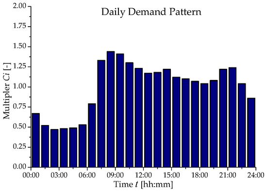
Figure 1.
Daily demand pattern for two considered Scenarios.

Table 1.
PAT design parameters as a function of Qt,max/Qtb ratio—Scenario 1.
For both Scenarios, the maximum flow rate Qtmax was equal to 83.3 L/s, whereas the available head Ht,av at Qt,max was 18.30 m for Scenario 1 and 88.30 m for Scenario 2. In Scenario 1, the procedure was applied as per following steps, by first setting Qtmax/Qtb = 0.951 (Equation (7)) and then Qtmax/Qtb = 1.450 to maximize the produced power and the daily producible energy, respectively. Qt,max was achieved at 08:00.
- Power Maximization at Qtmax: Qtmax/Qtb = 0.951
From Equation (7) the flow rate at BEP Qtb = 87.6 L/s was estimated as a function of Qt,max. The head drop at BEP Htb = 19.7 m was calculated with Equation (3). By setting Nst = 29.39 (Equation (8)) and Dst = 2.52 (Equation (9)), the rotational speed N = 15.5 rps and the impeller diameter D = 0.354 m were derived, respectively. According to Equation (10), the flow rate number at BEP φb = 0.128 and the power at BEP Ptb = 13.6 kW was estimated by Equation (5) as a function of the efficiency at BEP ηtb = 0.80. By applying the Equation (4), a maximum produced power at Qt,max Pt,max = 12.0 kW was thus obtained. Being N < Nmax (set equal to 50 rps) for further time-steps, the rotational speed N which maximized the producible power was derived by using Equation (12). N was assessed in the range from 7.5 to 19.5 rps. From Equations (11) and (13), the power number πb and the head number ψb at BEP were defined equal to 6.44 and 0.66, respectively.
Being φb, πb and ψb constant at varying N, from Equations (2), (11) and (13) the flow rate at BEP Qtb, the power at BEP Ptb and the head drop at BEP Htb were calculated, respectively, at any hourly time-step, as a function of the flowing rate Qt and the corresponding N. From Equation (3) Ht,exp was estimated at any time-step. For time-steps with Ht,exp > Ht,av the rotational speed N which set the equivalence Ht,exp = Ht,av was thus applied. Finally, with Equation (4) the produced power Pt was assessed at any hourly time-step and the corresponding PAT efficiency ηtb was estimated with Equation (5), resulting in the range 68 ÷ 80%. The daily producible energy of 134.30 kWh/day was thus estimated.
The power maximization was considered for any time-step, because Pt was always higher than 0.5 kW. At higher flow rates (time-steps 07:00, 09:00 and 10:00) the power maximization was not feasible because achieved at rotational speed N so that Ht,exp > Ht,av. Thus, N was lowered in order to match the available head. As an example, at 09:00, N which maximized the power Pt was 22.4 rps. By applying the Equation (13), the head number ψb = 3.64 was calculated, corresponding to an exploited head Ht,exp = 23.3 m, against the available head Ht,av = 18.3 m. Equation (3) was thus applied by setting Ht,exp = Ht,av to exploit the available head, resulting, combined with Equation (2), N = 16.5 rps. It corresponded to a produced power Pt = 11.70 kW and efficiency ηt = 80%. At lower flow rates, the maximum power was reached at lower N, defining a head exploitation Ht,exp lower than the available one Ht,av. The residual head was dissipated by using a PRV.
- Daily Energy Maximization: Qtmax/Qtb = 1.450
By applying the procedure mentioned above, results obtained by setting Qtmax/Qtb = 1.450 were summarized in Table 1 and compared with those from Qtmax/Qtb = 0.951. It was observed lower values of the design parameters (Qtb, Htb, D and N), resulting in a lower maximum power Pt,max = 10.5 kW, but a greater daily produced energy Ed = 146.14 kWh/day. Due to the exploitation of heads higher than the available ones, the power maximization is unfeasible at several time steps (07:00, 09:00–11:00, 14:00, 21:00–22:00); in such cases, the rotational speed N able to exploit the available head was set. At time steps 07:00, 09:00–11:00, the produced power resulted higher than that at Qt,max, as a consequence of the higher available head against lower Qt but, however, close to Qt,max.
In the following Figure 2a,b the produced power Pt (Figure 2a) and the comparison between available head Ht,av and exploited head Ht,exp (Figure 2b) are plotted at any time-step.
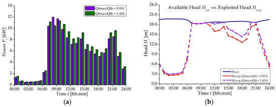
Figure 2.
(a) Produced power Pt; (b) Comparison between available head Ht,av and exploit one Ht,exp—Scenario 1.
Scenario 2: High Available Head Ht,av
- Power Maximization at Qtmax: Qtmax/Qtb = 0.951
In Scenario 2, a higher available head Ht,av was considered. As introduced in Par. 3.1, Qtb = 87.6 L/s and Htb = 95.4 m were calculated by Equations (3) and (7), respectively. From Equation (8), the rotational speed at Qt,max N = 50.5 rps; thus, being N > Nmax, N = Nmax = 50 rps was set. To maximize the produced power, the flow rate ratio Qt,max/Qtb = 0.951 was set obtaining Htb = 94.1 m from Equation (8) and D = 0.240 m from Equation (9), respectively. From Equation (2) φb = 0.128 was thus assessed and the power at BEP Ptb = 64.72 kW was calculated by Equation (5), corresponding to the efficiency at BEP ηtb = 0.80. The maximum produced power at Qt,max of 57.15 kW was thus derived with Equation (4). The rotational speed N able to maximize the power at any time-step was thus derived by Equation (12), resulting N > Nmax from 07:00 to 23:00. For the latter, N = Nmax was thus set. The power number πb and the head number ψb at BEP were estimated equal to 0.66 and 6.44 with Equations (11) and (13), respectively and the flow rate at BEP Qtb, the power at BEP Ptb and the head drop at BEP Htb were obtained from Equations (2), (11) and (13), respectively, at any hourly time-step, as a function of the flowing rate Qt and the corresponding N, being φb, πb and ψb constant at varying N. From Equation (4) the produced power Pt was assessed at any hourly time-step, resulting in the range 2.22 ÷ 57.15 kW. The PAT efficiency ηt, estimated with Equation (5), ranged between 68% and 80%. The daily producible energy of 622.89 kWh/day was thus evaluated. A residual head (Ht,av–Ht,exp) was observed at each time-step. A PRV was combined with PAT to exploit the residual head. Alternatively, multi-stage PATs could be applied for both increasing the hydropower generation and exploiting the residual head.
- Daily Energy Maximization: Qtmax/Qtb = 1.450
By applying the abovementioned procedure setting Qtmax/Qtb = 1.450, results summarized in Table 2 were achieved, compared with those from the Qtmax/Qtb = 0.951 setting. The designed rotational speed N at Qtmax was 36.43 rps with Qtb = 57.5 L/s, Htb = 46.6 m and D = 0.231 m. The produced power at Qtmax was lowered to 50.58 kW, however achieving higher powers at time steps 07:00 and 09:00 (Figure 3). The daily produced energy was higher than that at Qtmax/Qtb = 0.951, being equal to 674.17 kWh/day.
Table 2.
PAT design parameters as a function of Qt,max/Qtb ratio—Scenario 2.
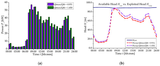
Figure 3.
(a) Produced power Pt; (b) Comparison between available head Ht,av and exploited one Ht,exp—Scenario 2.
Finally, in Figure 4 comparison between the available head Ht,av and the exploited head Ht,exp is plotted at varying the flow rate Qt for both Scenarios and Qtmax/Qtb ratios. In both Scenarios, Qtmax/Qtb = 1.450 resulted in higher Ht,exp, showing a better capability to reduce the exceeding pressure in the WDN. In Scenario 1, the designed PAT was able to exploit the whole exceeding head for flow rates higher than 67 L/s, whereas in Scenario 2, the exceeding head was exploited only at flow rates very close to Qt,max.
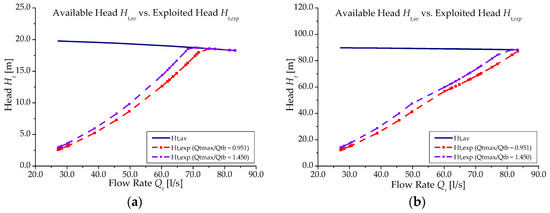
Figure 4.
Comparison between available head Ht,av and exploited one Ht,exp for: (a) Scenario 1; (b) Scenario 2.
4. Conclusions
A procedure for the optimal selection of PATs in WDNs was presented and applied to a WDN to assess its effectiveness at varying the available head in the network. The model was devoted to the preliminary design of PAT main parameters under the hypothesis of Electrical Regulation. Results pointed out that the analytic model is able to assess the operating conditions at BEP, the impeller diameter and the rotational speed, in order to both maximize the power (or the overall producible energy) and regulate the pressure in the network. The procedure can be applied to both single-stage and multi-stage centrifugal PATs, depending on the available head in the network.
Author Contributions
M.G., N.F., F.P. and F.D.P. conceived the treated topic; F.P. and N.F. implemented the model; F.D.P. and G.M. wrote the paper.
Acknowledgments
This work was partly supported by the EU PON/FESR “Ricerca e Competitività” 2007–2013 under projects PON01_01596 “WaterGRID” and PON04a2_F “BE&SAVE e AQUASYSTEM e SIGLOD”.
Conflicts of Interest
The authors declare no conflict of interest.
References
- Binama, M.; Su, W.-T.; Li, X.-B.; Li, F.-C.; Wei, X.-Z.; An, S. Investigation of Pump As Turbine (PAT) technical aspects for micro hydropower schemes: A state-of-the-art review. Renew. Sustain. Energy Rev. 2017, 79, 148–179. [Google Scholar] [CrossRef]
- Pugliese, F.; De Paola, F.; Fontana, N.; Giugni, M.; Marini, G. Experimental characterization of two Pumps As Turbines for hydropower generation. Renew. Energy 2016, 99, 180–187. [Google Scholar] [CrossRef]
- Stepanoff, A.J. Centrifugal and Axial Flow Pumps: Theory, Design and Application; John Wiley & Sons Ed.: New York, NY, USA, 1948. [Google Scholar]
- Fecarotta, O.; Carravetta, A.; Ramos, H.M.; Martino, R. An improved affinity model to enhance variable operating strategy for pumps used as turbines. J. Hydraul. Res. 2016, 54, 332–341. [Google Scholar] [CrossRef]
- Derakhshan, S.; Nourbakhsh, A. Experimental study of characteristic curves of centrifugal pumps working as turbines in different specific speeds. Exp. Therm. Fluid Sci. 2008, 32, 800–807. [Google Scholar] [CrossRef]
- Pugliese, F.; De Paola, F.; Fontana, N.; Giugni, M.; Marini, G. Performance of vertical axis Pumps As Turbines. J. Hydraul. Res. 2018, in press. [Google Scholar] [CrossRef]
- Stefanizzi, M.; Torresi, M.; Fortunato, B.; Camporeale, S.M. Experimental investigation and performance prediction modelling of a single stage centrifugal pump operating as a turbine. Procedia Eng. 2017, 126, 589–596. [Google Scholar] [CrossRef]
- Barbarelli, S.; Amelio, M.; Florio, G. Experimental activity at test rig validating correlations to select pumps running as turbines in microhydro plants. Energy Convers. Manag. 2017, 149, 781–797. [Google Scholar] [CrossRef]
- Fontana, N.; Giugni, M.; Portolano, D. Losses reduction and energy production in Water Distribution Networks. J. Water Res. PL ASCE 2012, 138, 237–244. [Google Scholar] [CrossRef]
- Giugni, M.; Fontana, N.; Ranucci, A. Optimal location of PRVs and turbines in Water Distribution Systems. J. Water Res. PL ASCE 2014, 140, 1–6. [Google Scholar] [CrossRef]
- Jowitt, P.W.; Xu, C. Optimal valve control in water distribution networks. J. Water Res. PL ASCE 1990, 116, 455–472. [Google Scholar] [CrossRef]
- Patelis, M.; Kanakoudis, V.; Gonelas, K. Combining pressure management and energy recovery benefits in water distribution system installing PATs. J. Water Supply Res. Technol. 2017, 66, 520–527. [Google Scholar] [CrossRef]
- Venturini, M.; Alvisi, S.; Simani, S.; Manservigi, L. Energy production by means of Pumps As Turbines in Water Distribution Networks. Energies 2017, 10, 1666. [Google Scholar] [CrossRef]
- Fecarotta, O.; McNabola, A. Optimal location of Pump as Turbines (PATs) in Water Distribution Networks to recover energy and reduce leakage. Water Resour. Manag. 2017, 31, 5043–5059. [Google Scholar] [CrossRef]
- Carravetta, A.; Del Giudice, G.; Fecarotta, O.; Ramos, H.M. Energy production in Water Distribution Networks: A PAT design strategy. Water Resour. Manag. 2012, 26, 3947–3959. [Google Scholar] [CrossRef]
- Carravetta, A.; Del Giudice, G.; Fecarotta, O.; Ramos, H.M. PAT design strategy for Energy Recovery in Water Distribution Networks by Electrical Regulation. Energies 2013, 6, 411–424. [Google Scholar] [CrossRef]
- Balje, O.E. Turbomachines: A Guide to Design, Select and Theory; Wiley-Interscience Ed.: New York, NY, USA, 1981. [Google Scholar]
- Fontana, N.; Giugni, M.; Glielmo, L.; Marini, G.; Zollo, R. Hydraulic and electric regulation of a prototype for real time control of pressure and hydropower generation in a water distribution network. J. Water Res. PL ASCE 2018, in press. [Google Scholar] [CrossRef]
- Yang, S.S.; Derakhshan, S.; Kong, F.Y. Theoretical, numerical and experimental prediction of pump as turbine performance. Renew. Energy 2012, 48, 52–61. [Google Scholar] [CrossRef]
Publisher’s Note: MDPI stays neutral with regard to jurisdictional claims in published maps and institutional affiliations. |
© 2018 by the authors. Licensee MDPI, Basel, Switzerland. This article is an open access article distributed under the terms and conditions of the Creative Commons Attribution (CC BY) license (https://creativecommons.org/licenses/by/4.0/).