Investigation of the Relationship between Three- and One-Dimensional Infiltration Using a Mini Disc Infiltrometer ^†

Abstract

Disc infiltrometer experiments were conducted in the laboratory on two disturbed soils, a loam and a silty clay loam soil, in order to investigate the relationship between three- and one-dimensional infiltration using the proposed equation of Smettem et al. A mini disc infiltrometer of a radius of 45 mm with suction ranged from −5 mm to −70 mm was used. Three- and one-dimensional infiltration tests were performed on repacked cores by applying pressure heads −70, −40 and −10 mm for loam soil, and −30 and −10 mm for silty clay loam soil. Analysis of the results showed that the difference between the three- and one-dimensional infiltration is linear with time confirming the equation of Smettem et al. [1]. Also, this difference is used to calculate the value of an additional infiltration parameter.

1. Introduction

Knowledge of both soil water infiltration characteristics, saturated hydraulic conductivity and soil sorptivity, of the upper soil layers is essential for the modeling of field infiltration process for hydrological applications and agricultural water management.

Tension disc infiltrometers, among other experimental apparatus used in situ for determining these two infiltration characteristics, has been extensively used in last decades [1,2,3,4,5]. Tension disc infiltrometers allow measurements of infiltration with a constant and small negative pressure head, h₀, at the soil surface and has been extensively used to measure the near-saturated hydraulic conductivity, K₀, and sorptivity S₀ [1,2,3,4,5]. Disc infiltrometers have the advantage that are portable and use small volumes of water making them suitable for spatial variability studies [6,7,8].

Various methodologies have been proposed to determine K₀ and S₀ from three-dimensional infiltration data from circular source at soil surface using tension disc infiltrometer. Among these, some are based on steady-state flow data and others on transient flow data [2,4,9,10,11,12,13,14].

In case of steady-state flow from circular source with constant negative pressure head at soil surface, the analytical solution of Wooding [15], is used. Wooding’s equation is applied by assuming that the soil is homogenous and isotropic and the initial water content is uniform. Hydraulic conductivity near saturation can be determined by steady-state infiltration experiments either using multiple-discs with the same pressure head imposed at the surface, or by single-disc infiltration experiments with multiple pressure heads [16]. Wooding’s approach uses a two-parametric model for determining the hydraulic conductivity [17]. However, it is quite difficult to obtain reliable values of sorptivity using infiltration data by disc infiltrometer since there is a difficult to determine the required short time where gravity ignored [12].

Due to uncertainties about the time at which a steady-state infiltration regime is attained, together with the fact that useful information is lost by ignoring the transient stage, several researchers use a transient three-dimensional infiltration equation for disc infiltrometers [18]. Although, several expressions for transient infiltration [3,4,12], have in common the following two-term cumulative infiltration equation analogous to Philip [19],

$$I_{3D}=C_1\sqrt{t}+C_{2}t,$$

(1)

where I is the cumulative infiltration (L) and the subscript 3D refers to three-dimensional infiltration process. The coefficients C₁ (L T-0.5) and C₂ (L T-1) differ among the expressions used [18].

Haverkamp et al. [4], related C₁ and C₂ to S₀ and Κ₀ for short and medium times as follows:

C₁ = S₀,

(2)

$$C_2=\frac{2-\beta }{3}{K}_0+\frac{\gamma S_0^2}{r\left({\theta }_0-{\theta }_n\right)},$$

(3)

where the subscript 0 refers to values on the supply boundary where the pressure head is h₀ (L), n refers to the initial conditions, r is the disc radius (L), β is a shape factor lying between 0 and 1, and γ is a proportionality coefficient. The coefficient γ was originally set equal to $\sqrt{0.3}$ by [1], and later was revised to be 0.6 < γ < 0.8 by [4]. Consequently, the Equation (1) takes the following form:

$$I_{3D}=S_0\sqrt{t}+\frac{2-\beta }{3}{K}_{0}t+\frac{\gamma S_0^2}{r\left({\theta }_0-{\theta }_n\right)}t,$$

(4)

The first term of the right-hand side in Equation (4) represents vertical capillary flow and dominates the infiltration during the initial stage. The second term represents gravity-driven vertical flow and the third term represents lateral capillary flow.

Smettem et al. [1], showed that the additional term accounting for the side effects due the axisymetric flow geometry is linear in time:

$$I_{3D}-I_{1D}=\frac{\gamma S_0^2}{r\left({\theta }_0-{\theta }_n\right)}t,$$

(5)

where the subscript 1D refers to one-dimensional infiltration process.

In order to apply Equation (5) an estimation of C₁ = S₀ and γ is required.

However, Vandervaere et al. [5], had reported that the calculation of C₁ and C₂ parameters by direct nonlinear fitting of Equation (1) on experimental data can provide fitted values for C₁ and C₂, even if these values have no physical meaning, e.g., negative C₂ value. So, negative K₀ is a physical impossibility indicating a problem with the data set. To overcome this problem, various linear fitting techniques of Equation (1) have been proposed to detect possible inadequacy of Equation (1), as well as scattering of data points.

Smiles and Knight [20], proposed linearizing of Equation (1) by dividing both sides by $\sqrt{t}$, giving the equation:

$$\frac{I_{3D}}{\sqrt{t}}=C_1+C_2\sqrt{t},$$

(6)

and then plotting $I_{3D}/\sqrt{t}$ as a function of $\sqrt{t}$. Thus, it is easy to determine C₁ = S₀ as the intercept and C₂ as the slope of the fitted line on experimental data. Also, S₀ could be estimated from cumulative one-dimensional infiltration data versus square root of time, at short times, where this relationship is linear with slope S₀.

The main purpose of this study is to investigate the difference between three- and one-dimensional infiltration on two disturbed soils, a loam and a silty clay loam soil, using a mini disc infiltrometer and to compare this difference with the proposed equation of Smettem et al. [1].

2. Materials and Methods

A mini disc infiltrometer [21], with a radius of 22.5 mm was used to perform three-dimensional infiltration experiments on repacked soils into a cylinder of 300 mm diameter and 300 mm length and the disc was placed in the center of the box to allow fully unconfined three-dimensional flow. On the other hand, one-dimensional infiltration experiments were performed on repacked soils into a cylinder of 45 mm diameter and 500 mm length and the disc was placed on the top surface of the soils.

The soils examined were a Loam (L) and a Silty Clay Loam (SiCL). The soil texture and the bulk density, ρ_φ, of soils are presented in

Table 1. Soil particle size distribution and bulk density, ρ_φ, of the soils examined.

Soil Type	Clay (%)	Silt (%)	Sand (%)	ρφ (g.cm−3)
L	20.0	38	42.0	1.17
SiCL	36.5	52	11.5	1.23

. The disturbed soil samples used had been air dried before the beginning of the experiments and consequently the initial soil water content was very low (θ_n = 0.04 cm³ cm⁻³ for both soils). The pressure heads applied, during the three- and one-dimensional infiltration tests, were −70, −40 and −10 mm for the L soil, and −30 and −10 mm for the SiCL soil. After cessation of each infiltration experiment, soil samples were obtained to determination soil water content.

The duration of the experiments ranged from 600 to 900 s. The sorptivity S₀ value for each pressure head h₀ was obtained by plotting one-dimensional infiltration data $I_{1D}$ as a function of $\sqrt{t}$, for short times up to 60 s where the $I_{1D}\left(\sqrt{t}\right)$ relationship is linear.

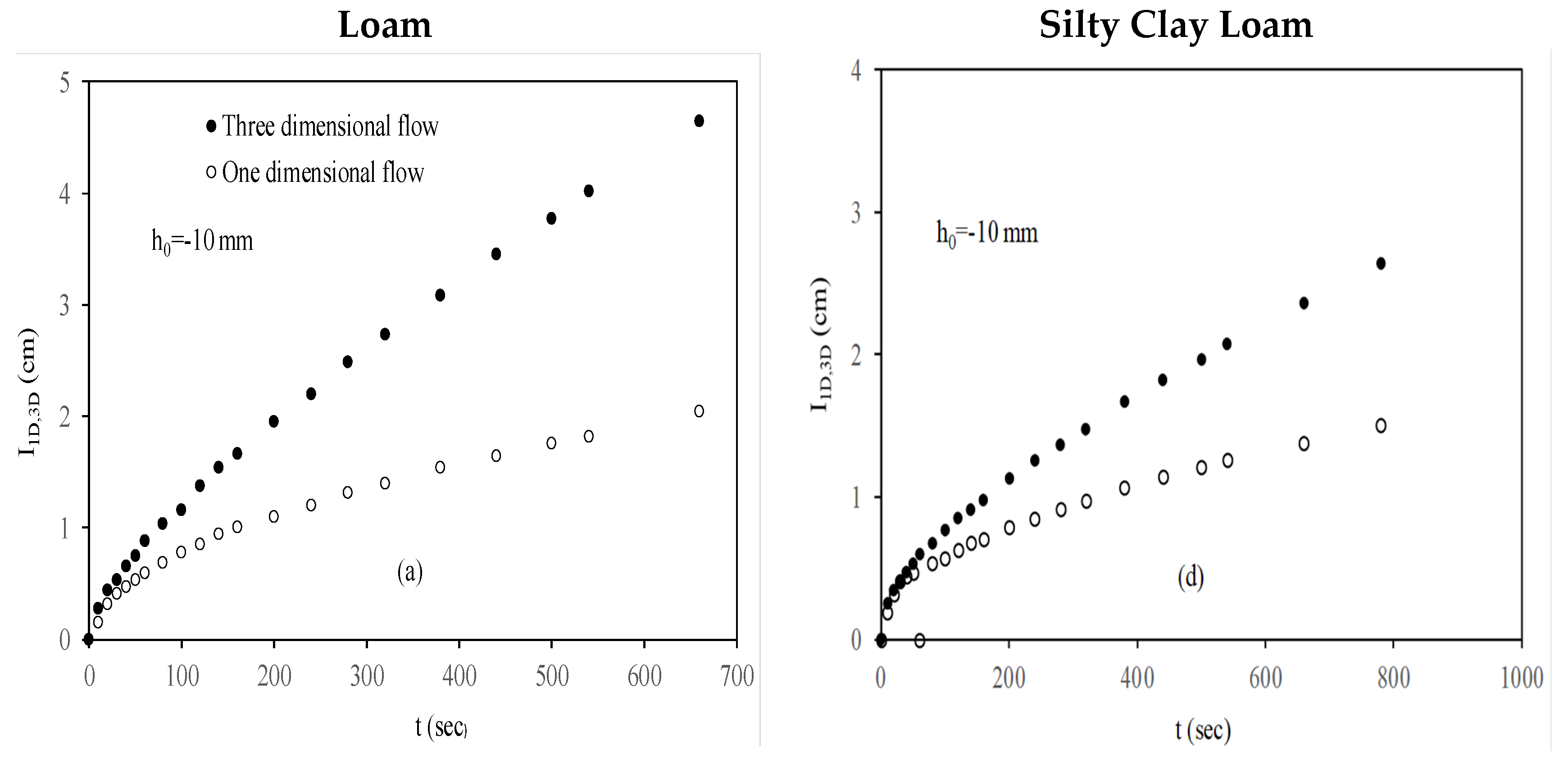
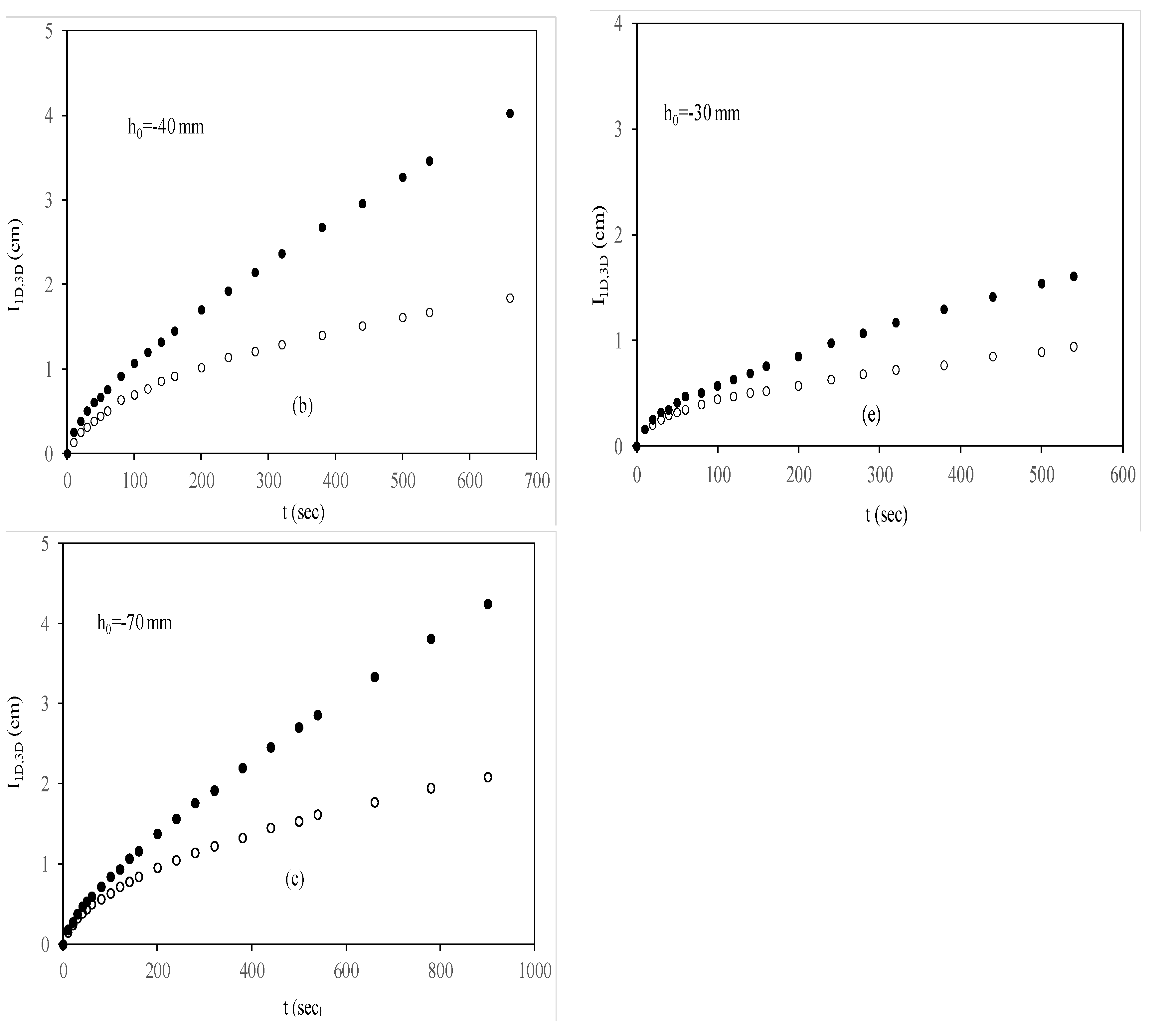
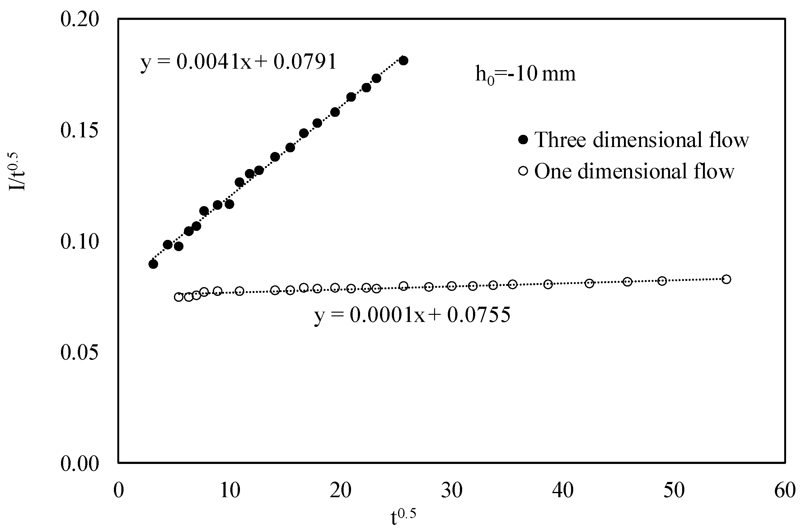
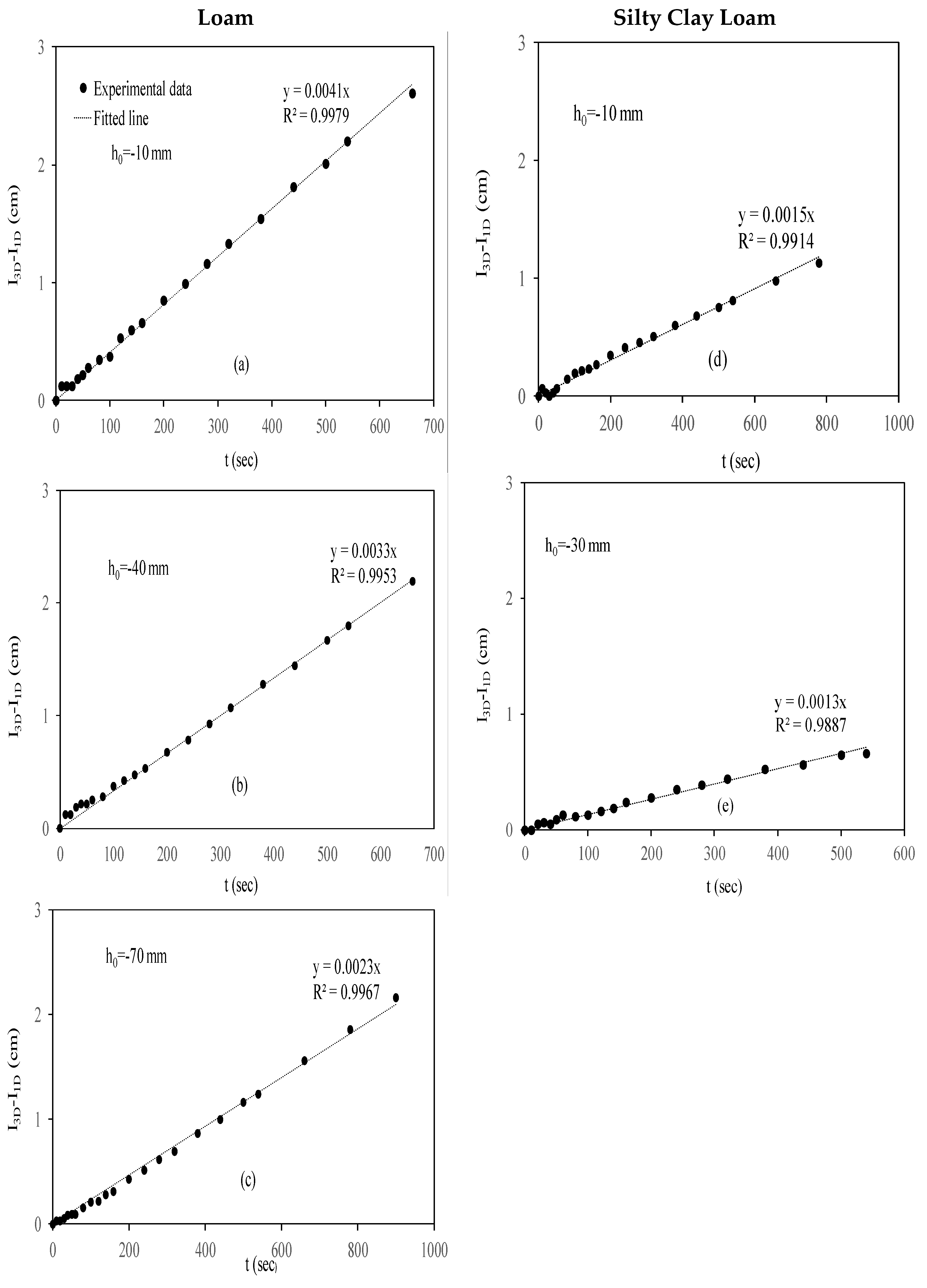
3. Results and Discussion

In Figure 1, three- and one-dimensional infiltration relationships are depicted for L and SiCL soils for each pressure head used.

At short times ($t\to 0$), the sorptivity S₀ can be calculated by the equation $I_{3D}=I_{1D}=S_0\sqrt{t}$. However, Smettem [22], and Minasny and McBratney [23], showed that the classical approach to calculate sorptivity from a disk infiltrometer experiment (three-dimensional infiltration flow) may give erroneous result (overestimated). For this reason, S₀ value, for each pressure head, was obtained from the slope of the linear relationship of the one-dimensional infiltration data versus square root of time, $I_{1D}\left(\sqrt{t}\right)$, (data not shown) for short times where the effect of the gravity is negligible (

Table 2. Parameters of one-dimensional infiltration experiment for loam (L) and silty clay loam (SiCL) soil and the coefficient of determination R² between the experimental infiltration data $I_{1D}\left(\sqrt{t}\right)$ and fitted curve for S₀ estimation.

Soil Type	Pressure Head, h0 (mm)	Water Content, θ0 (cm3cm−3)	Soil Sorptivity, S0 (cm s−0.5)	R2
L	−10	0.385	0.072	0.970
	−40	0.369	0.063	0.958
	−70	0.362	0.058	0.986
SiCL	−10	0.464	0.061	0.990
	−30	0.446	0.046	0.990

).

The one-dimensional infiltration data were used in contrast to the three-dimensional infiltration data, since the corresponding time where the $I_{3D}\left(\sqrt{t}\right)$ function is linear, is much shorter and therefore is uncertain in estimation of S₀ [4]. The choice of the appropriate time interval for calculating S₀ in the one-dimensional infiltration experiments, where the soils used are fine-textured and disturbed, is relatively easy since no sand layer is needed to be used on the surface of each porous medium to ensure hydraulic contact between the infiltrometer and the soil. The presence of this layer can be affect on the first stages of infiltration making difficult the estimation of the appropriate time interval for calculating S₀ [5,24]. The value of S₀ at each pressure head can also be calculated by linearization methodologies of the Equation (1) using one- or three-dimensional infiltration data [5,20,22]. The applied methodology, in this study, for estimation of S₀ value for each pressure head compared with the aforementioned linearization method gave similar results. Perroux and White [25], after conducting disc infiltrometer experiments, showed that the time for estimating S₀ depends on the soil type and ranged from 6 to 2450 s with an average value of 60 s.

In Figure 2, the fitted curves of the linear relationship $\frac{I}{\sqrt{t}}=C_1+C_2\sqrt{t}$ on the three- and one-dimensional infiltration data using pressure head h₀ = −10 mm, for the Loam soil, are presented. Similar results obtained using the other pressure heads for both soils (data not shown).

As shown in Figure 2, both fitting functions (i.e., on three- and one-dimensional infiltration data) have almost the same intercept value C₁ = S₀ [13]. The intercept values for all pressure heads tested in the two soils were very close to S₀ values obtained from the slope of the linear relationship of the one-dimentional infiltration data versus square root of time, $I_{1D}\left(\sqrt{t}\right)$, and are presented in Table 2. Vandervaere et al. [13], report that a difference up to 15% between S₀ values obtained from three- and one-dimensional infiltration is acceptable due to possible different soil packing.

In Figure 3, the difference between three- and one-dimensional infiltration (I_3D–I_1D) as a function of time t, for each pressure head tested in the two soils, is presented. As shown the difference I_3D-I_1D is linear in time t for all cases studied, with a coefficient of determination R² > 0.99, as predicted by the Equation (5) of Smettem et al. [1], and independent of gravity. It also appears that the slope of this linear function decreases by reducing the pressure head. This practically means that the reduction of S₀ is greater than the difference of soil water content θ₀–θ_n.

The comparison between the experimental relationship I_3D–I_1D(t) and the predicted one by the Equation (5) showed a very good agreement for the proportionality constant γ = $\sqrt{0.3}$, for both porous media used. This value of γ parameter is given in the model of Smettem et al. [1]. However, the value of γ = 0.75 was suggested by [1], as a result of the comparison between experimental and analytical results in the case of a sandy loam soil. This difference of γ values was attributed to the use of sharp wetting front approximation in developing the analytical solution. Haverkamp et al. [4], reported that in normal working conditions are reasonably bounded by 0.6–0.8. In addition, Smettem et al. [22], using a double disc tension infiltrometer in three- and one-dimensional infiltration experiments on a sandy loam soil with pressure head h₀ = −30 mm, found a value of γ = 0.726.

The difference between the experimental value of γ of our study and those ones are referred in the works of [4], and [22], can be attributed to various factors such as soil type, initial and boundary conditions, as well as radius of infiltrometer.

4. Conclusions

The difference between three- and one-dimensional infiltration flow (I_3D–I_1D) is proportional to time as predicted by the equation of Smettem et al. [1]. However, the coefficient γ is different from that calculated from other experiments on different soils using different infiltrometers. The calculation of γ value, in combination with the value of S₀, as calculated by various methodologies, can be used to calculate the contribution of gravitational flow during three-dimensional infiltration.

References

1. Smettem, K.R.J.; Parlange, J.-Y.; Ross, P. J.; Haverkamp, R. Three-dimensional analysis of infiltration from the disc infiltrometer: 1. A capillary-based theory. Water Resour. Res. 1994, 30, 2925–2929. [Google Scholar] [CrossRef]
2. Smettem, K.R.J.; Clothier, B.E. Measuring unsaturated sorptivity and hydraulic conductivity using multiple disc permeameters. J. Soil Sci. 1989, 40, 563–568. [Google Scholar] [CrossRef]
3. Warrick, A.W. Models for disc infiltrometers. Water Resour. Res. 1992, 28, 1319–1327. [Google Scholar] [CrossRef]
4. Haverkamp, R.; Ross, P.J.; Smettem, K.R.J.; Parlange, J.-Y. Three dimensional analysis of infiltration from disc infiltrometer 2. Physically-based infiltration equation. Water Resour. Res. 1994, 30, 2931–2935. [Google Scholar] [CrossRef]
5. Vandervaere, J.P.; Vauclin, M.; Elrick, D.E. Transient flow from tension infiltrometers: I. The two parameter equation. Soil Sci. Soc. Am. J. 2000, 64, 1263–1272. [Google Scholar] [CrossRef]
6. Smettem, K.R.J. Characterization of water entry into a soil with a contrasting textural class: Spatial variability of infiltration parameters and influence of macroporosity. Soil Sci. 1987, 144, 167–174. [Google Scholar] [CrossRef]
7. Mohanty, B.P.; Ankeny, M.D.; Horton, R.; Kanwar, R.S. Spatial analysis of hydraulic conductivity measured using disc infiltrometers. Water Resour. Res. 1994, 30, 2489–2498. [Google Scholar] [CrossRef]
8. Shouse, P.J.; Mohanty, B.P. Scaling of near-saturated hydraulic conductivity measured using disc infiltrometers. Water Resour. Res. 1998, 34, 1195–1205. [Google Scholar] [CrossRef]
9. Clothier, B.E.; White, I. Measurement of sorptivity and soil water diffusivity in the field. Soil Sci. Soc. Am. J. 1981, 45, 241–245. [Google Scholar] [CrossRef]
10. Ankeny, M.D.; Ahmed, Μ.; Kaspar, T.C.; Horton, R. Simple field method for determining unsaturated hydraulic conductivity. Soil Sci. Soc. Am. J. 1991, 55, 467–470. [Google Scholar] [CrossRef]
11. Reynolds, W.D.; Elrick, E.D. Determination of hydraulic conductivity using a tension infiltrometer. Soil Sci. Soc. Am. J. 1991, 55, 633–639. [Google Scholar] [CrossRef]
12. Zhang, R. Infiltration models for the disc infiltrometer. Soil Sci. Soc. Am. J. 1997, 61, 1597–1603. [Google Scholar] [CrossRef]
13. Vandervaere, J.P.; Vauclin, M.; Elrick, D.E. Transient flow from tension infiltrometers: II. Four Methods to Determine Sorptivity and Conductivity. Soil Sci. Soc. Am. J. 2000, 64, 1272–1284. [Google Scholar] [CrossRef]
14. Latorre, B.; Moret-Fernández, D.; Peña, C. Estimate of soil hydraulic properties from disc infiltrometer three-dimensional infiltration curve: Theoretical analysis and field applicability. Proced. Environ. Sci. 2013, 19, 580–589. [Google Scholar] [CrossRef]
15. Wooding, R.A. Steady infiltration from shallow circular pond. Water Resour. Res. 1968, 4, 1259–1273. [Google Scholar] [CrossRef]
16. Lazarovitch, N.; Ben Gal, A.; Simunek, J.; Shani, U. Uniqueness of soil parameters determined by a combined Wooding inverse approach. Soil Sci. Soc. Am. J. 2007, 71, 860–865. [Google Scholar] [CrossRef]
17. Gardner, W.R. Some steady-state solutions of the unsaturated moisture flow equation with application to evaporation from a water table. Soil Sci. 1958, 85, 228–232. [Google Scholar] [CrossRef]
18. Vandervaere, J.P. The soil solution phase. In Methods of Soil Analysis: Part 4, Physical Methods; Dane, J.H., Topp, G.C., Eds.; SSSA, Inc.: Madison, WI, USA, 2002; pp. 889–894. [Google Scholar]
19. Philip, J.R. The theory of infiltration: 4. Sorptivity and algebraic infiltration equations. Soil Sci. 1957, 84, 257–264. [Google Scholar] [CrossRef]
20. Smiles, D.E.; Knight, J.H. A note on the use of the Philip infiltration equation. Aust. J. Soil Res. 1976, 14, 103–108. [Google Scholar] [CrossRef]
21. Mini Disc Infiltrometer, User’s Manual; Decagon Devices Inc.: Pullman, DC, USA, 2007; 24p.
22. Smettem, K.R.J.; Ross, P. J.; Haverkamp, R.; Parlange, J.-Y. Three-dimensional analysis of infiltration from the disc infiltrometer: 3. Parameter estimation using a double-disk tension infiltrometer. Water Resour. Res. 1995, 10, 2491–2495. [Google Scholar] [CrossRef]
23. Minasny, B.; McBratney, A.B. Estimation of sorptivity from disc-permeameter measurements. Geoderma 2000, 95, 305–324. [Google Scholar] [CrossRef]
24. Vandervaere, J.P.; Peugeot, C.; Vauclin, M.; Angulo-Jaramillo, R.; Lebel, T. Estimating hydraulic conductivity of crusted soils using disc infiltrometers and minitensiometers. J. Hydrol. 1997, 188–189, 203–223. [Google Scholar] [CrossRef]
25. Perroux, K.M.; White, I. Designs for disc permeameters. Soil Sci. Soc. Am. J. 1988, 52, 1205–1215. [Google Scholar] [CrossRef]
Figure 1. Representation of three- and one-dimensional experimental infiltration data with time, I1D,3D(t), for various pressure heads: (a) h0 = −10 mm; (b) h0 = −40 mm; (c) h0 = −70 mm for Loam soil, and (d) h0 = −10 mm; (e) h0 = −30 mm for Silty Clay Loam soil.
Proceedings 02 00660 g001aProceedings 02 00660 g001b
Figure 2. Linear representation of three- and one-dimensional experimental infiltration data and fitted linear lines for pressure head h0 = −10mm, for Loam soil.
Proceedings 02 00660 g002
Figure 3. The difference between three- and one-dimensional infiltration flow over time, for pressure heads: (a) h0 = −10 mm; (b) h0 = −40 mm; (c) h0 = −70 mm for Loam soil, and (d) h0 = −10 mm; (e) h0 = −30 mm for Silty Clay Loam soil. The fitted line is from Equation (5).
Proceedings 02 00660 g003