Bivariate Flood Frequency Analysis Using Copulas ^†

Abstract

Flood frequency estimation for the design of hydraulic structures is usually performed as a univariate analysis of flood event magnitudes. However, recent studies show that for accurate return period estimation of the flood events, the dependence and the correlation pattern among flood attribute characteristics, such as peak discharge, volume and duration should be taken into account in a multivariate framework. The primary goal of this study is to compare univariate and joint bivariate return periods of floods that all rely on different probability concepts in Yermasoyia watershed, Cyprus. Pairs of peak discharge with corresponding flood volumes are estimated and compared using annual maximum series (AMS) and peaks over threshold (POT) approaches. The Lyne-Hollick recursive digital filter is applied to separate baseflow from quick flow and to subsequently estimate flood volumes from the quick flow timeseries. Marginal distributions of flood peaks and volumes are examined and used for the estimation of typical design periods. The dependence between peak discharges and volumes is then assessed by an exploratory data analysis using K-plots and Chi-plots, and the consistency of their relationship is quantified by Kendall’s correlation coefficient. Copulas from Archimedean, Elliptical and Extreme Value families are fitted using a pseudo-likelihood estimation method, verified using both graphical approaches and a goodness-of-fit test based on the Cramér-von Mises statistic and evaluated according to the corrected Akaike Information Criterion. The selected copula functions and the corresponding joint return periods are calculated and the results are compared with the marginal univariate estimations of each variable. Results indicate the importance of the bivariate analysis in the estimation of design return period of the hydraulic structures.

1. Introduction

Hydrological frequency analysis is an important area of hydraulic engineering design, water resources planning and management. This involves the selection of the variables of interest, the sampling of a sample series and the choice of the most appropriate population distribution. Traditionally, rainfall and flood frequency analysis has been performed using the assumption that the different variables (i.e., intensity, depth, duration and discharge, volume, duration) are independent. However, in most cases this assumption is not valid. For instance, different pairs of flood peaks and flood volumes may cause an equal raise in the river’s water levels and therefore the performance of univariate analysis may not be sufficient. This interdependency of hydrological variables urged scientists and water managers to derive a joint law in order to successfully describe the main characteristics of the observed hydrological events. The first bivariate frequency distributions were generated based to the hypothesis that the variables of interest either have the same marginal probability distribution, or that their joint relationship is normally distributed (or become normally distributed after a transformation) [1]. These assumptions, however, were not always valid and therefore led to uncertainties in the estimation of hydrological values. In recent years, several studies were focused in finding a method which would assess in the investigation of the statistical behavior of dependent hydrological variables, without the need of the assumptions that classical bivariate frequency distributions use. The first paper on copulas in hydrology was published by De Michele and Salvadori [2], and in the next few years, several other studies further expanded the theory, such as Favre et al. [3]; Salvadori and De Michele [4], Salvadori and De Michele [5] and Genest and Favre [6].

The main concept of the copula approach is that a joint distribution function can be divided into two independent parts, the one describing the marginal-univariate behavior and the other the dependence structure [7,8]. Copulas are the functions that describe the dependence between random variables and as a result, are able to couple the marginals of these variables into their joint distribution function [9]. The importance of this approach in the field of engineering and water science is noticeable. Copula method offers an efficient way in finding reasonable multivariate estimates for hydrological events that have a certain likelihood of occurrence. These estimates are used as design variables of the hydraulic structures. Design variables are characterized by a return period (recurrence interval) defined as the average time elapsing between two successive realizations of an event whose magnitude exceeds a defined threshold [10,11]. In practice, the selection of a reliable return period is crucial as it is the fundamental parameter in the design of hydraulic structures.

The objective of the present study is to present in short the successive steps needed to build a copula model for hydrological variables and to calculate and compare the obtained univariate and joint bivariate return periods. The results of this work are also expected to investigate the deviations among the estimated design values when choosing different sampling methods. With the marginal distributions selected according to the methodology of traditional univariate analysis using two different types of extreme events peak series, a set of copula based bivariate distributions for peak flow–flood volume are determined. Univariate and joint bivariate return periods are then estimated for the daily datasets of stream flow. A brief overview of the case study and the details of the copula theory and the description of the approach are presented in the Data and Methodology section. This will introduce the Results section, in which the basic outputs of this work will be presented along with a comparison of the estimated univariate and bivariate return periods for each case. Finally, a short discussion of the results will be then made in the Conclusion chapter.

2. Data and Methodology

2.1. Data

Yermasoyia Basin is located in the southern side of mountain Troodos of Cyprus, roughly 5 km north of Limassol city and feeds one of 108 reservoirs of the island. The watershed area is 157 km² and its elevation ranges from 70 m up to 1400 m. The length of the main stream of the basin is about 25 km [12] and the average basin wide annual precipitation is 640 mm, ranging from 450 mm at the low elevations up to 850 mm at the upper parts of the watershed. The 65% of the mean annual runoff is generated by rainfall during winter months. The river is usually dry during summer months and the peak flows are observed in winter months and produced by rainfall events. Thirty years of daily discharge data (October 1970–September 1999) collected from the hydrological station on the Yermasoyia River were used for this study. The observed runoff data corresponds to the outlet of the basin, and measurements are collected prior to the dam construction. The mean annual discharge is 0.38 m³/s and the baseflow to total stream flow is 52% for the period of study.

2.2. Methodology

This study’s primary objective is the application of the copula method and the evaluation of its results. To that end, approaches to specify the marginal distribution functions for the different variables were initially applied. This includes data analysis and implementation of baseflow separation using Lyne-Hollick filtering method [13], modeling extremes for the selected parameters via the annual maxima and the peaks of threshold methods and finally, finding the appropriate distributions for each variable of interest. Afterwards, the return periods for each variable were calculated based to the typical univariate approach.

As previously stated, for the copula approach to be performed the dependence between the two variables of interest needed to be assessed. This could be done either by visualizing dependence or by the performance of statistical tests. The Chi-plot and K-plot are the most common graphical tools for detecting dependence. The statistical tests of dependence were performed by computing Kendall‘s correlation coefficient (Kendall’s tau) and both graphical methods were taken into consideration for better visualization of the results.

After the dependence between the variables was evaluated, copulas from three different families were selected as candidate models. In the present work we considered only bivariate distributions and made use of Archimedean (Gumbel–Hougaard, Clayton, Frank and Joe), extreme value (Gumbel–Hougaard and Tawn) and elliptical (Normal or Gaussian) models. The maximization of the pseudolikelihood, a generally applicable method which does not have limitations regarding the dependence parameter, was selected for estimating the model’s parameters for this study. The exclusion of non-admissible copulas was based to Cramér-von Mises statistic test, computed using a bootstrap procedure as described in Genest et al. (2009) [14]. Graphical tests for a visual description of the copula fitting and complementary analysis were also used. Finally, the (corrected) Akaike Information Criterion (AIC) [15,16] among the non-rejected copulas determined the most appropriate model.

After the choice of the most efficient copula model, the bivariate distributions needed to be constructed. A copula is a joint distribution function of standard uniform random variables able to connect univariate marginal distribution functions with the multivariate probability distribution, as stated in Sklar Theorem [9]:

Let F_XY be a joint distribution function with marginals F_X and F_Y. Then there exists a copula C such that:

F_XY (x, y) = C(F_X (x), F_Y (y)),

(1)

for all reals x, y. If F_X, F_Y are continuous, then C is unique; otherwise, C is uniquely defined on Range (F_X) × Range (F_Y). Conversely, if C is a copula and F_X, F_Y are distribution functions, then F_XY given by Equation (1) is a joint distribution function with marginals F_X and F_Y.

After modeling the bivariate distribution the copula based return periods were computed. In this study the bivariate joint (primary) return periods called OR operator “∨” (union of events - either of the variables u and v exceed the defined thresholds) and AND operator “∧” (intersection of events—both of the variables u and v exceed the defined thresholds) [5,10], were computed and are defined as:

$$T_{u,v}^{OR}=\frac{\mu }{1-C_{u,v}\left(u,v\right)},$$

(2)

$$T_{u,v}^{AND}=\frac{\mu }{1-u-v+C_{u,v}\left(u,v\right)},$$

(3)

where u and v follow a uniform distribution U(0, 1). The U denotes F_X(X) and V denotes F_Y(Y) and were constructed after applying the probability integral transform to X and Y, a transformation which allowed us to simplify our work by using an equivalent set of values which follow the standard uniform distribution.

In comparison to the univariate return periods, the joint bivariate estimates are not unique, but instead, they have infinite combinations of values, described with the level curve. All pairs (u, v) that lie on the same level curve of the copula have the same return period T(p), however, these combinations of values for u and v have various probabilities of occurrence and can have significant differences from one another. For the purposes of the present study the most-likely design realization method [17], was used to select a unique return period. This method introduces a weighting function which specifies the point over the critical layer with the greatest value of the joint probability density function f_xy. It is also known as “typical” critical realization, and is described with the following equation:

$$\left(u,v\right)=\underset{C\left(u,v\right)=t}{\underbrace{argmax}}{f}_{XY}\left( F_x^{-1}\left(u\right),F_Y^{-1}\left(v\right)\right),$$

(4)

where u and v depict the converted via the probability integral transform realizations of the marginal distributions F_X and F_Y of the random variables X and Y. After the identification of the maximization point, the pair (u, v) was used in order for the exceedance probability to be calculated. As a final step, a comparison of the different return periods coming from univariate and bivariate analysis was performed in order to investigate the results of the copula method.

3. Results

In order to evaluate the design variables, which could be used in the sizing of a flood control reservoir on the Yermasoyia River, the technique described in the methodology section was applied. In this case, both the flood peak and the flood volume are crucial factors; thus, provided that the two variables are related, the copula approach would be more substantial than the single-variate one. The flow peaks Q were initially selected based on the annual maximum series method. The Lyne-Hollick baseflow separation filter was applied in order to separate the baseflow from the total flow. The remaining values constitute the runoff or hydrograph volume. Then, the flood volume V was estimated by finding the flood volume which corresponds to the selected flood peaks events. As a second approach, the peaks over threshold (POT) method was also applied in the Yermasoyia flow dataset. The threshold was chosen according to the POT methodology, aiming to create a larger sample of extreme events compared to the previous analysis. More specifically, the threshold u₀ = 3.8 m³/s was selected in order to satisfy the two graphical criteria; above the threshold u₀, i. the mean residual life plot should be approximately linear in u and ii. the values of shape ξ and scale σ in the threshold range plot for parameters should be stabilized. The available observations amount to n = 40 pairs of maximum flow peaks (Q) with a mean inter-arrival time μ = 0.75 years. The sampled peak discharge series are presented in Figure 1a,b. Afterwards, the flood volumes (V) corresponded to the specified flood peaks were calculated.

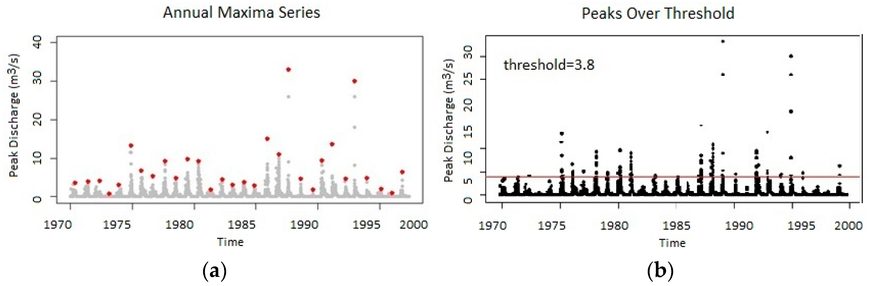
3.1. Univariate Analysis

After the selection of extreme events, a univariate flood and rainfall frequency analysis was performed. Different probability models such as Generalized Extreme Values (GEV), Gumbel (EVI) and Generalized Pareto Distribution (GPD) for peak discharge and GEV, Gamma, Exponential, and Log-normal for flood volumes were applied to the datasets. The distribution’s parameters were estimated with the help of maximum likelihood method, a method which will be as well used in copula‘s parameters estimation process [18]. Subsequently, the Kolmogorov-Smirnov Goodness-of-Fit and graphical tests were produced to select the distributions that produced an adequate fit to the data and finally, AIC [15] values among the non-rejected copulas determined the most appropriate statistical model. For the first set of data, the generalized extreme value distribution (GEV) was selected for fitting. Then, the events which were chosen using a POT approach were fitted in a Generalized Pareto Distribution (GPD) in accordance to extreme value theory. After the graphical and Goodness of Fit (GOF) tests were performed and AIC values were computed for each of the accepted models, exponential and lognormal distributions were selected for the flood volumes V, for the first and second dataset respectively. Model parameters were estimated by maximum likelihood (ML) method. Finally, as soon as the appropriate model was obtained, the univariate return periods were calculated for 2, 5, 10, 25, 50, 100, 200 and 500 years and are presented in

Table 1. Results of the Univariate Return Periods 2, 5, 10, 25, 50, 100, 200 and 500 for Peak Discharge and Flood Volume for Annual Maximum Series (AMS) and Peaks Over Threshold (POT), Yermasoyia Station.

Return Level (Years):	2	5	10	25	50	100	200	500
AMS Sampling
Peak Discharge (m3/s)	5.14	10.34	15.53	25.09	35.28	49.05	67.73	103.01
Flood Volume (106 m3)	1.26	2.93	4.20	5.87	7.13	8.39	9.66	11.33
POT Sampling
Peak Discharge (m3/s)	1.77	5.37	9.53	18.01	27.81	41.97	62.44	104.12
Flood Volume (106 m3)	1.43	2.58	3.52	4.89	6.05	7.32	8.72	10.79

. The estimated univariate return values have differences only for the peak discharge variable in the lower return periods (Table 1). However, the deviations between the two approaches could be attributed to the data processing algorithm, and not solely to the applied methodology.

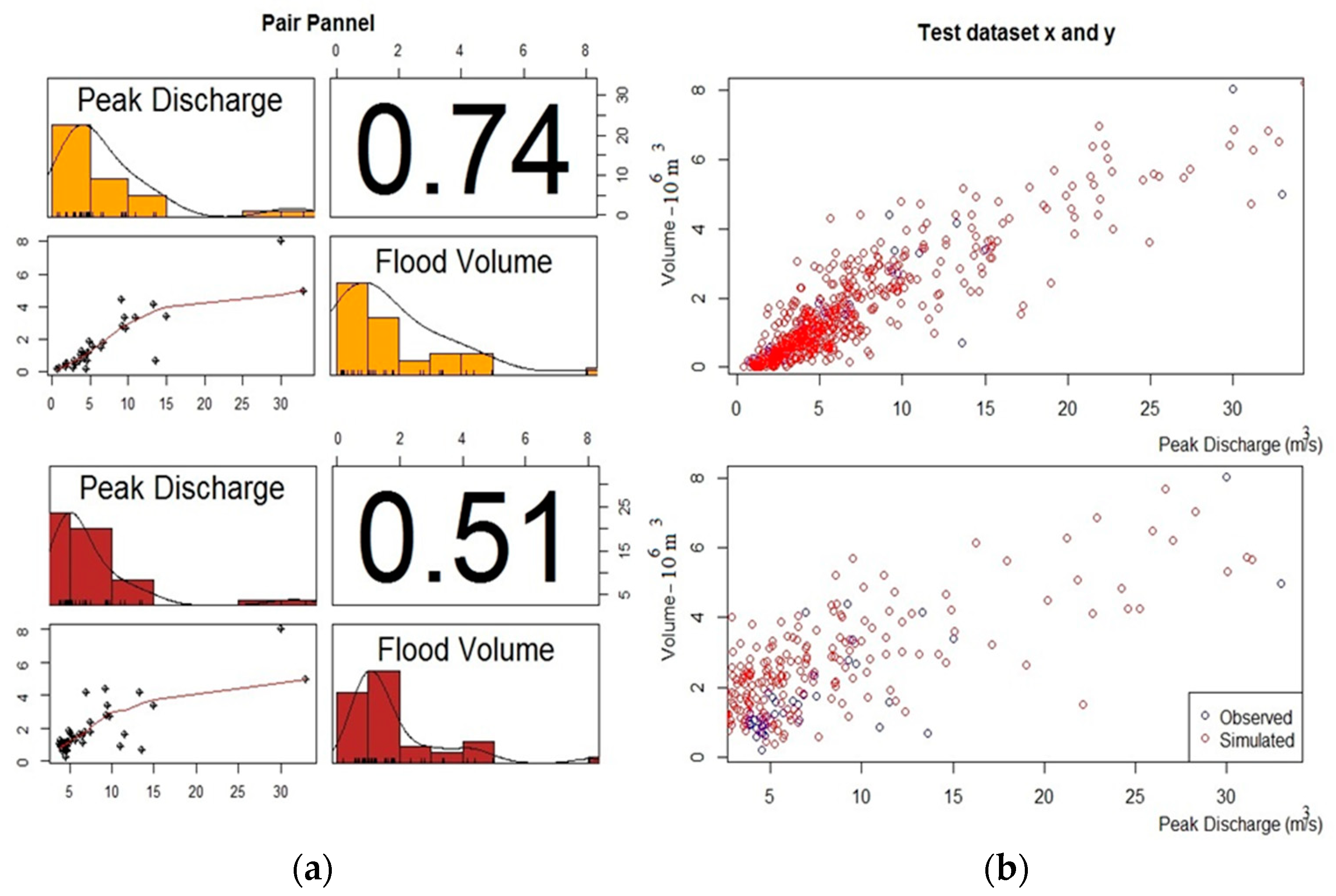
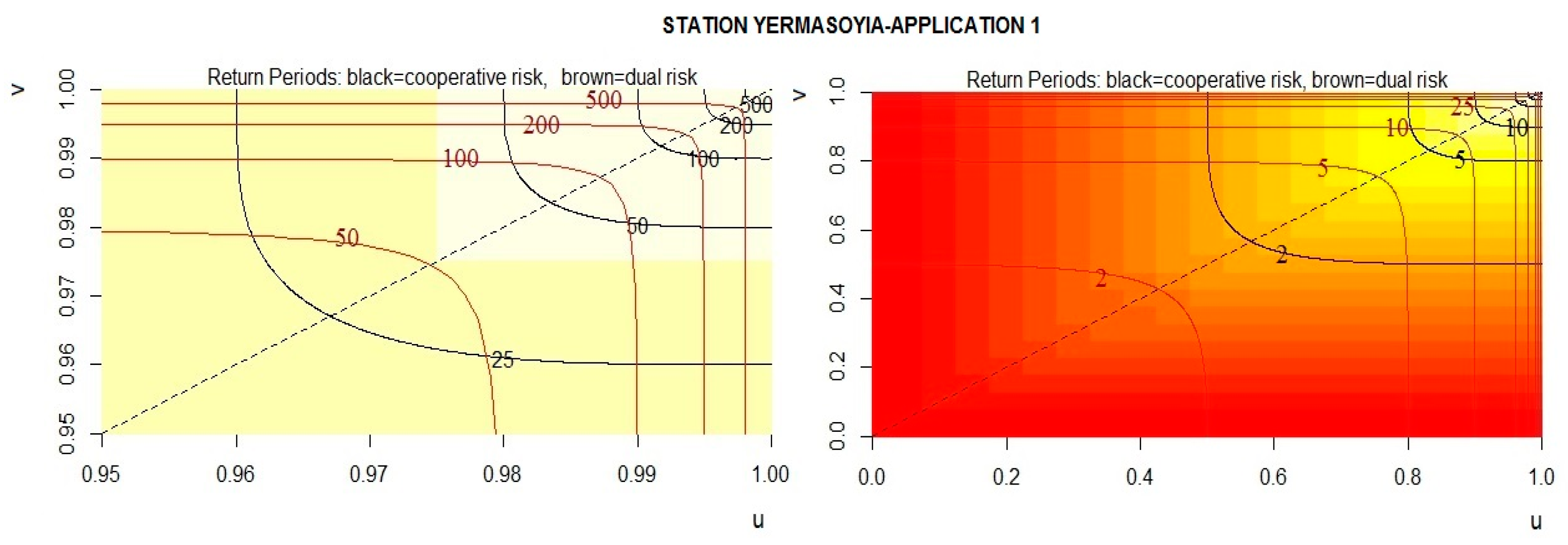
3.2. Bivariate Analysis

After the univariate analysis was performed, a formal assessment of the dependence between the pairs of the considered variables was tested with the help of Kendall correlation coefficient. The values returned were 0.74 for the first sample (AMS sampling for peak discharge) and 0.51 for the second (POT sampling for peak discharge). Histograms and a scatterplot of the Q-V pair are presented in Figure 2a, in which a strong correlation between the two variables can be easily noticed.

In the next step, the different copulas from the three families were fitted to Q-V pair. The parameters of the copulas were estimated with the maximum pseudolikelihood method and the considered functions were compared with different goodness-of-fit tests. For the AMS method sample only Tawn and Survival Gumbel copulas were rejected while for the POT sample, all copula candidate models were accepted in the 95% significance level. Gumbel copula with parameter = 3.51 was selected for the AMS sample, as it had the lowest AIC value, and at the same time had an adequate fit. The statistical test p-value was 0.053 for the bootstrapped p-value of the goodness-of-fit test using the Cramer-von Mises statistic (95% significance level). In a similar manner, the Joe Copula (parameter = 2.78) for the POT method was fitted to the sample (p-value = 0.511). Furthermore, Figure 2b shows the graphical tests of the selected copulas Gumbel and Joe for a sample size of 1000 simulations for the pair (Q-V). The Kendall‘s tau extracted from the comparison between observed and simulated values was 0.71 for the copula and 0.74 for the actual data in the first case, and 0.49 with 0.51 for the second, indicating that the correlation of the real data was preserved in the copula.

After copula selection, the bivariate distribution function was constructed and the selected marginals were taken into consideration. Figure 3 illustrates the level curves for the bivariate return periods (application 1). The results are presented for demonstrational purposes. Finally,

Table 2. Results of the Bivariate Return Periods 2, 5, 10, 25, 50, 100, 200 and 500 for Peak Discharge and Flood Volume using Annual Maximum Series (AMS) method.

Return Level (Years):	2	5	10	25	50	100	200	500
AMS Sampling
Peak Discharge/dual (m3/s)	4.46	8.98	13.53	21.87	31.14	43.41	58.01	93.07
Peak Discharge/cooperative (m3/s)	5.86	11.47	17.07	27.39	38.42	53.35	75.06	108.06
Flood Volume/dual (106 m3)	1.01	2.59	3.82	5.49	6.72	7.98	9.34	10.84
Flood Volume/cooperative (106 m3)	1.53	3.28	4.57	6.26	7.52	8.78	9.99	11.93

and

Table 3. Results of the Bivariate Return Periods 2, 5, 10, 25, 50, 100, 200 and 500 for Peak Discharge and Flood Volume using Peaks over Threshold (POT) method.

Return Level (Years):	2	5	10	25	50	100	200	500
POT Sampling
Peak Discharge/dual (m3/s)	1.77	5.18	8.82	15.25	22.21	31.89	44.69	70.86
Peak Discharge/cooperative (m3/s)	5.31	8.80	12.69	20.92	30.85	45.56	66.26	110.35
Flood Volume/dual (106 m3)	0.28	1.16	2.43	4.22	5.53	6.88	8.36	10.47
Flood Volume/cooperative (106 m3)	1.46	2.68	3.72	5.32	6.67	8.12	9.79	12.00

show the derived joint return (primary) periods for the OR (union) and AND (intersection) cases, constructed following the Equations (2) and (3), and the most likely realization method as described in Equation (4).

The T_OR and T_AND joint return periods express the possible conditions of failure in case of having two variables which are considered important for design purposes. To be more thorough, the variables of interest can either work together or simultaneously in order to cause failure. In case that the condition of failure is met when either or both peak discharge Q and flood volume V variables exceed their threshold, the cooperative risk T_OR should be taken into consideration. On the other hand, in case that failure occurs when both Q and V variables exceed their threshold simultaneously (or dually), the dual return period T_AND needs to be calculated. The calculation of the two different joint return period cases is important as if the two variables Q and V can cooperate (OR case) then the marginal probabilities must be considerably higher.

The results of the bivariate analysis for the two methods had some differences that need to be discussed. Primarily, correlation between the peak discharge set constructed following the AMS method and its corresponding flood volumes was higher than the ones produced from the POT method. Secondly, since their correlation structure is different, other copulas functions needed to be applied. Nevertheless, the estimated values for the given return periods were similar to one another and differences were demonstrated only in the lower recurrence intervals, as previously observed in the univariate case, as well. It should be noted that the data processing algorithm and the choice of the threshold are also possible factors of the uncertainty shown in the results.

4. Concluding Remarks

In the present study, a bivariate flood frequency analysis was performed using an extensive selection of bivariate copulas, as well as different statistical and graphical tests. The Annual Maxima Series and the Peaks of Threshold approaches were followed in order to collect the data samples and as a next step, the corresponding univariate and bivariate return periods were evaluated and compared. In total, the return periods obtained were in consensus with Salvadori et al. (2007) [5] who showed that the relationship between univariate and primary (bivariate) return periods can be written as T_OR < T_UNI < T_AND.

The correlation analysis in the two data samples confirmed that a significant dependence existed between the hydrological variables. It is worth noting that even though the correlation pattern changed when chose different sampling methods, the return period estimates did not have significant differences. All in all, the existence of dependence among hydrological variables along with the demands of the common problems at hand, indicate the need for multivariate distributions to be constructed, especially when dealing with design values. As a result, more studies should be performed in order to investigate the importance of copula application in hydrological analysis and more specifically, in the return period estimation.

References

1. Zhang, L.; Singh, V.P. Bivariate rainfall frequency distributions using Archimedean copulas. J. Hydrol. 2007, 332, 93–109. [Google Scholar] [CrossRef]
2. De Michele, C.; Salvadori, G. A Generalized Pareto intensity-duration model of storm rainfall exploiting 2-Copulas. J. Geophys. Res. Atmos. 2003, 108. [Google Scholar] [CrossRef]
3. Favre, A.C.; El Adlouni, S.; Perreault, L.; Thiémonge, N.; Bobée, B. Multivariate hydrological frequency analysis using copulas. Water Resour. Res. 2004, 40, W01101. [Google Scholar] [CrossRef]
4. Salvadori, G.; De Michele, C. Frequency analysis via copulas: Theoretical aspects and applications to hydrological events. Water Resour. Res. 2004, 40. [Google Scholar] [CrossRef]
5. Salvadori, G.; De Michele, C.; Kottegoda, N.T.; Rosso, R. Extremes in Nature. An Approach Using Copulas; Springer: Dordrecht, The Netherlands, 2007; Volume 56, p. 292. [Google Scholar]
6. Genest, C.; Favre, A.C. Everything You Always Wanted to Know about Copula Modeling but Were Afraid to Ask. J. Hydrol. Eng. 2007, 12, 347–368. [Google Scholar] [CrossRef]
7. Juri, A.; Wüthrich, M.V. Copula convergence theorems for tail events. Insur. Math. Econ. 2002, 30, 405–420. [Google Scholar] [CrossRef]
8. Papaioannou, G.S.; Kohnová, T.; Bacigal, J.; Szolgay, K.; Hlavčová, A.; Loukas, A. Joint Modelling of Flood Peaks and Volumes: A Copula Application for the Danube River. J. Hydrol. Hydromech. 2016, 64, 382–392. [Google Scholar] [CrossRef]
9. Sklar, A. Fonctions de répartition à n dimensions et leurs marges. Publ. Inst. Stat. Univ. Paris 1959, 8, 229–231. [Google Scholar]
10. Gräler, B.; Vandenberghe, S.; Petroselli, A.; Grimaldi, S.; Baets, B.D.; Verhoest, N.E.C. Multivariate return periods in hydrology: A critical and practical review focusing on synthetic design hydrograph estimation. Hydrol. Earth Syst. Sci. 2013, 17, 1281–1296. [Google Scholar] [CrossRef]
11. Salvadori, G. Bivariate return periods via 2-copulas. Stat. Methodol. 2004, 1, 129–144. [Google Scholar] [CrossRef]
12. Hrissanthou, V. Comparative application of two mathematical models to predict sedimentation in Yermasoyia Reservoir, Cyprus. Hydrol. Process. 2006, 20, 3939–3952. [Google Scholar] [CrossRef]
13. Lyne, V.; Hollick, M. Stochastic time-variable rainfall-runoff modeling. In Proceedings of the Hydrology and Water Resources Symposium, Perth, Australia, 10–12 September 1979; pp. 89–92. [Google Scholar]
14. Genest, C.; Rémillard, B.; Beaudoin, D. Goodness-of-fit tests for copulas: A review and a power study. Insur. Math. Econ. 2009, 44, 199–213. [Google Scholar] [CrossRef]
15. Akaike, H. Information theory and an extension of the maximum likelihood principle. In Second International Symposium on Information Theory; Petrov, B.N., Csaki, F., Eds.; Academiai Kiado: Budapest, Hungary, 1973; pp. 267–281. [Google Scholar]
16. Brunner, M.I.; Favre, A.C.; Seibert, J. Bivariate return periods and their importance for flood peak and volume estimation. Wiley Interdiscip. Rev. Water 2016, 3, 819–833. [Google Scholar] [CrossRef]
17. Salvadori, G.; De Michele, C.; Durante, F. On the return period and design in a multivariate framework. Hydrol. Earth Syst. Sci. 2011, 15, 3293–3305. [Google Scholar] [CrossRef]
18. Salvadori, G.; Durante, F.; Tomasicchio, G.R.; D’Alessandro, F. Practical guidelines for the multivariate assessment of the structural risk in coastal and offshore engineering. Coast. Eng. 2014, 95, 77–83. [Google Scholar] [CrossRef]
Figure 1. (a) Peak Discharges for Annual Maxima Series (AMS) method, (b) Peak Discharges for Peaks over Threshold (POT) method.
Proceedings 02 00635 g001
Figure 2. (a) A scatterplot matrix of the selected variables and their Kendall correlation coefficient for the first and second dataset; (b) Comparison between the observed and simulated values (sample size 1000) (Q-V) for Gumbel (up) and Joe Copula (down) for 1000 simulations iterations, indicating an adequate fit between the simulating and observed values.
Proceedings 02 00635 g002
Figure 3. Level curves for the bivariate return periods, black for cooperative risk TOR and brown for dual risk TAND. The color range changes as the probability reaches from 0 to 1. U denotes FX(X) which represents the random variable from the marginal distribution of the peak discharge values and V denotes FY(Y) which represents the random variable from the marginal distribution of the flood volume values. Each of the lines refer to a specific return period and the values on the two axis are equivalent to the probabilities of occurrence of the random variables X (peak discharge) and Y (flood volume) respectively.
Proceedings 02 00635 g003