Soil Erosion, Streambed Deposition and Streambed Erosion—Assessment at the Mountainous Terrain ^†

Abstract

An Integrated Mathematical Model (IMM) is applied at a continuous time scale in Nestos River basin (Macedonia–Thrace border, northeastern Greece). The IMM comprises a rainfall–runoff submodel, a soil erosion submodel, a streambed deposition submodel and a streambed erosion submodel, and computes sediment yields at the outlet of the basin, at fine time steps and for long periods of time. Soil erosion is estimated by means of the Modified Universal Soil Loss Equation (MUSLE), deposition of sediment load is modeled by the formulas of Einstein and Pemberton and Lara, while streambed erosion is estimated through the formula of Smart and Jaeggi. The application of the IMM enables the computation of annual sediment yields, at the outlet of the basin.

1. Introduction

The study and interpretation of soil erosion, as well as streambed deposition and streambed erosion stands out as one of the most challenging tasks in the field of sediment dynamics. This is primarily attributed to the complexity of the nature surrounding the whole range of these physical sizes, from their initiation to their quantification, and secondarily to the selection of the appropriate ground for their study. The complexity of the topography, the steep soil slopes, the diversity of the soil cover and the dense hydrographic networks are some of the elements that constitute the mountainous terrain, the ideal field for the study and quantification of the aforementioned processes.

The quantification of soil erosion and sediment transport is achieved more precisely in relatively small basin areas. For this reason, in the present study, the basin under consideration is subdivided into sub–basins; for each of them, the following physical processes are quantified:

• Overland flow and streamflow due to rainfall.
• Soil erosion and sediment transport due to soil erosion.
• Streambed deposition in the sub–basins’ main streams.
• Streambed erosion of the main stream of each sub–basin.

The focus is centered in the main streams of the sub–basins because large amounts of unavailable data for the geometry and hydraulics of the entire stream system would otherwise be required. Moreover, flow conditions in many of the tributaries, especially those of 1st and 2nd order, are characterized by very low flow rates or even non–permanent flow. This leads to the assumption that they can practically be considered as part of the soil surface.

An Integrated Mathematical Model (IMM) is applied at a small scale (at the level of the sub–basin), where calculations comprise, each time, the routing of sediments from the previous sub–basin. Hence, the sediment yields at the outlet of the whole basin result as an aggregation of the combining calculations at the upstream sub–basins.

2. Study Area

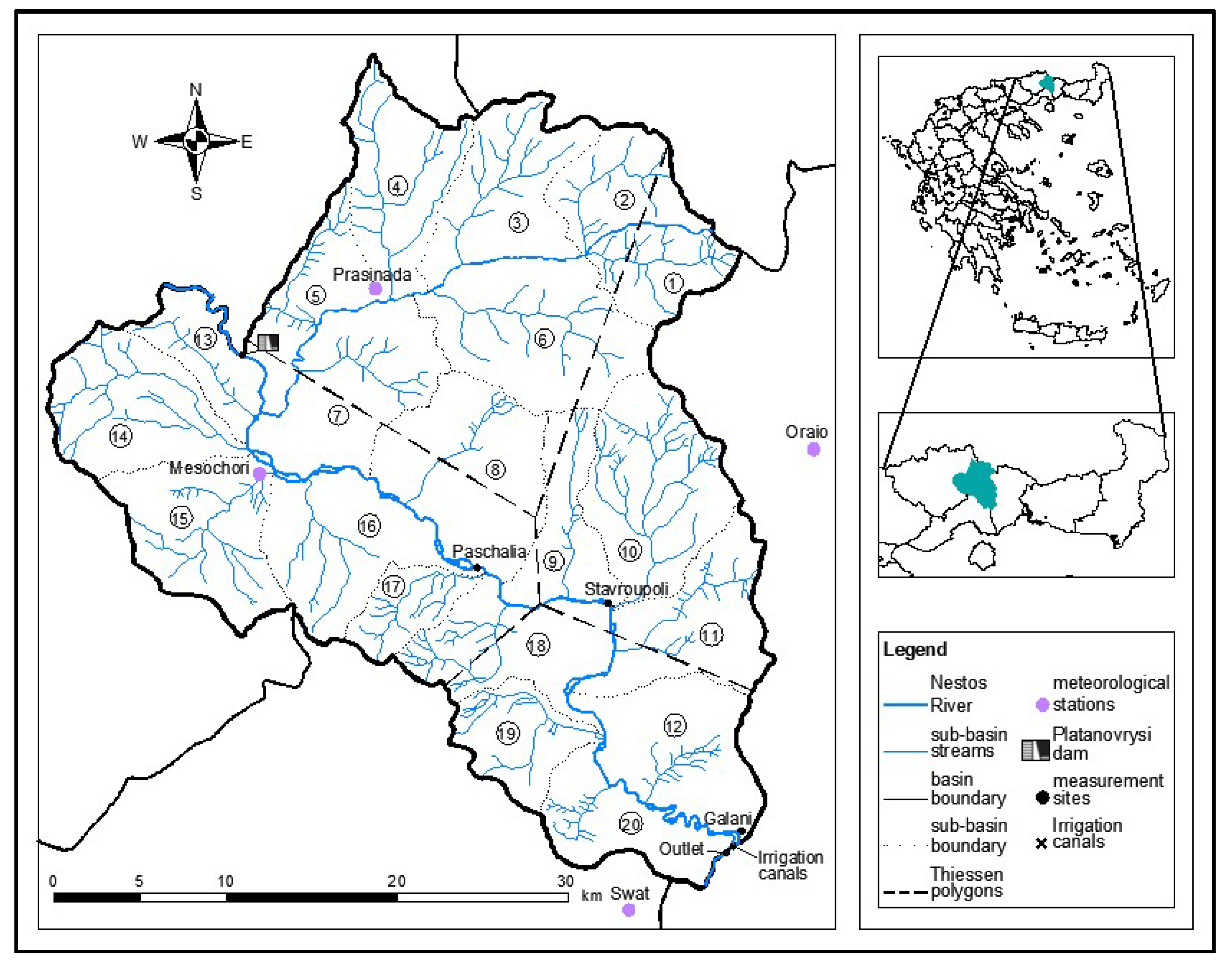
The under study part of Nestos River basin concerns the Greek mountainous part downstream of Platanovrysi dam (Figure 1). The basin extends to an area of 838.63 km², the altitude varies between 38 m and 1747 m, the average land slope of the basin is 37% and the length of the part of Nestos River that runs the basin, is approximately 63 km. The characteristic of the basin is the presence of a dam at its upper boundary, which greatly affects the discharge, as well as the sediment transport in Nestos River. Along with this, two irrigation canals slightly upstream of the basin outlet (Egnatia bridge of Nestos River) are responsible for the drastic reduction of water, during the irrigation period, disrupting the final discharge at the basin outlet. The four main soil types of the basin are: sandy clay loam, silty loam, loamy sand and silty clay loam. The basin is covered in its greatest part by forested and bushy areas and secondarily by crops, while a small fraction corresponds to urban areas and areas with no significant vegetation. There are four meteorological stations in the area of study: “Mesochori”, “Prasinada”, “Oraio” and “SWAT” (Figure 1). The distribution of the meteorological stations to areas of influence was achieved with Thiessen polygons [1] (Figure 1).

3. Materials and Methods

3.1. Theoretical Description of the IMM

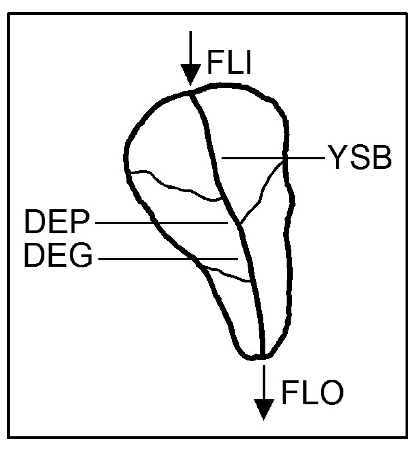
The basic computational concept of the present study consists in the application of the sediment continuity equation to the main stream of each sub–basin [2,3], as presented in Equation (1) and Figure 2:

$$FLO=FLI-DEP+DEG+YSB$$

(1)

where FLO is the sediment outflow from a sub–basin (t); FLI is the sediment inflow to the sub–basin (t); DEP is the sediment amount from FLI and YSB that is deposited on the bed of the sub–basin main stream (t); DEG is the sediment amount eroded from the bed of the sub–basin main stream (t); and YSB is the sediment yield due to soil erosion that reaches the sub–basin main stream (t).

3.1.1. Rainfall–Runoff Submodel

The rainfall–runoff submodel was built and simulated by the deterministic, semi–distributed hydrologic model HEC–HMS 4.2, and it consists of a combination of known methods:

• Hydrologic losses (mm) into the ground and rainfall excess—SCS–CN method [4]
• Evapotranspiration—FAO–56 Penman–Monteith method [5]
• Transformation of rainfall excess to runoff hydrograph—SCS unit hydrograph [6]
• Concentration time—Pasini’s formula [7]
• Baseflow—Exponential recession model [8]
• Routing of total discharge—Muskingum–Cunge model [9]

A much more thorough outline of the rainfall–runoff submodel can be found in [10,11].

3.1.2. Soil Erosion Submodel

The widely known Modified Universal Soil Loss Equation (MUSLE) [12] quantifies soil erosion caused by runoff as a function of six factors, according to Equation (2):

$$YSB=11.8·{\left(Q_{surf}·q_{peak}·area{}_{sub}\right)}^{0.56}·K·L·S·C·P$$

(2)

where YSB is the sediment yield, in t/h; Q_surf is the surface runoff volume (mm/km²); q_peak is the peak runoff rate (m³/s); area_sub is the area of the sub–basin (km²); K is the soil erodibility factor [t h/(MJ mm)]; L is the slope length factor; S is the slope steepness factor; C is the cover and management factor; and P is the support practice factor.

The parameters in the parenthesis, in Equation (2), refer to the runoff factor, introduced by Williams [12].

3.1.3. Streambed Deposition Submodel

Deposition (DEP) of sediment on streambed is modeled by means of the following relationships [13,14]:

$$D=100·\left(1-\frac{1}{e^x}\right)$$

(3)

$$x=\frac{1055·L·w}{u·h}$$

(4)

where D is the percentage of sediments (sand, silt, clay, gravel) that get deposited; L is the length of the reach (km); w is the fall velocity of sediment particles (m/s); u is the mean flow velocity (m/s); and h is the flow depth (m).

The fall velocity of sediment particles is calculated by the following formula:

$$w=\frac{1}{\mu }·\frac{D_{50}·\left({\rho }_s-\rho \right)·g}{18}$$

(5)

where μ is the dynamic viscosity of the water [kg/(s m)]; D₅₀ is the median particle diameter of the suspended sediment (m); ρ_s is the density of sediments (kg/m³); ρ is the density of water (kg/m³); and g is the acceleration of gravity (m/s²).

3.1.4. Streambed Erosion Submodel

The quantity DEG (t/h) is calculated by means of the formula of Smart and Jaeggi [15], who have improved the formula of Meyer–Peter and Müller [16] for bed load transport on the basis of laboratory experiments, in order to take into consideration greater bed slopes up to 20%.

$$DEG=Q_s·{\rho }_s·3600$$

(6)

$$Q_s=\frac{4.2·q·J^{0.6}·\left(J-J_0\right)}{p-1}$$

(7)

$$J_0=\frac{(p-1)·D_{50}}{20·h}$$

(8)

where Q_s is the volumetric sediment transport capacity (m³/s); ρ_s is the density of sediments (t/m³); q is the discharge (m³/s); J is the average slope of the main stream of each sub–basin; J₀ is the energy slope for flow without sediment transport; p is the fraction of the sediment density to the density of water; and D₅₀ is the median particle diameter of the bed load sediment (m).

4. Application, Calibration and Validation of the IMM

4.1. Model Application

HEC–HMS ran continuously from June 2008 to July 2014, resulting in runoff, baseflow and total stream discharge hydrographs (surface runoff + baseflow) at an hourly time step. All models ran continuously for the latter period and with the same time step. The runoff hydrographs, generated by HEC–HMS, trigger the processes of soil erosion, which is quantified by means of the MUSLE. More specifically, the sediment yields—due to soil erosion—that reach the main streams of the sub–basins are calculated. Subsequently, the amount of deposited sediments is calculated by means of the formulas of Einstein [13] and Pemberton and Lara [14], as a fraction of the sediment inflow to the sub–basin and the sediment yield due to soil erosion. The estimation of streambed erosion, by the formula of Smart and Jaeggi [15], concludes the determination of the sediment outflow from a sub–basin.

4.2. Model Calibration

An extensive calibration procedure was followed for all the submodels of the IMM. Starting from the rainfall–runoff submodel, a multi–site calibration procedure was implemented using the two upstream measurement sites, of Paschalia and Stavroupoli (Figure 1), for the calibration of the model, and the two downstream measurement sites, of Galani and the basin outlet, for the validation of it. A total of 81 discharge measurements were used for the calibration of the rainfall–runoff submodel (HEC–HMS). HEC–HMS was calibrated as to the four following parameters: Curve Number, lag time, baseflow recession constant, flow ratio. MUSLE was calibrated as to the following parameters: soil erodibility factor, slope length factor, slope steepness factor, cover and management factor, support practice factor. The calibration was carried out with the objective of lowering the initially high erosion rates calculated by the soil erosion submodel. The model for sediment deposition suffered a minor calibration, as to the flow depth, while the streambed erosion submodel was calibrated as to the median particle diameter, the discharge, the flow depth, and the slope of the main streams, with the last one being proven to be the most influential parameter for streambed erosion. The slopes of the main streams were slightly reduced during the calibration process. This was due to the main streams’ steepness, on account of the mountainous character of the basin, which led to relatively high streambed erosion rates.

4.3. Model Validation

HEC–HMS was validated at the measurement sites of Galani and the basin outlet, using 61 discharge measurements. A wide range of statistic efficiency criteria was used for the comparison between computed and measured discharge values.

34 sediment discharge measurements (bed load and suspended load), at the outlet of the basin, were used for the validation of MUSLE. Bed load measurements were accomplished by means of a net trap, while suspended load measurements were carried out by infiltrating a sample of water through a filter paper. A detailed description of the measurements’ procedure can be found in [17].

MUSLE, however, estimates the sediment yields—due to soil erosion—that reach the main streams of the sub–basins, and not the sediment discharge that finally reaches the outlets of the sub–basins. For the needs of routing of the amount of eroded soil that reaches the sub–basins’ main streams, MUSLE was coupled with a stream sediment transport submodel. The model of Yang and Stall [18] was used for the routing of sediments through the main streams of the sub–basins, in order to enable the estimation of sediment discharge at the outlet of the basin, on an hourly time step. Sediment transport capacity by streamflow is estimated from the sediment concentration in the stream, which is computed by the following relationship:

$$\begin{array}{cc}\hfill log{c}_{ts}=& 5.435-0.286log\frac{w{D}_{50}}{v}-0.457log\frac{u_{*}}{w}\hfill \\ \hfill & +\left(1.799-0.409log\frac{w{D}_{50}}{v}-0.314log\frac{u_{*}}{w}\right)log\left(\frac{us}{w}-\frac{u_{cr}s}{w}\right)\hfill \end{array}$$

(9)

where c_ts is the total sediment concentration by weight (ppm); D₅₀ is the median particle diameter (m); v is the kinematic viscosity of the water (m²/s); s is the energy slope; u_cr is the critical mean flow velocity (m/s); and u_* is the shear velocity (m/s).

The statistic efficiency criteria, used for the comparison between computed and measured values of water discharge and sediment discharge, provided satisfactory results for the rainfall–runoff submodel, on the one hand, and the soil erosion and stream sediment transport submodels, on the other hand (

Table 1. Efficiency criteria values for the validation of water and sediment discharge.

Efficiency Criteria	Galani Discharge	Basin Outlet Discharge	Basin Outlet Sediment Discharge
Mean absolute error (m3/s, kg/s)	2.933	2.494	0.160
Mean relative error (%)	13.188	25.466	45.076
RMSE (m3/s or kg/s)	4.426	3.866	0.276
Percent bias (%)	−15.491	−10.344	−5.927
Nash–Sutcliffe efficiency	0.650	0.974	0.903
Index of agreement	0.910	0.994	0.973
Correlation coefficient	0.894	0.992	0.953
Determination coefficient	0.800	0.985	0.908
t–test (p–value > 0.05)	0.192647385	0.67499631	0.865

).

Finally, an individual validation of the submodels for streambed deposition and erosion was not feasible, as streambed deposition and erosion measurements were not available. These submodels were validated in an indirect way through the final results of the IMM. At this point, it has to be noted that the objective of this study is the as possible accurate estimation of annual sediment yields, as a summation of hourly sediment yields. The computed annual sediment yield values, with the IMM, are compared with values that resulted from the implementation of two Composite Mathematical Models (CMMs) (

Table 2. Annual sediment yields at the basin outlet.

Year	Annual Sediment Yield (106 t/Year)			Annual Sediment Yield (t/km2/Year)
	Integrated Mathematical Model (IMM)	First CMM (Poesen)	Second CMM (MUSLE)	Integrated Mathematical Model (IMM)	First CMM (Poesen)	Second CMM (MUSLE)
2009	0.96	1.48	1.23	1147	1759	1470
2010	1.16	1.29	1.35	1382	1539	1611
2011	0.77	0.49	0.62	921	580	734
2012	1.43	1.40	1.12	1705	1664	1334
2013	1.35	1.10	1.10	1611	1308	1311

), each consisting of three submodels: a rainfall–runoff submodel (HEC–HMS 4.2), a soil erosion submodel and a sediment transport submodel for streams. The two models only differ in the soil erosion submodel. The first soil erosion submodel is based on the relationships of Poesen (1985) [19], while the second is MUSLE [12]. A comprehensive description regarding the application of the CMMs can be found in [20].

5. Results

In Table 1, the values of the efficiency criteria for the application of HEC–HMS (water discharge) and MUSLE–Yang and Stall (sediment discharge) at Galani and the basin outlet are displayed. The literature related to the efficiency criteria utilized in this study can be found in [10,20].

In Table 2, the annual sediment yields are given, for the entire basin and per km², for the period 2009–2013. In columns 3, 4 and 6, 7, the corresponding values of the two CMMs are provided.

As seen in Table 2, not only the values of the IMM are of the same order of magnitude with the values of the two CMMs, but there is an overall closeness between the results of the three models.

From the implementation of the IMM, it emerged that 100% of the available sediment that reaches the main streams, namely and , gets deposited. This is solely attributed to the high deposition rates, resulting from the relationships of Einstein [13] and Pemberton and Lara [14], which could not be counterbalanced by calibration. This is actually the reason for not applying an extensive calibration for the streambed deposition submodel. This practically means that the sediment outflow, , from each sub–basin is the sediment from streambed erosion, .

6. Discussion

In this study, an Integrated Mathematical Model (IMM) is applied at a continuous time scale in Nestos River basin. The IMM consists of a rainfall–runoff submodel, a soil erosion submodel, a streambed deposition submodel, and a streambed erosion submodel. The aim of the model is the calculation of sediment yields at highly disaggregated time steps. The structure and operation of the IMM is more than adequately described by Equation (1) and Figure 2.

Commonly, whether deposition or erosion takes place, in a stream, is defined on the basis of comparison between the available sediment in the stream and the sediment transport capacity by streamflow. If the available sediment in the main stream exceeds the sediment transport capacity by streamflow, deposition occurs, and the sediment yield is equal to sediment transport capacity. The other case is that the available sediment is less than the streamflow sediment transport capacity; this means that there is an energy excess which could be spent for bed detachment, and streambed erosion is very likely to occur. From a physical point of view, this rationale makes much sense. Paradigms of such applications are [10,20].

However, a much more different approach is attempted in this study, as the streambed deposition and the streambed erosion are modeled separately, regardless of the available sediment in the main streams and the streamflow sediment transport capacity. In other words, according to sediment continuity concept, both streambed deposition and streambed erosion may take place in a certain time period, whereas, according to the stream sediment transport concept, either streambed deposition or streambed erosion takes place in the time period considered. The latter concept seems to approach more the natural reality. Therefore, the comparison results between the measured and the computed sediment discharge at the basin outlet according to the former concept, on an hourly time basis, are not satisfactory.

The quantity refers mainly to suspended sediment that may be deposited. The quantity is transported in a stream as suspended load. However, the quantity may contain both bed load and suspended load.

The structure of the equations of Einstein [13] and Pemberton and Lara [14], shows that deposition should be investigated in very short stream segments and for relatively high flow depths and flow velocities, in order to provide reasonable results. This highlights the need for further investigation on streambed deposition and research for other streambed deposition models.

7. Conclusions

This study presents an efficient application of an IMM for the estimation of annual sediment yields, as a result of summation of hourly sediment yields. It is concluded that there is a very good approximation between the results of the IMM with the CMMs.

Despite its relatively simplistic logic, the IMM is a quite intricate model when it comes to its configuration and application. It is really an elaborate synthesis of models that reproduce the very complex hydromorphological processes which are triggered once rainfall starts. It goes without saying, that the synthesis of the IMM is adaptable and that individual submodels could be replaced with others, depending on the needs and characteristics of each study. This highlights the significance of the conceptualization presented rather than the case study itself.

The IMM can be efficiently used for the estimation of annual sediment yields. However, the results have shown that the IMM, after the inclusion of the streambed deposition and the streambed erosion submodels, lacks accuracy when applied at fine time steps, aiming at the simulation of hourly sediment yield values. However, its accuracy increases when the hourly sediment yields are summed in temporally lumped time steps (monthly, annually). This is because of the integrating effect obtained through the summation of hourly sediment yields for a long simulation period. In a nutshell, the IMM is recommended for the estimation of annual sediment yields.

The application of the IMM enables the calculation and the continuous assessment of sediment yields, at any desired point throughout a basin.