Pre-Localization Approach of Leaks on a Water Distribution Network by Optimization of the Hydraulic Model Using an Evolutionary Algorithm ^†

Abstract

The sustainable management of water distribution networks is a crucial challenge especially in emerging countries. The distribution networks have very low efficiency with very high levels of leaks. Locating and prioritizing of water leakage areas becomes a main concern for public services, to optimize the use of resources and improve constancy of supply. A decision support approach was proposed to locate areas with higher leakage rate. It is based on the resolution of the FAVAD equation (Fixed And Variable Area Discharge). The determination of FAVAD parameters enables to simulate the quantities and the location of the leaks, through the use of genetic algorithms coupled with hydraulic modeling and the geographical information system (GIS).

1. Introduction

One of the major challenges facing water utilities around the world is the high level of water losses in the distribution networks. In a World Bank study published by [1] estimated that more than 32 billion cubic meters of treated water are lost each year to fleeing urban water supply systems through the world and half of these losses occur in developing countries. According to the Water Operators Partnerships of the African Utility Performance Assessment published in (2009), Non-Revenue Water (NRW) have reached alarming levels in many developing cities, particularly in sub-Saharan Africa [2] Regarding the Algiers network, the Algerian Water and Sanitation Company (SEAAL) estimated in 2017 that the percentage of overall loss was 44%.

Leaks in water systems generally appear due to the aging of the infrastructure, generated or amplified by corrosion, or to mechanical constraints which are particularly exposed by the increase in operating pressure.

Many experimental researches have reported that the reduction of the pressure, induces the reduction of the leaks [3] without omitting those of [4] which showed that a reduction of the pressure of 77 m to 50 m resulted a reduction of 25% in MNF (minimum night flow).

The work carried out in this document boils down to proposing a methodology that aims at pre-locating leaks in a drinking water supply system using a model calibrated and built using the developed tool ExpaGIS. The application of the FAVAD concept is an appropriate solution for this kind of resolution.

Once the hydraulic model is constructed and calibrated flow rate through a simplified methodology, the use of Genetics Algorithms (GA) is required for the spatial distribution of leaks in the network nodes (model). To do this simulation we deployed a decision tool help ‘Optim_Detect’ programmed in the Matlab & interfaced with the hydraulic modeling tool through the EPANET toolkit.

Optim_Detect allows in fact the simulation of the parameters composing the concept of FAVAD (C_i and N1) in order to identify the quantity and the positioning of the leak on each nodes i of the hydraulic model. For a better representation of the results and system management, outputs are exported to a Geographic Information System (GIS).

In order to test and validate the proposed approach, many pilots were tested, where the total pipe length vary between 12 and 25 km, the results of these optimization were quite satisfactory. In this document an example of an important network (87 km) is presented. Through the use of the proposed tool and the measurements made in the field, 36 leaks have been pre-localized which represents a leakage rate of 57 m³/h, the discharge coefficients of the nodes obtained vary between 0.010 and 0.032, the emitter exponent N1 is simulated at 1.1.

2. Materials and Methods

2.1. Modeling the Behavior of the Leak in EPANET

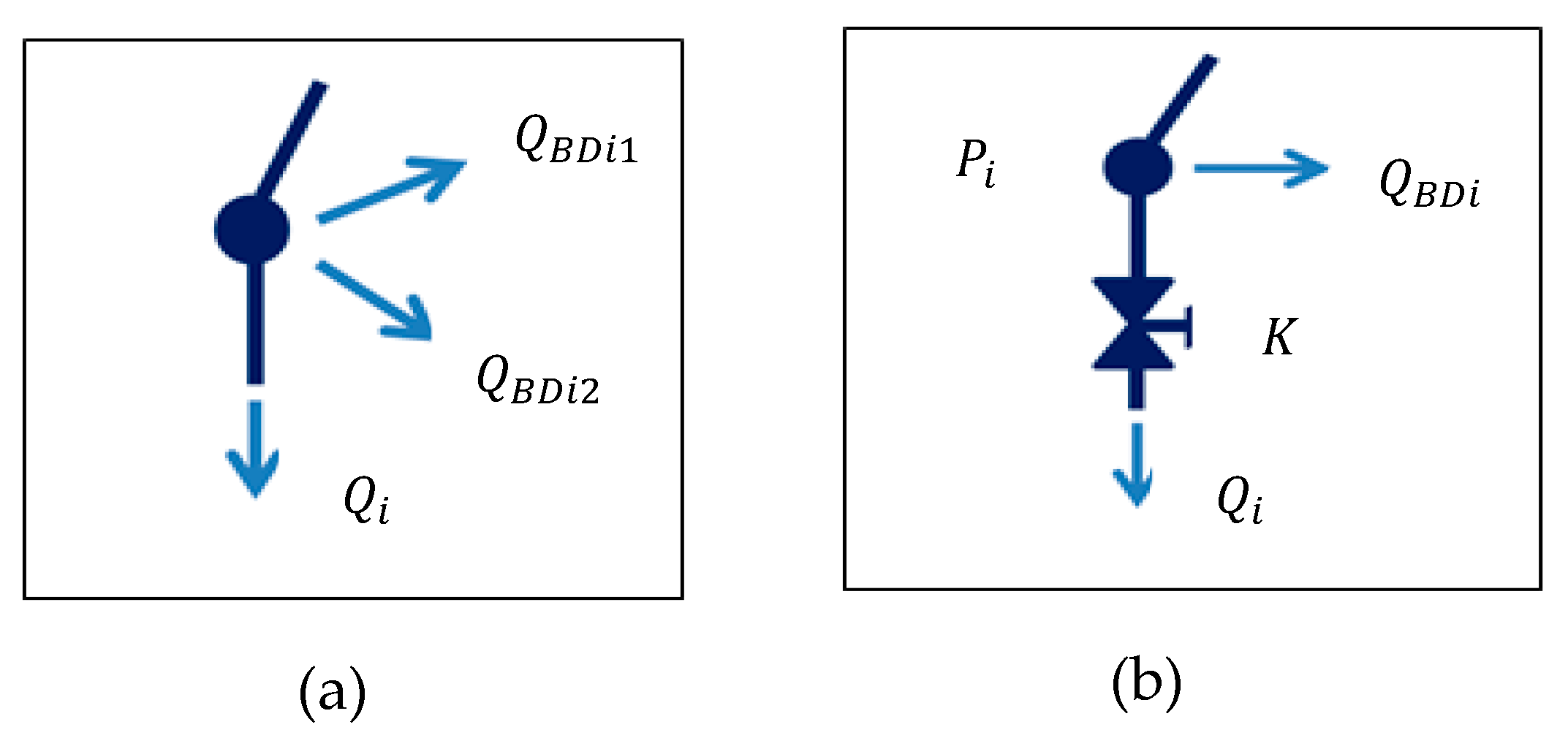
One of the main features of EPANET is that its hydraulic calculation engine is demand-driven. The water output data at each node is defined as the base demand. There are two ways to model a water leak in EPANET (Figure 1).

2.1.1. Method 1: The Leak Does Not Depend on the Pressure

The leak is modeled as an additional demand, independent of the pressure in a consumption node Figure 1a, in this case the formulation of the global flow of a node i is demonstrated in the Equation (1):

$$Q_i\left(t\right)=Q_{BDi1}\ast C_c\left(t\right)+Q_{BDi2}\ast C_l\left(t\right)$$

(1)

where $Q_{BDi 1}$ is the base demand for consumption, it is an average annual consumption of users based on individual meter indices. The customers are geo-located (knowing the x and y coordinates of each customer), their consumption is assigned to the nearest nodes in the hydraulic model by using the SIG/EPANET export tool (ExpaGIS). $Q_{BDi2}$ is the additional consumption of leakage, determined from the minimum night flow Q_MNF and homogeneously distributed to all nodes assuming that$: Q_{MNF}$ =${{\displaystyle \sum }}^{\text{}}{Q}_{BDi2}$ and the leakage time profile is constant $C_l$ =1 over the duration of the simulation (24 h) following a time step of 1 h. The consumption profile $C_c\left(t\right)$ is calculated by subtracting the minimum night flow rate Q_MNF from the measured hourly total flow rate.

2.1.2. Method 2: The Leak Depends on the Pressure (FAVAD Concept)

According to [5,6], the best way to represent leaks in a hydraulic network model is not through an additional demand, but rather with adding a leakage valve for each node i, as shown in Figure 1b.

Where $Q_{BDi}$ is the base node demand (consumption) got from the costumers’ indexes, P_i is the node pressure, K is the flow coefficient of the valve. It is depending of the change of the section and Q_i is the flow rate in the valve, representing the leakage. In this representation, the pressure at the node behaves as a determining factor of the leak, therefore the flow of a leak through the valve can be estimated.

2.2. Using the FAVAD Concept for Leak Pre-Locating

When simulating a leak in EPANET, the parameter that represents the coefficient of flow rate through a valve is the emitter. This emitter represents a valve open to the atmosphere it is a simple element of the node. The Equation (2) that represents the methodology mentioned above is the FAVAD concept:

$$Q_{Li}=C_i\ast P_i^{N1}$$

(2)

where $Q_{Li}$ is the leakage rate at node i, $C_i$ is the discharge (emitter) coefficient, $P_i^{ }$ is the simulated pressure at node i and N1 is the exponent emitter representative of entire network in EPANET, So the total flow of each node i is represented in Equation (3):

$$Q_i\left(t\right)total={\displaystyle \sum }_i^n[\left(Q_{BDi}\ast C_c\left(t\right)\right)+(C_i\ast P_i^{N1})]$$

(3)

The use of the equation above makes it possible to correctly represent the behavior of the leaks in a hydraulic model. The goal research is therefore the determination of the parameters C_i of each node of the hydraulic model and N1 representative of the whole network in order to be able to determine a leak rate specific to each node over a time t and to be able to pre-locate the leaks on a distribution network. According to the bibliography the exponent N1 = 0.5 for steel pipe, N1 > 1.2 for plastic pipe and N1 = 1 for other types of materials [6].

Table 1. Parameter determination (consumption and leakage).

Parameter	How to Determine the Parameter?	The Needs to Determine the Parameters
$Q_{BD i}$	Customers data.	Individual meter indices and geographical coordinates (x, y) of customers.
$C_c\left(t\right)$	Initial calibration of the model	Pressure and flow measurements
$P_i^{ }$	Result of the hydraulic modeling	Profile consumption
$C_i$	Optim_Detect tool	Genetics Algorithms GA
$N1$	Optim_Detect tool	Genetics Algorithms GA

summarizes the methodologies proposed in this document to determine the parameters of Equation (3).

2.3. Hydraulic Model Calibration Using FAVAD Concept

The determination of the initial consumption profile and the introduction of leaks in the hydraulic model is essential in order to launch a first optimization, the determination of this daily profile is possible by using a simplified methodology which is proposed in this document to distribute the leakage equitably over all network nodes. This methodology requires consideration of the following conditions:

• Use of a single emitter coefficient C_unique for all the nodes of the network; $C_1=C_2=C_3=\dots =C_n$.
• The emitter exponent N1 is considered equal to 0.5 according to the equation of the flow of an orifice through a fixed surface.
• ${\displaystyle \sum }_{i=1}^n{Q}_i$=$\overline{Q_{ obs}}$ according to the equation of mass conservation and continuity where; $Q_i$is the flow at a node i and $\overline{Q_{ obs}}$ is the observed average flow in the hydraulic model.

The simplified method used is presented below:

• Determination of the unique emitter coefficient for all nodes of the network by using the FAVAD concept; $C_{unique}=\frac{Q_{MNF}}{\sqrt{\overline{P{M}_{i MNF}}}}$; where $Q_{MNF}$ is Minimum Night Flow and $\overline{P{M}_{iMNF}}$ is the average pressure (During MNF) of the k pressure sensors installed in the network
• Using the unique emitter coefficient $C_{unique}$ for all the nodes in each time step to calculate of the hourly leakage rate $Q_{BDi 1}{C}_c\left(t\right)$ using the Equation (2) and deduce after the hourly leak profile$C_f\left(t\right)$
• Subtraction of the leak rate of the measured global flow to deduce the hourly global consumption $Q_{BDi 1}{C}_c\left(t\right)$.
• Verification of the consistency between the hourly total consumption and the meter data of the costumers. This allows the construction of the consumption profile$C_c\left(t\right)$.

2.4. Spatial Pre-Locating of Leaks Using Genetics Algorithms

Genetic algorithms are optimization algorithms based on the natural evolution theory of Darwin and Mendel’s work on genetics. They belong to the family of evolutionary algorithms that evolve the individuals of a population, initially chosen at random, by the application of the genetic operators. According to [7] a genetic algorithm is defined by:

• Individual/chromosome: a potential solution of the problem that corresponds to a coded value of the variable (or variables) in consideration;
• Population: a set of chromosomes or points in the search space (therefore coded values of variables);
• Environment: the research space (characterized in terms of performance corresponding to each possible individual);
• Fitness function: the function to optimize, it represents the adaptation of the individual to his environment.

2.4.1. Basic Concept of a Genetic Algorithm

A genetic algorithm aims to optimize a function defined on a search space. It must have the following five elements in order to be used:

• A coding principle of the population element. This step associates with each point of the state space a data structure. The quality of data coding conditions the success of genetic algorithms.
• A generating mechanism of the initial population. This mechanism must be capable of producing a non-homogeneous population of individuals that will serve as a basis for future generations.
• A function to optimize. This one returns a value called fitness or function of evaluation of the individual.
• Operators to diversify the population over generations and explore the state space.
• Sizing parameters: size of the population, total number of generations or stopping criteria, probabilities of application of crossover and mutation operators.

2.4.2. Problem Formulation by Genetic Algorithms

The use of (GA) in this document allows the optimized determination of the parameters of the FAVAD concept.

The fitness function at the end of the process allows to minimize the difference between the simulation results and the measured data transmitted from the exploitation of k sensors in the network. The minimization of the objective function f(x) can be obtained by minimizing the equation of the sum of the absolute differences following:

$$f\left(x\right)={\displaystyle \sum }_{j=1}^k\left|P_{obs j}-P_{sim j}\right|\le \epsilon$$

(4)

where the vector $\left[\begin{array}{c}{C}_i\\ N1\end{array}\right]$ of dimensions’ n + 1, is the chromosome consisting of the parameters of the concept of FAVAD, $P_{obs j }$and $P_{sim j }$ are respectively the observed and simulated pressures at the node k pressure sensors placed in the network. The formulation f(x) ≤ ε refers to the minimization principle of the objective function. The error threshold (ε) is defined as the minimum acceptable by the user. The evolution of the optimization process ensures that the following conditions are met:

• The constraint of the mass conservation (the incoming flow equals the outgoing flow):${\displaystyle \sum }_{i=1}^n{Q}_i$=$\overline{Q_{ obs}}$; Where every generation must respect this mass conservation constraint.
• The lower and upper bounds of the unknown parameters: $\underset{\_}{C_i}\le C_i\le \overline{C_i}$; Where$C_i$ $\in$ $\{0,1\}$ (Principle of flow through an orifice) and $\underset{\_}{N1}\le N1\le \overline{N_1}$ Where $N1 \in$ $\{0.5,2.5\}$, This emitter exponent may be equal to 0.5 for a leak that flows through a fixed surface orifice but may vary in real situations of leakage in the water networks in a range of 0.5 to 2.5 [8].

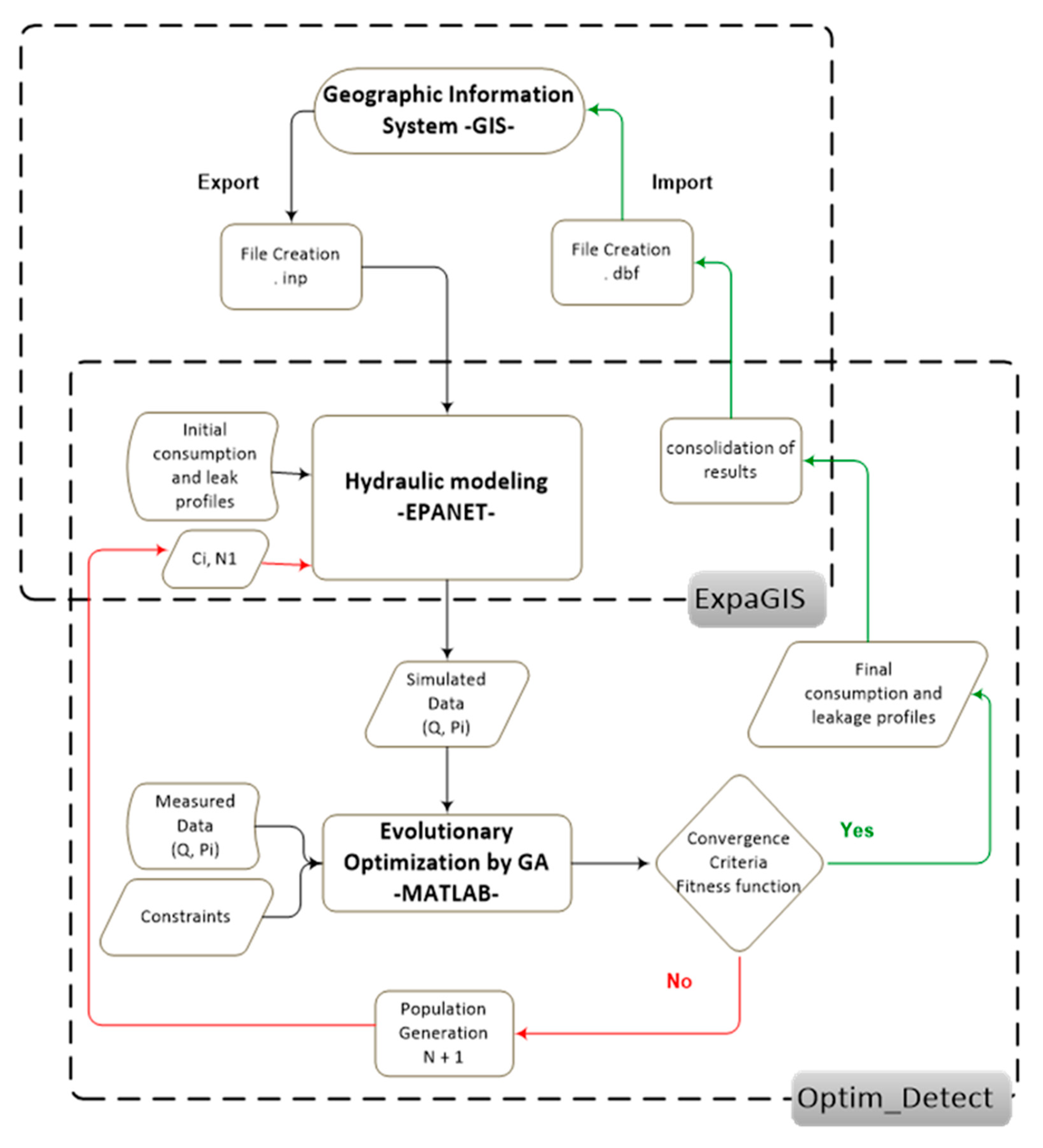
A decision support tool (Optim_Detect) has been developed for pre-locating leaks in Matlab in interface with EPANET and using the EPANET Toolkit’s dynamic link library (DLL) [9].

The input data for the tool for the calibration of the model are:

• A file (.inp) named from the hydraulic model concerned to its initial state (before calibration).
• Specification of the time that corresponds to the Minimum Night Flow (MNF), in order to calculate the quantities of leaks on each node at this time, before importing the data to the GIS for visualization of the results.
• Definition of GA parameters as (population size, generation number, number of elites, crossing rate ...) according to the user’s choice.

The output data are:

• A distribution of the transmitter coefficients in each node of the network and the allocation of a single exponent of the transmitter for the whole network, following the definition of the fitness function and the respect of the constraints.
• The evaluation of each population indicates two fundamental notions: “the Best fitness” which is the best Fitness (adjustment) obtained and “the mean fitness” which represents the average of the Fitness (adjustments) resulting where the achievement of the optimum occurs when (the mean fitness) converges to (the best fitness).
• The procedure summarizing the main phases of this process is presented in Figure 2:

3. Case Study

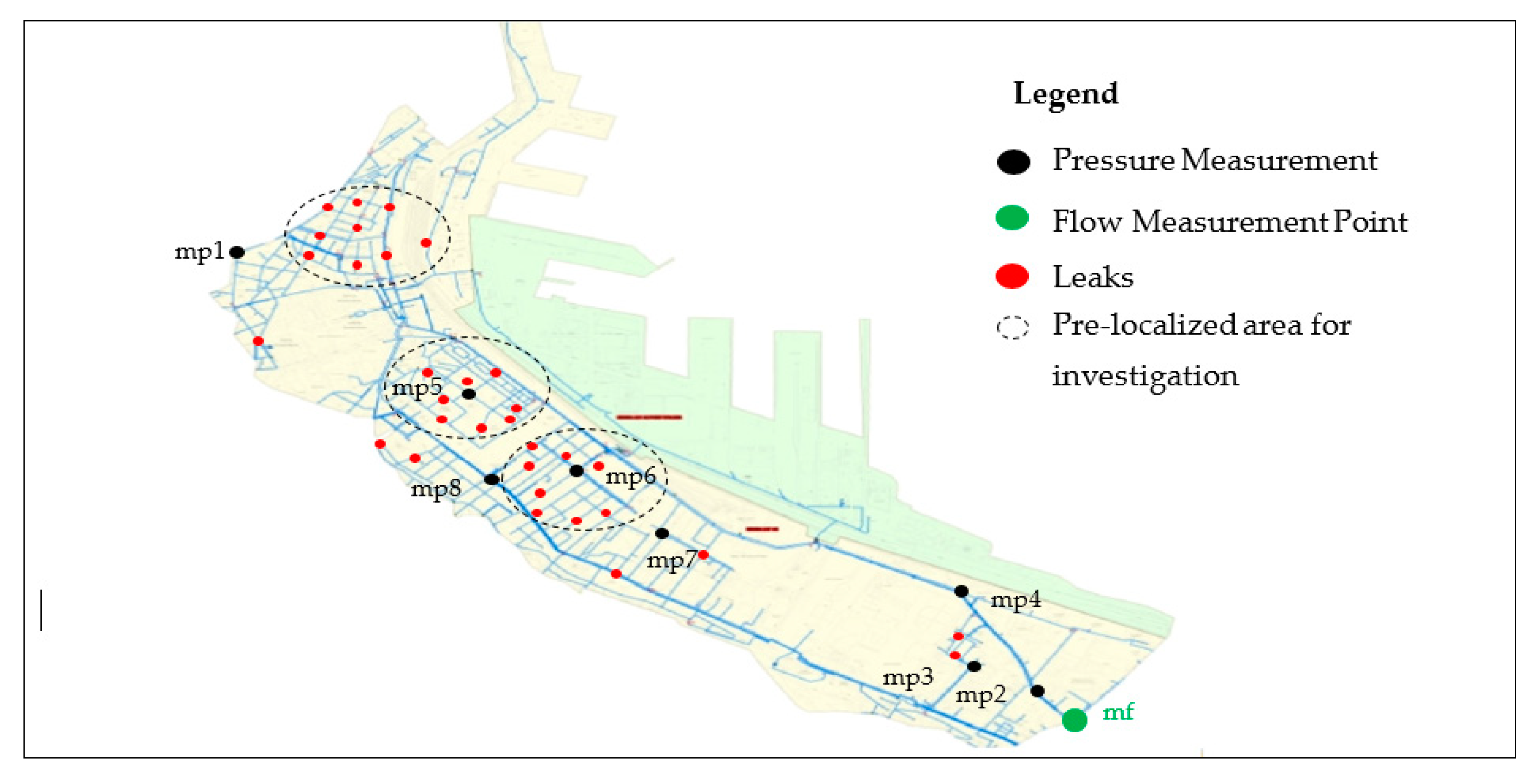
The study area K117 is located in the center of the capital of Algiers whose population is 90,000 inhabitants. The percentage of Non-Revenue Water (NRW) is equal to 47% with a linear loss index (LLI) of 140 m³/day/km. The network consists of 1380 pipes with a total length of 87 km, it has 1242 nodes. The diameters of pipes are between 80 and 800 mm, the network is controlled in pressure through a modulation valve in diameter 800 mm, this valve delivers the pressure according to the consumption profile. The main materials of this network are: galvanized steel, ductile iron and high density polyethylene. The network being composed of a multitude of materials. In the first approach the roughness is identical for all the arcs, it is estimated arbitrarily at 0.1 mm on average. This value is representative of the age and the structural state of the network. The roughness is not used as calibration parameter of the model in this study.

The K117 distribution network is composed of 8 sectors, each of these sectors is equipped with a (mpi) pressure sensor located in the center of the sector to improve representativeness, while adopting a secure location. At the entrance of the network, there is a control valve and a flowmeter (fm) where data is uploaded daily at 5-min intervals and archived in a Long-Term Database (LTBD) via a remote management and supervision system TOPKAPI.

4. Results and Discussions

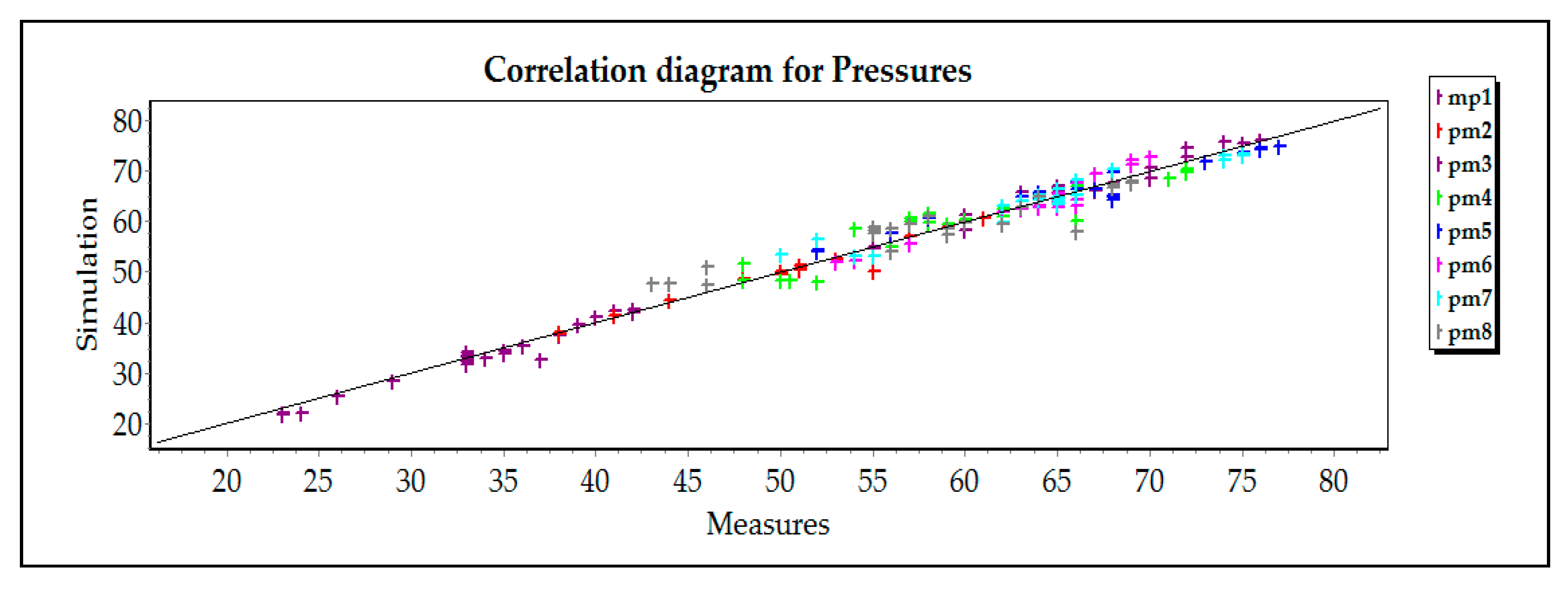
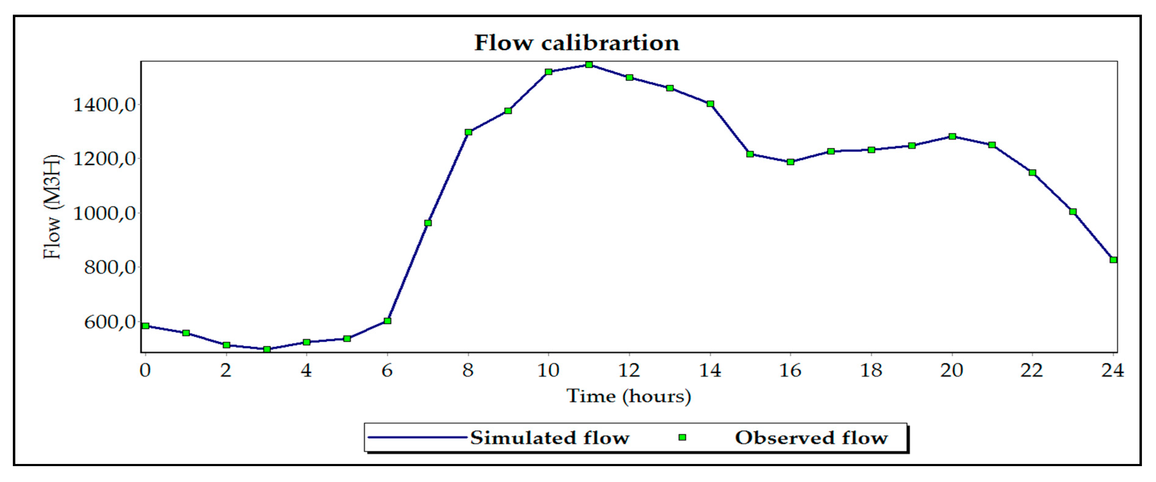
The calibration of the model (flow and pressure) was successfully carried out using the Optim_Detect tool. It was tested and validated by minimizing the fitness function, comparing the pressure and flow rate values measured with the results of the simulation.

During the calibration process, the coefficients C_i and the emitter exponent N1 were adjusted as calibration parameters of the flow rate and of the 8 points of pressure measurements. The calibration results are presented in Figure 3 and Figure 4.

The Optim_Detect tool simulates and distribute leakage coefficients (C_i) on each network node and simulation of the emitter exponent N1 by optimizing the Genetic Algorithms. The calculation of the magnitude of the leaks at the time corresponding to the (MNF) on each node of the network is done through the use of the Equation (2). After simulation, emitter coefficients Ci ∈ {0–0.032} and an emitter exponent N1 = 1.1. The use of 8 pressure measurements allowed the location of 36 real invisible leaks, these leaks are located at three areas and vary between [0.78–1.98] m³/h.

Figure 5 and

Table 2. Quantification of the leaks.

ID_Node	Pi (m)	Ci	QLi (m3/h)	ID_Node	Pi (m)	Ci	QLi (m3/h)	ID_Node	Pi (m)	Ci	QLi (m3/h)
605501	53.04	0.018	1.42	605431	56.2	0.018	1.51	604190	60.55	0.021	1.92
605510	55.62	0.015	1.25	608643	52.6	0.01	0.78	604188	62.51	0.017	1.61
608757	55.87	0.018	1.50	605494	54.3	0.022	1.78	604196	61.82	0.019	1.77
608186	49.02	0.022	1.59	605429	49.1	0.019	1.38	604209	60.5	0.02	1.82
608750	44.68	0.029	1.89	608731	52.7	0.018	1.41	604211	58.89	0.022	1.95
608691	46.8	0.028	1.92	605490	59.3	0.015	1.34	604197	61.02	0.016	1.47
605503	38.19	0.026	1.43	605424	55.9	0.022	1.84	604206	62.32	0.018	1.70
608697	40.2	0.027	1.57	605418	59	0.021	1.86	604202	61.66	0.019	1.77
605509	42.6	0.032	1.98	605418	52.3	0.012	0.93	604201	62.93	0.018	1.71
605509	38.9	0.017	0.95	605455	47.7	0.017	1.19	604200	62.18	0.019	1.79
318003	50.8	0.024	1.81	605512	49	0.016	1.16	608346	63.63	0.018	1.74
608355	63.07	0.02	1.91	608351	62.13	0.019	1.78	608352	62.37	0.017	1.60

respectively represent the results of the spatial distribution of leaks at the network nodes on a geographic information system (GIS) as well as the quantification of these leaks on each node of the network.

5. Conclusions

This work has developed a method for the continuous pre-location of leaks in a water supply network. The procedure was based on an optimization by Genetic Algorithm (GA) of the parameters of the FAVAD concept. The objective is to minimize the gap between the simulated and measured data. This optimization required an interface between a hydraulic model via a Genetic Algorithm (GA) and a Geographic Information System GIS. This approach can be applied in networks where NRW are very important. The calculation of these losses is done during the night period (2–4 h) where a minimum nighttime flow Q(t)_MNF is important and an excessive pressure allowing the suspicion of presence of leakage by the application of the FAVAD concept.

The Optim_Detect tool is proposed to target critical points of leakage, thus contributing to help utilities in their efforts to reduce physical losses. The identification does not always necessarily tip accurately on the location of the leak, but it significantly reduces the uncertainty and thus allows leak detection teams in the field to obtain better detection rates more quickly in areas where leaks have been pre-located.

References

- Kingdom, B.; Liemberger, R.; Marin, P. The Challenge of Reducing Non-Revenue Water (NRW) in Developing Countries. In The World Bank, Water Supply and Sanitation Sector Board Discussion Washington; Paper NO (08); World Bank Group: Washington, DC, USA, 2006. [Google Scholar]
- WSP. Water Operators Partnerships: African Utility Performance Assessment; Water and Sanitation Program, the World Bank: Nairobi, Kenya, 2009; Available online: http://documents.worldbank.org /curated/en/236571468209987559/pdf/508580WSP0WOP1Report0Box342008B01PUBLIC1.pdf (accessed on 19 April 2017).
- Babel, M.S.; Islam, M.S.; Gupta, A.D. Leakage Management in a low-pressure water distribution network of Bangkok. Water Sci. Technol. Water Supply 2009, 9, 141–147. [Google Scholar] [CrossRef]
- Marunga, A.; Hoko, Z.; Kaseke, E. Pressure management as a leakage reduction and water demand management tool: The case of the City of Mutare, Zimbabwe. Phys. Chem. Earth 2006, 31, 763–770. Available online: www.sciencedirect.com (accessed on 22 April 2017). [CrossRef]
- Al-Ghamdi, A.S. Leakage–pressure Relationship and leakage detection in intermittent water distribution systems. J. Water Supply Res. Technol. Aqua 2011, 60, 178–183. [Google Scholar] [CrossRef]
- Cobacho, R.; Arregui, F.; Soriano, J.; Cabrera, E., Jr. Including leakage in network models: An application to calibrate leak valves in EPANET. J. Water Supply Res. Technol. Aqua 2014, 64, 30. [Google Scholar] [CrossRef]
- Lerman, I.; Ngouenet, F. Algorithmes génétiques séquentiels et parallèles pour une représentation affine des proximités; INRIA: Rennes, France, 1995. [Google Scholar]
- Tabesh, M.; Asadiyani Yekta, A.H.; Burrows, R. An Integrated Model to Evaluate Losses in Water Distribution Systems. Water Resour. Manag. 2009, 23, 477–492. [Google Scholar] [CrossRef]
- EPA EPANET. Model for Water Distribution Piping Systems. Available online: http://www.epa.gov/ nrmrl/wswrd/dw/epanet.html (accessed on 7 March 2014).