Identification of Annual Water Demand Patterns in the City of Naples ^†

Abstract

In the present paper, different clustering techniques were applied to detect significant patterns describing single-household water consumption in a residential neighborhood of the City of Naples, basing on hourly time series aggregated at the monthly scale. Comparisons among results were performed by means of a selection of Clustering Validity Indices, that were adjusted to overcome a bias caused by sparsely populated clusters. The most performant cluster solution proved to be the one resulting from the application of a mixed strategy, namely a Self-Organized Map followed by K-means performed on first level cluster centroids.

1. Introduction

Water demand modeling and forecast is a key issue in modern approaches to an efficient water management. A comprehensive knowledge of water consumption allows for a correct planning of water supply, for the estimate of leakages in the water distribution networks and for the development of innovative approaches and attractive plans to consumers.

The increasing interest towards water systems efficiency has led to the implementation of “Smart Water Grids” within urban areas, with significant portions of customers connected to a telemetry system for flow data reading and collection. Smart grids allow for the collection of large amounts of data, usually on an hourly basis or less [1] that water companies can utilize to calibrate bills on the short term, and to perform research to increase efficiency on the long term. Understanding consumption drivers at the customer scale can be a challenging task in a complex urban environment because of the extreme variability in the characteristics of households, such as the number of individuals served by each flow meter, water usage (which can be related to either residential or commercial activities), different life habits of the end users. One common approach to solve this problem is the profiling, namely a detection of demand patterns based on a large amount of data; this is a typical approach in the electricity sector [2,3,4,5,6], with a few applications for water demand modeling [7,8]. Profiling of consumption data is typically performed to catch differences in the customers behavior, with particular focus on the weekdays/weekends distinction, especially when no previous information is known.

2. Materials and Methods

2.1. Data Description

The District Metering Area (DMA) which is the subject of the study is located in the North-Western part of the City of Naples (Italy). This area was chosen as a pilot area for a Smart Water Grid implementation, with particular focus on the remote monitoring of flow meters, as part of a cooperation between the University of Naples and ABC—Napoli, which is the local water company. The DMA is provided with 4254 customer connections whose flow meters were completely replaced during the last three years. There are 3701 (87% of the total number) residential flow meters, whereas the remaining 553 (13%) correspond to commercial flow meters, consistently with the residential purpose of the neighborhood. Moreover, 2999 (81% of the residential flow meters) connections relate to single households, whereas the remaining 702 (19%) flow meters serve multiple households, such as duplexes or whole apartment buildings.

The present paper focuses on single-household flow meters; for each flow meter 12 months of hourly consumption measurements are available, dating 1 January 2016 to 31 December 2016. After a data cleansing process, which caused the elimination of a certain number of time series, data were standardized and aggregated at the monthly scale:

$$Y_i=\frac{N}{M}·\frac{{{\displaystyle \sum }}_{j=1}^M{X}_j}{{{\displaystyle \sum }}_{k=1}^N{X}_k} i=1\dots 12$$

(1)

where Y_i is the standardized monthly data, N is the number of hourly data X_k contained in one year (N = 8784) and M is the number of hourly data X_j contained in one month. Furthermore, the analysis is limited to a selection of 168 single-household time series randomly chosen within the initial dataset. In future research, clustering results will be extended to the remaining time series by means of a supervised classification.

2.2. Clustering

Clustering is a data mining technique that consists in dividing an initial set of multidimensional data in different meaningful subsets containing objects that share similar characteristics, with the aim of discovering hidden recurring patterns [5,9]. An efficient clustering provides a number of final clusters such that the distance among data belonging to different clusters (usually referred to as “between-clusters distance”) is maximized, whereas the distance among data belonging to the same clusters (“within-clusters distance”) is minimized [3,7]. Given a couple of multidimensional data ${\overline{x}}_i$ and ${\overline{x}}_j$, the most common definition of their reciprocal distance $d\left({\overline{x}}_i,{\overline{x}}_j\right)$ is the Euclidean norm [10]:

$$d\left({\overline{x}}_i,{\overline{x}}_j\right)=\sqrt{\left({\overline{x}}_i-{\overline{x}}_j\right)·{\left({\overline{x}}_i-{\overline{x}}_j\right)}^T}$$

(2)

However, a large number of alternative distance metrics are available, including cosine distance, Mahalanobis distance, cosine wavelets and piecewise probabilistic measures among others [11,12,13,14].

A common classification of clustering techniques based on the clustering criterion is among “partitioning” or “non-hierarchical” methods (i.e., K-means), “hierarchical” methods (i.e., dendrogram) and “model-based” methods (i.e., Self-Organizing Maps) [5]. K-means is a clustering algorithm consisting in the crisp partition of multidimensional data into K subsets, with the number of clusters K defined by the user prior to the analysis [15]. The partition is made assigning each data to the nearest cluster center, or “centroid”; initial cluster centroids are assigned randomly and any available distance metric can be used. A number of iterations must be run in order to minimize the effect of the initial cluster centroids choice [5].

The dendrogram method consists in a bottom-up agglomeration of data based on reciprocal distance [16]. Starting from a condition where each data is a separate cluster, pairwise distances are computed and the two nearest data are merged into a new cluster, whose centroid is evaluated and pairwise distances are updated. The merging of couples of clusters continues until the desired number of clusters, which is defined by the user prior to the analysis, is achieved [5,17].

Self-Organizing Map (SOM) is an unsupervised clustering technique based on neural networks [18]. The main concept is that an input layer made up of initial data must be reduced in size and connected to an output layer by means of network parameters and adjustable weights [19]. The output layer usually consists of a bidimensional grid made up of a number K of typically hexagonal elements, or “output neurons”, which represent the maximum possible number of clusters, defined by the user prior to the analysis. SOM is also known as “topology feature preserving map” because the algorithm preserves data topology; in other words, close neurons in the output layer have similar characteristics because they were generated by similar input data [19,20]. The final output of SOM is represented by the output neuron grid, where each neuron can be empty, if no input data was found to be related to it, or filled with one or more input data, so that each neuron can be regarded to as a separate cluster. However, the in-deep insight of SOM results, implying visual inspection of neighboring distances and component planes, also taking additional information such as data labels into account [20,21], can lead to a merging of the nearest neurons with the consequent reduction of clusters.

There is no confirmation in literature about which is the most performant clustering algorithm, since each method has both advantages and drawbacks [2,3,5]. However, different methods are usually coupled with specific applications. As concerns smart metering data, several examples exist that adopt SOM clustering for energy consumption data to recognize multiple consumers typologies or to discriminate weekdays from weekends consumption [2,6,20]. In the field of water consumption pattern analysis, recent applications include K-means [7] and SOM [21]. Dendrogram applications are rare, since this method implies a deep computational effort to compute the dissimilarity matrix when the initial dataset is large [22].

Whichever the algorithm used for clustering, one key parameter is the number of clusters K (or its equivalent for SOM, namely the output grid dimension). In practical applications, some prior information is usually available so that the choice of K is data-driven and not arbitrary (for instance, when using K-means the number of consumers typologies could be known). As concerns SOM, the choice of the output grid dimension (which is the square root of the maximum allowed number of neurons) can follow two different strategies. The first approach consists in setting a very large output dimension in order to obtain an output map made up of groups of neurons occupied by one or few data, delimited by groups of empty neurons. This method is usually applied when there is a prior knowledge about data labeling (for example the corresponding day of the week is known) and the merging of close neurons into clusters is straightforward. At the opposite, when no prior information or labeling is available, it is more useful to set a small grid dimension and let each neuron be hit by a considerable number of data. When this happens, the output neurons coincide with the final clusters, although a posterior merging of the nearest neurons can always be considered.

In general, when prior knowledge is little or absent, it is a common practice to repeat computations with different values of K and compare results, looking for the best “cluster solution” in terms of clustering quality. The performance of a cluster solution can be evaluated by means of the Clustering Validity Indices (CVIs). A large number of CVIs has been proposed in literature [2,23] and there is no general consensus about which should be the most useful [5]. A general approach is to pick the cluster solution that either minimizes/maximizes a certain CVI or corresponds to an elbow/local peak of the function [23]. However, it is important to understand that taking more than one CVI into account at the same time could lead to problematic clustering evaluation, because multiple CVIs seldom give the same results; the choice of which CVI to use and the interpretation of results should be considered heuristic [23].

Among all the proposed CVIs the most frequently used are based on the definition of between-clusters distance SSB and within-clusters distance SSW, which account for the definition of distance proposed in Equation (2):

$$SSB={\displaystyle \sum }_{k=1}^K{n}_k·d^2\left({\overline{C}}_k,\overline{M}\right)$$

(3)

$$SSW={\displaystyle \sum }_{k=1}^K{\displaystyle \sum }_{i=1}^{n_k}{d}^2\left({\overline{x}}_i,{\overline{C}}_k\right)$$

(4)

where n_k is the number of data in cluster k, ${\overline{C}}_k$ is the centroid of cluster k and $\overline{M}$ is the mean of all data in the dataset. In other words, SSB is defined as the sum of square distances of the centroids of each cluster from the mean, weighed by the size of each cluster. For the evaluation of SSW, for each cluster the square distance of all data belonging to that cluster from the cluster centroid must be computed, and their sum is computed for all the clusters in the cluster solution. Whichever the algorithm adopted and the initial dataset, by definition SSW increases and SSB decreases for increasing K, and their sum remains constant [3]. SSB and SSW can be used in combination with other CVIs or even alone to make some preliminary cluster evaluation: for example, the best cluster number K could be chosen as that value where SSB and SSW stabilize to an asymptote [2].

Basing on Equations (3) and (4), two CVIs were proposed that are the most frequently used for clustering evaluation, namely the Calinski-Harabasz index CH and the Davies-Bouldin Index DBI [24,25]:

$$CH=\frac{SSB}{SSW}·\frac{N-K}{K-1}$$

(5)

where N is the number of data in the initial dataset, and

$$DBI=\frac{1}{K}·{\displaystyle \sum }_{k=1}^{K}max\left(R_{kj}\right)$$

(6)

with:

$$\begin{gathered} R_{kj}=\frac{{\overline{d}}_k+{\overline{d}}_j}{d\left({\overline{C}}_k,{\overline{C}}_j\right)} \forall k,j\in K \\ {\overline{d}}_k=\frac{1}{n_k}·{\displaystyle \sum }_{i=1}^{n_k}d\left({\overline{x}}_i,{\overline{C}}_k\right) \end{gathered}$$

(7)

Computation of CH is straightforward once SSB and SSW have been calculated, whereas for the computation of DBI some successive steps must be accomplished. First of all, for each cluster k in the cluster solution the mean ${\overline{d}}_k$ (“average within distance”) of all distances of data in the cluster from the cluster centroid must be computed. Then, for each pair of clusters in the cluster solution the quantity R_kj must be computed which is the sum of average within distances of the clusters in the pair, normalized by the distance between the two centers. Finally, for each cluster k the maximum of R_kj is found, and DBI is the average of maximum R_kj values. The best cluster solution is the one that minimizes DBI or maximizes CH.

As seen, the state of the art related to clustering provides different techniques, along with different approaches to set relevant parameters and performance criteria, and there is no algorithm nor CVI performing suitably well in every context. For this reason, in the present paper a “mixed clustering strategy” was adopted that consists in combining different techniques to detect clusters in very large datasets, where single methods could perform poorly [26,27,28]. Specifically, a base partitioning was obtained with a first-level clustering by SOM, and a second-level clustering was performed to the centroids of the first-level clusters. For first-level clustering different output grid dimension values were tested, whereas for second-level clustering both K-means and dendrogram were applied with different cluster numbers K. Clustering performances were compared by means of DBI and CH indices.

3. Discussion of Results

No preliminary information is available that suggests a possible reliable cluster number K, nor literature points towards a specific clustering technique. As a consequence, different methods were applied and results were compared to find the optimal cluster solution. The in-depth analysis of cluster solutions required the estimation of several CVIs (CH and DBI were chosen) which, as stated in the previous sections, must be considered as a heuristic decision tool to be supported by additional observations about clusters consistency and meaningfulness.

Different models were applied to perform clustering, labeled model “A”, model “B” and models “C”. Model A and model B consist in the application of two ordinary techniques, namely K-means and dendrogram respectively, to the dataset made up of 168 monthly-aggregated normalized time series. For both models the algorithm was run with 27 different cluster numbers (henceforth called K₂) chosen in the range 2–64. Models C consist in a mixed strategy made up of a first-level clustering by SOM (with output grid dimension identified by the first number following letter “C”) and a second-level clustering by K-means (second number following letter “C” is 1) or dendrogram (second number following letter “C” is 2). For models C, SOM was run with 5 different output grid dimension $\sqrt{K_1}$ ranging between 4 and 8, where K₁ is the number of clusters of the 1st-level clustering. However, it must be noted that for high K₁ values not all the neurons could be occupied (for instance in models C81 and C82 the largest cluster solution is K₁ = 63 because one neuron was found empty), so that K₁ should be interpreted as the maximum possible number of clusters. As 2nd-level clustering, both K-means and dendrogram were run with K₂ ranging between 2 and K₁-1 with unit pace. To better understand the proposed procedure, the main points are summarized with a reference to a fictional model C_ad:

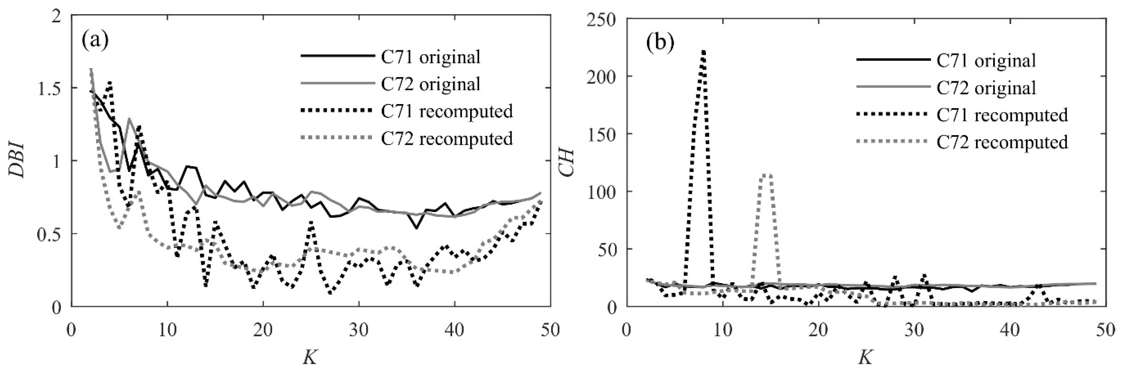
• As 1st-level clustering, a SOM is run with grid dimension set to a, so that the maximum allowed number of clusters is a². To minimize random errors, SOM is run 10 times and the best result is chosen as the one that minimizes the sum of distances data/cluster centroid. For each cluster, the centroid is computed as the mean of all the patterns in the cluster.
• As 2nd-level clustering, another clustering method (K-means for d = 1, dendrogram if d = 2) is run where the a² centroids are used as the input and K₂ is set to a value b ranging between 2 and a²-1. K-means is run 10 times with K₂ = b and for each run the algorithm replicates are set to 1000, in order to reach convergence and minimize the influence of initial points (same parameters were used for model A). Again, the best result is chosen as the one that minimizes the sum of distances data/cluster centroid. If the dendrogram is used, K₂ is set to b and there is no need to iterate computations, since the method is only based on initial distances.
• Finally, the original 168 patterns that were used as the input for 1st-level clustering are reassigned to the b new clusters, and DBI and CH can be computed with reference to the final partition, called “cluster solution”.

Comparison of models A and B shows that model B is preferable since it has the lowest DBI and the highest CH for each cluster solution; however, models A and B perform poorly if compared to models C. As concerns models C, results are conflicting since DBI and CH not only provide for opposite results in terms of K, but also the best cluster solutions systematically coincide with the highest or lowest possible cluster numbers, implying that the estimate of the CVIs is somehow biased. This circumstance can be explained observing that in the 1st-level clustering provided by SOM each cluster solution is made up of a small number of highly populated clusters and a large number of highly compact clusters containing a very small number of time series. Such a heterogeneity could distort the evaluation of the proposed indices.

In order to overcome such a bias and to extract useful information from CVIs inspection, for each cluster solution provided by the mixed-strategy models only the clusters containing more than 5 patterns were considered and DBI and CH were recomputed. Figure 1 shows original and recomputed CVIs for models C71 and C72 as an example; considerations are similar for all the other models. It must be noted that for original CVIs K coincides with the number of clusters in the cluster solution, whereas for recomputed CVIs K must only be interpreted as a label for comparison purposes, and the actual number of clusters can be lower than or equal to K. As concerns DBI (Figure 1a), recomputed values provide an optimal solution which is far more acceptable than the one provided by original DBI, since K is now intermediate with respect to the extreme values. Moreover, the new optimal solution has a lower DBI value, because neglecting sparsely populated clusters emphasizes the meaningfulness of the remaining ones. Recomputed CH values (Figure 1b) provide solutions that are now coherent with those provided by the recomputed DBI; also, CH is now characterized by pronounced spikes highlighting clustering solutions that are significantly meaningful than the others.

A visual inspection of the best cluster solution for each model suggests that the optimal cluster solution is K = 31 for model C71, which is characterized by 5 clusters containing more than 5 patterns. This solution is a relative maximum of recomputed CH (the absolute maximum values having an inconsistent number of meaningful clusters) and at the same time it corresponds to a recomputed DBI value which is very close to the minimum. Also, recomputed CH and DBI for this particular solution are among the maximum and minimum values, respectively, among all the solutions provided by the different tested models. Once the optimal solution was found, the 26 sparsely populated clusters were manipulated and suitably merged, reducing their number to 19 (5 highly populated plus 14 sparsely populated clusters).

Figure 2 shows the clusters of the optimal cluster solution, along with cluster centroids. Clusters 1–5 have more than 5 pattern each, and they can be considered meaningful because they have correctly detected different customers behaviors especially related to summer consumption. Specifically, cluster 2 shows a consumption increase in August, presumably related to customers that spent summer 2016 in town; clusters 1, 4, 3 and 5 show a progressive decrease consumption in August (this could be related to an increasing number of summer holidays with zero or low consumption). In all the other months of the year, however, clusters 1–5 show a similar behavior, with a water consumption that is quite constant. Clusters 6–10 can be considered meaningful as well since they have detected anomalous behaviors probably caused by instrumental problems; alternatively, they can be considered representative of households which were not occupied for large periods of the year. Clusters 11–19 are singleton clusters; such patterns were not assigned to any of the other clusters since their Euclidean distance from any of the centroids was larger than the average within distance in Equation (7).

4. Conclusions

In the present paper a procedure is presented to detect water consumption patterns describing significant consumers behaviours. The methodology presents some novelty elements. The adoption of SOM, although frequent in the framework of electrical consumption, is very rare for water demand problems. Moreover, the case study represents a useful example of mixed clustering strategy; the final partitioning stems from an in-deep analysis of clustering parameters that, apparently, provide for contradictory information whose interpretation is not straightforward.

The research was strongly supported by the local water company, who provided for water consumption data, because of the high potentialities of results for both research and management purposes. Detected patterns will be of great aid in inferring about non-monitored connections; this will allow for: (i) a more realistic calibration of bills; (ii) the efficiency increase on the long term; (iii) the evaluation of water balance in the WDN and, as a consequence, the estimation of leakage volumes; (iv) the evaluation of the outputs at significant spatial scales, such as the census scale, with the aim of seeking correlations with socio-demographic parameters.

References

1. Gargano, R.; Tricarico, C.; Del Giudice, G.; Granata, F. A stochastic model for daily residential water demand. Water Sci. Technol. Water Supply 2016, 16, 1753–1767. [Google Scholar] [CrossRef]
2. Rasanen, T.; Voukantsis, D.; Niska, H.; Karatzas, K.; Kolehmainen, M. Data-based method for creating electricity use load profiles using large amount of customer-specific hourly measured electricity use data. Appl. Energy 2010, 87, 3538–3545. [Google Scholar] [CrossRef]
3. Lopez, J.J.; Aguado, J.A.; Martín, F.; Munoz, F.; Rodríguez, A.; Ruiz, J.E. Hopfield-K-Means clustering algorithm: A proposal for the segmentation of electricity customers. Electr. Power Syst. Res. 2011, 81, 716–724. [Google Scholar] [CrossRef]
4. Ferreira, A.M.S.; Cavalcante, C.A.M.T.; Fontes, C.H.O.; Marambio, J.E.S. A new method for pattern recognition in load profiles to support decision-making in the management of the electric sector. Electr. Power Energy Syst. 2013, 53, 821–831. [Google Scholar] [CrossRef]
5. Zhou, K.; Yang, S.; Shen, C. A review of electric load classification in smart grid environment. Renew. Sustain. Energy Rev. 2013, 24, 103–110. [Google Scholar] [CrossRef]
6. Macedo, M.N.Q.; de Almeida, G.J.J.M.; de Lima, A.C. Demand side management using artificial neural networks in a smart grid environment. Renew. Sustain. Energy Rev. 2015, 41, 128–133. [Google Scholar] [CrossRef]
7. Avni, N.; Fishbain, B.; Shamir, U. Water consumption patterns as a basis for water demand modeling. Water Resour. Res. 2015, 51, 8165–8181. [Google Scholar] [CrossRef]
8. McKenna, S.A.; Fusco, F.; Eck, B.J. Water demand pattern classification from smart meter data. Procedia Eng. 2014, 70, 1121–1130. [Google Scholar] [CrossRef]
9. Sancho-Asensio, A.; Navarro, J.; Arrieta-Salinas, I.; Armendáriz-Íñigo, J.E.; Jiménez-Ruano, V.; Zaballos, A.; Golobardes, E. Improving data partition schemes in Smart Grids via clustering data streams. Expert Syst. Appl. 2014, 41, 5832–5842. [Google Scholar] [CrossRef]
10. Keogh, E.; Chakrabarti, K.; Pazzani, M.J.; Mehrotra, S. Locally adaptive dimensionality reduction for indexing large time series databases. ACM Sigmod Rec. 2001, 30, 151–162. [Google Scholar] [CrossRef]
11. Yiakopoulos, C.T.; Gryllias, K.C.; Antoniadis, I.A. Rolling element bearing fault detection in industrial environments based on a K-means clustering approach. Expert Syst. Appl. 2011, 38, 2888–2911. [Google Scholar] [CrossRef]
12. Benaichouche, A.N.; Oulhadj, H.; Siarry, P. Improved spatial fuzzy c-means clustering for image segmentation using PSO initialization, Mahalanobis distance and post-segmentation correction. Digit. Signal Process. 2013, 23, 1390–1400. [Google Scholar] [CrossRef]
13. Huhtala, Y.; Karkkainen, J.; Toivonen, H. Mining for similarities in aligned time series using wavelets. In Data Mining and Knowledge Discovery: Theory, Tools, and Technology; SPIE Proceedings Series; SPIE: Orlando, FL, USA, 1999; Volume 3695, pp. 150–160. [Google Scholar]
14. Keogh, E.; Smyth, P. A probabilistic approach to fast pattern matching in time series databases. In Proceedings of the 3rd International Conference on Knowledge Discovery and Data-Mining, Newport Beach, CA, USA, 14–17 August 1997; pp. 20–24. [Google Scholar]
15. MacQueen, J. Some methods for classification and analysis of multivariate observations. In Proceedings of the 5th Berkeley Symposium on Mathematical Statistics and Probability, Berkeley, CA, USA, 21 June–18 July 1965. [Google Scholar]
16. Johnson, J.C. Hierarchical clustering schemes. Psychometrika 1967, 32, 241–254. [Google Scholar] [CrossRef]
17. Jota, P.R.S.; Silva, V.R.B.; Jota, F.G. Building load management using cluster and statistical analyses. Electr. Power Energy Syst. 2011, 33, 1498–1505. [Google Scholar] [CrossRef]
18. Kohonen, T. Self-organized formation of topologically correct feature maps. Biol. Cybern. 1982, 43, 59–69. [Google Scholar] [CrossRef]
19. Kalteh, A.M.; Hjorth, P.; Berndtsson, R. Review of the self-organizing map (SOM) approach in water resources: Analysis, modelling and application. Environ. Model. Softw. 2008, 23, 835–845. [Google Scholar] [CrossRef]
20. Verdú; SV; García, M. O.; Senabre, C.; Marín, A.G.; Garcìa Franco, F.J. Classification, filtering, and identification of electrical customer load patterns through the use of Self-Organizing Maps. IEEE Trans. Power Syst. 2006, 21, 1672–1682. [Google Scholar] [CrossRef]
21. Laspidou, C.; Papageorgiou, E.; Kokkinos, K.; Sahu, S.; Gupta, A.; Tassiulas, L. Exploring patterns in water consumption by clustering. Procedia Eng. 2015, 119, 1439–1446. [Google Scholar] [CrossRef]
22. Schikuta, E. Grid-clustering: An efficient hierarchical clustering method for very large data sets. In Proceedings of the 13th International Conference on Pattern Recognition, Vienna, Austria, 25–29 August 1996; pp. 101–105. [Google Scholar]
23. Dimitriadou, E.; Dolnicar, S.; Weingessel, A. An examination of indexes for determining the number of clusters in binary data sets. Psychometrika 2002, 67, 137–160. [Google Scholar] [CrossRef]
24. Calinski, R.B.; Harabasz, J. A dendrite method for cluster analysis. Commun. Stat. 1974, 3, 1–27. [Google Scholar]
25. Davies, D.; Bouldin, D. A cluster separation measure. IEEE Trans. Pattern Anal. Mach. Intell. 1979, 2, 224–227. [Google Scholar] [CrossRef]
26. Lebart, L.; Morineau, A.; Piron, M. Statistique Exploratoire Multidimensionnelle; Dunod: Paris, France, 2004. [Google Scholar]
27. Bocci, L.; Mingo, I. Clustering large data set: An applied comparative study. In Advanced Statistical Methods for the Analysis of Large Data-Sets; Springer: Berlin/Heidelberg, Germany, 2012; pp. 3–12. [Google Scholar]
28. Padulano, R.; Del Giudice, G. A mixed strategy based on Self-Organizing Map for water demand pattern profiling of large-size smart water grid data. Water Resour. Manag. 2018, 32, 3671–3685. [Google Scholar] [CrossRef]
Figure 1. Comparison between original and recomputed CVIs for models C71 and C72 in terms of DBI (a) and CH (b).
Proceedings 02 00587 g001
Figure 2. Clusters provided by the best cluster solution.
Proceedings 02 00587 g002
Publisher’s Note: MDPI stays neutral with regard to jurisdictional claims in published maps and institutional affiliations.