
Methane Dynamics in Inner Mongolia: Unveiling Spatial and Temporal Variations and Driving Factors †


Abstract
1. Introduction
2. Materials and Methods
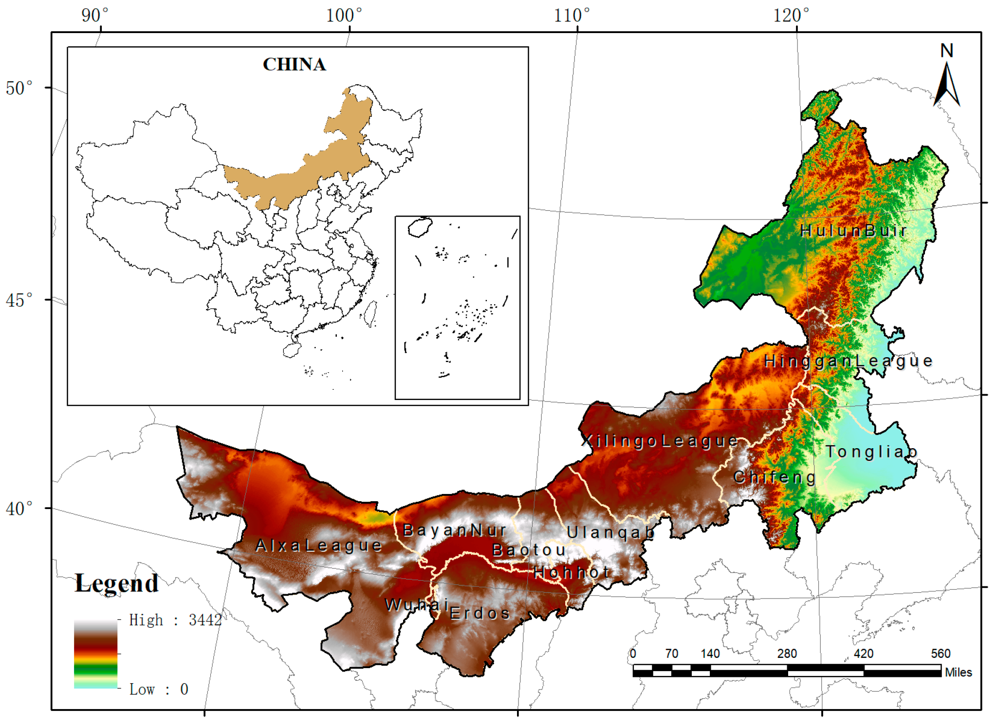
2.1. Study Area
2.2. Data Sources
2.3. Methods
2.3.1. Spatial Autocorrelation Theory
2.3.2. Cold and Hot Spot Analysis
2.3.3. Spatial Regression Analysis of Influencing Factors
- Stepwise Multiple Regression
- Introduce variables one by one to construct a linear regression model of the dependent variable with i independent variables:
- 2.
- For each variable added to the model, use hypothesis testing to determine whether it significantly improves the model fit. Generally, t-statistics or F-statistics are used to test the significance of coefficients. If the result is significant, the variable is retained in the model; otherwise, it is removed.
- 3.
- Repeat the above steps to gradually introduce or eliminate variables until no further variables can be added or removed, ultimately obtaining the optimal model, which is as follows:
- Geographically Weighted Regression (GWR)
3. Results
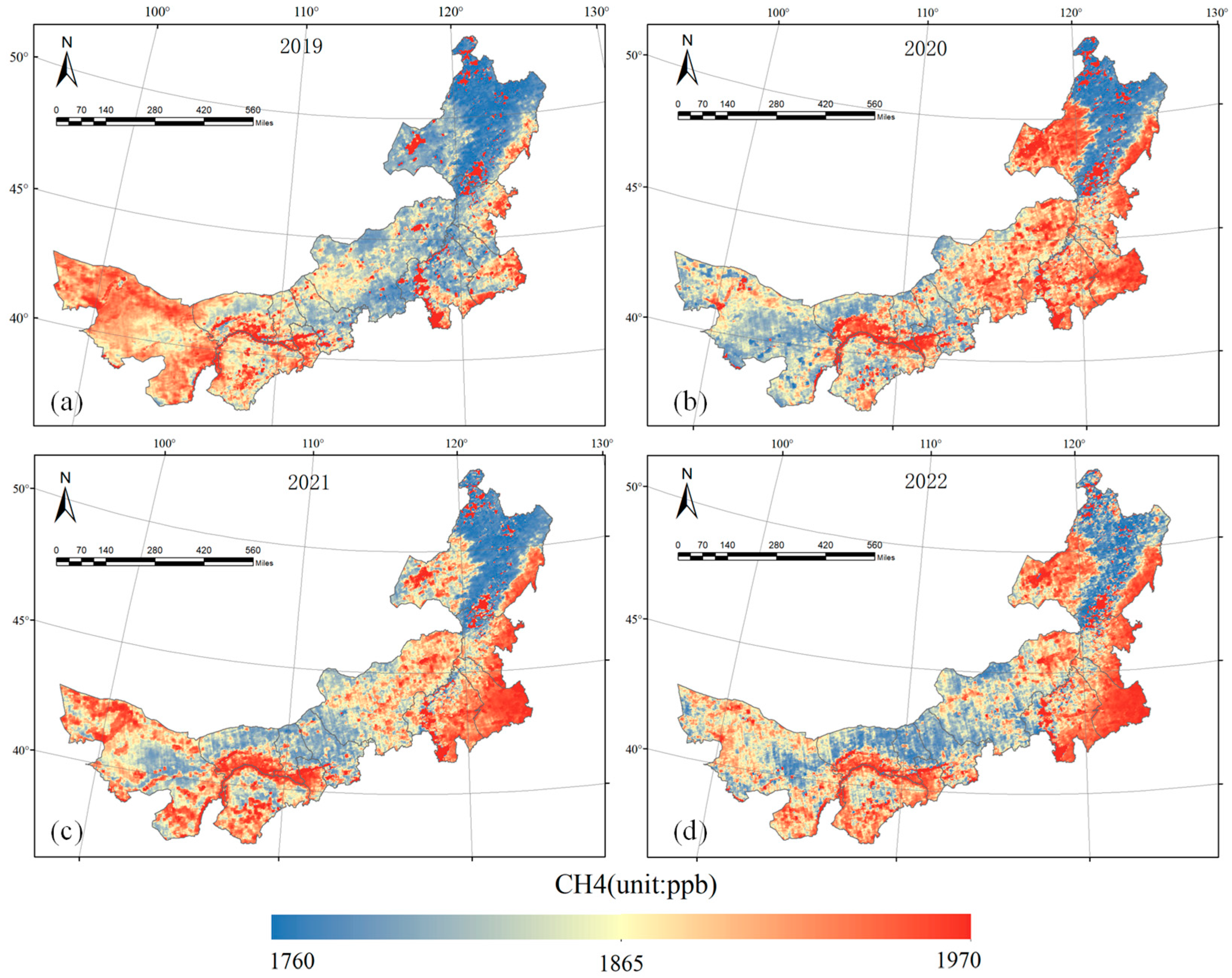
3.1. Spatial Distribution of CH4
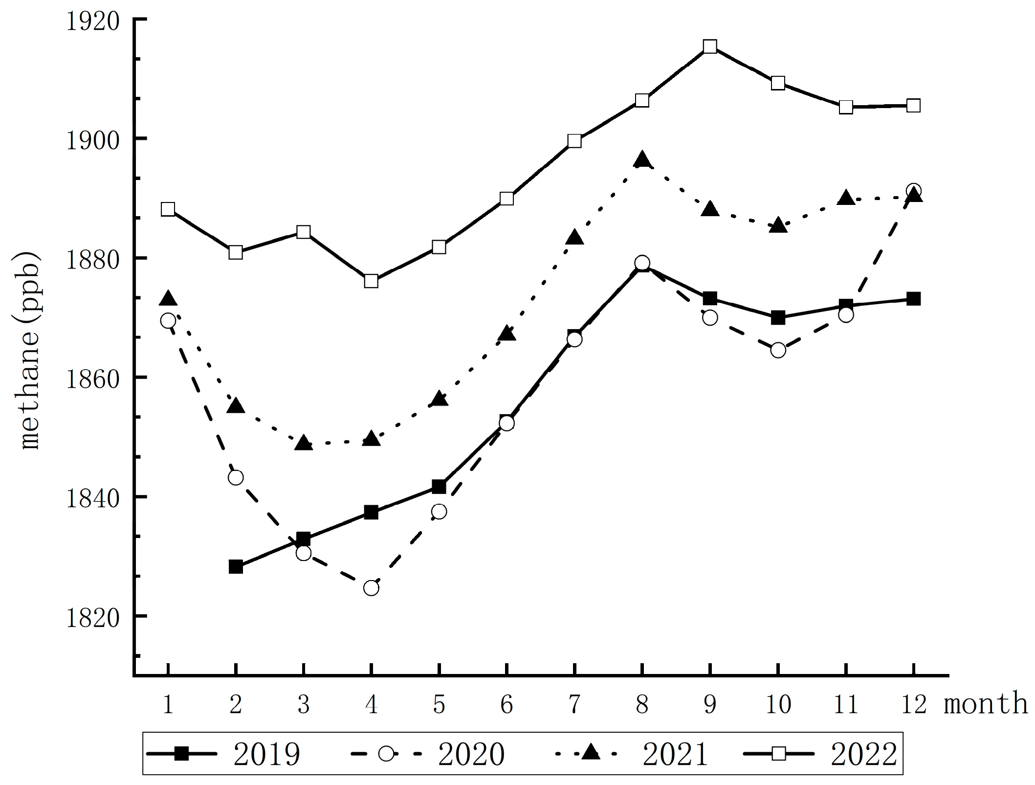
3.1.1. Temporal Distribution of CH4
3.1.2. Driving Factor Analysis of CH4
- Stepwise Multiple Regression Analysis
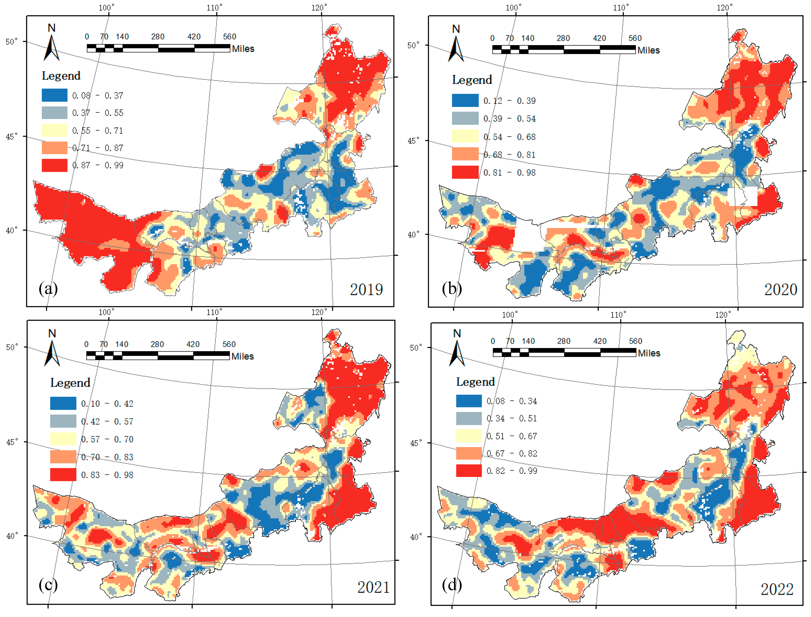
- Geographically Weighted Regression (GWR)
4. Conclusions
- From 2019 to 2022, the methane concentration in Inner Mongolia exhibited significant spatial clustering characteristics, with high-value areas primarily concentrated in the southeast and low-value areas in the central region. Overall, the methane concentration in Inner Mongolia showed an increasing trend year by year, maintaining a relatively stable spatial distribution pattern characterized by lower concentrations in the east and north and higher concentrations in the west and south. Temporally, the methane levels in Inner Mongolia displayed clear seasonal fluctuations, being higher in summer and lower in spring, with a cyclical pattern of change. Typically, the concentrations decreased in March to April and rose rapidly from June to August. Notably, Tongliao City, with its developed agriculture and animal husbandry, and Wuhai City and Alxa League, with sparse vegetation and rich coal resources, exhibited relatively high methane concentrations, while Baotou and Hulunbuir had relatively low concentrations.
- The effects of the five drivers on the methane concentration in Inner Mongolia were differentiated. The multiple stepwise regression analysis showed that precipitation (PRE) and soil temperature (SOIL_TEMP) had continuous positive effects, while human activity intensity (DNB) had a weak effect, and vegetation index (NDVI) and surface temperature (LST) had inhibitory effects. There is a reciprocal relationship between methane emissions and climate change. Precipitation, temperature, and the vegetation index influence methane emissions by regulating soil moisture and the living environment of methanogens. Additionally, human activities, particularly grazing, significantly affected the methane absorption and emission processes. Notably, the impact of different drivers on the methane concentrations exhibited distinct spatial heterogeneity. After considering the spatial location factors, the overall goodness of fit of the geographically weighted regression model was significantly improved compared to the multiple stepwise regression model, especially in areas with higher methane concentrations.
Author Contributions
Funding
Institutional Review Board Statement
Informed Consent Statement
Data Availability Statement
Acknowledgments
Conflicts of Interest
References
- Cao, Y.; Li, X.M.; Yan, H.B.; Kuang, S.Y. China’s efforts to peak carbon emissions: Targets and practice. Chin. J. Urban Environ. Stud. 2021, 9, 2150004. [Google Scholar] [CrossRef]
- Shindell, D.; Kuylenstierna, J.C.; Vignati, E.; van Dingenen, R.; Amann, M.; Klimont, Z.; Anenberg, S.C.; Muller, N.; Janssens-Maenhout, G.; Raes, F.; et al. Simultaneously mitigating near-term climate change and improving human health and food security. Science 2012, 335, 183–189. [Google Scholar] [CrossRef] [PubMed]
- Saunois, M.; Jackson, R.B.; Bousquet, P.; Poulter, B.; Canadell, J.G. The growing role of methane in anthropogenic climate change. Environ. Res. Lett. 2016, 11, 120207. [Google Scholar] [CrossRef]
- Lan, X.; Thoning, K.W.; Dlugokencky, E.J. Trends in Globally Averaged CH4, N2O, and SF6 Determined from NOAA Global Monitoring Laboratory Measurements; Version 2022-10; Global Monitoring Laboratory: Niwot Ridge, CO, USA, 2022. [Google Scholar] [CrossRef]
- Derwent, R.G. Global warming potential (GWP) for methane: Monte Carlo analysis of the uncertainties in global tropospheric model predictions. Atmosphere 2020, 11, 486. [Google Scholar] [CrossRef]
- Ocko, I.B.; Sun, T.; Shindell, D.; Oppenheimer, M.; Hristov, A.N.; Pacala, S.W.; Mauzerall, D.L.; Xu, Y.; Hamburg, S.P. Acting rapidly to deploy readily available methane mitigation measures by sector can immediately slow global warming. Environ. Res. Lett. 2021, 16, 054042. [Google Scholar] [CrossRef]
- Skytt, T.; Nielsen, S.N.; Jonsson, B.-G. Global warming potential and absolute global temperature change potential from carbon dioxide and methane fluxes as indicators of regional sustainability—A case study of Jämtland, Sweden. Ecol. Indic. 2020, 110, 105831. [Google Scholar] [CrossRef]
- Gore, A. Measure emissions to manage emissions. Science 2022, 378, 455. [Google Scholar] [CrossRef]
- Rehman, A.; Ma, H.; Irfan, M.; Ahmad, M. Does carbon dioxide, methane, nitrous oxide, and GHG emissions influence the agriculture? Evidence from China. Environ. Sci. Pollut. Res. 2020, 27, 28768–28779. [Google Scholar] [CrossRef]
- Schwietzke, S.; Sherwood, O.A.; Bruhwiler, L.M.; Miller, J.B.; Etiope, G.; Dlugokencky, E.J.; Michel, S.E.; Arling, V.A.; Vaughn, B.H.; White, J.W.; et al. Upward revision of global fossil fuel methane emissions based on isotope database. Nature 2016, 538, 88–91. [Google Scholar] [CrossRef]
- Devi, T.N.; Devi, A.S.; Singh, K.R. Emission of Methane from Wetland Paddy Fields: A Review. J. Clim. Chang. 2022, 8, 13–19. [Google Scholar] [CrossRef]
- Kuhla, B.; Viereck, G. Enteric methane emission factors, total emissions and intensities from Germany’s livestock in the late 19th century: A comparison with the today’s emission rates and intensities. Sci. Total Environ. 2022, 848, 157754. [Google Scholar] [CrossRef] [PubMed]
- Wang, G.; Liu, P.; Hu, J.; Zhang, F. Spatiotemporal Patterns and Influencing Factors of Agriculture Methane Emissions in China. Agriculture 2022, 12, 1573. [Google Scholar] [CrossRef]
- Luke. Comparing satellite methane measurements to inventory estimates: A Canadian case study. Atmos. Environ. X 2023, 17, 100198. [Google Scholar]
- De Gouw, J.A.; Veefkind, J.P.; Roosenbrand, E.; Dix, B.; Lin, J.C.; Landgraf, J.; Levelt, P.F. Daily Satellite observations of Methane from oil and Gas production Regions in the United States. Sci. Rep. 2020, 10, 1379. [Google Scholar] [CrossRef] [PubMed]
- IEA. Global Methane Tracker 2022. IEA, 2022, Paris. Licence: CC BY 4.0. Available online: https://www.iea.org/reports/global-methane-tracker-2022 (accessed on 1 February 2023).
- Wei, Y.; Yang, X.; Qiu, X.; Wei, H.; Tang, C. Spatio-temporal variations of atmospheric methane and its response to climate on the Tibetan Plateau from 2010 to 2022. Atmos. Environ. 2023, 314, 120088. [Google Scholar] [CrossRef]
- Zhang, Y.; Fang, S.; Chen, J.; Lin, Y.; Chen, Y.; Liang, R.; Jiang, K.; Parker, R.J.; Boesch, H.; Steinbacher, M.; et al. Observed changes in China’s methane emissions linked to policy drivers. Proc. Natl. Acad. Sci. USA 2022, 41, e2202742119. [Google Scholar] [CrossRef] [PubMed]
- He, B.; Xue, Y.; Ling, X.; Lu, X.; Liu, W.; Wang, X. Temporal and Spatial Distribution of Atmospheric CH4 Concentration and Estimation of Animal Husbandry Emissions in Hebei Province. In Proceedings of the IGARSS 2022—2022 IEEE International Geoscience and Remote Sensing Symposium, Kuala Lumpur, Malaysia, 17–22 July 2022. [Google Scholar]
- Martin, R.V. Satellite remote sensing of air quality. Atmos. Environ. 2008, 42, 7823–7843. [Google Scholar] [CrossRef]
- Schneising, O.; Burrows, J.P.; Dickerson, R.R.; Buchwitz, M.; Reuter, M.; Bovensmann, H. Remote sensing of fugitive methane emissions from oil and gas production in North American tight geologic formations. Earth’s Future 2014, 2, 548–558. [Google Scholar] [CrossRef]
- Kort, E.A.; Frankenberg, C.; Costigan, K.R.; Lindenmaier, R.; Dubey, M.K.; Wunch, D. Four corners: The largest US methane anomaly viewed from space. Geophys. Res. Lett. 2014, 41, 6898–6903. [Google Scholar] [CrossRef]
- Veefkind, J.; Aben, I.; McMullan, K.; Förster, H.; de Vries, J.; Otter, G.; Claas, J.; Eskes, H.; de Haan, J.; Kleipool, Q. TROPOMI on the ESA Sentinel-5 Precursor: A GMES mission for global observations of the atmospheric composition for climate, air quality and ozone layer applications. Remote Sens. Environ. 2012, 120, 70–83. [Google Scholar] [CrossRef]
- Schneising, O.; Buchwitz, M.; Reuter, M.; Vanselow, S.; Bovensmann, H.; Burrows, J.P. Remote sensing of methane leakage from natural gas and petroleum systems revisited. Atmos. Chem. Phys. 2020, 20, 9169–9182. [Google Scholar] [CrossRef]
- Lorente, A.; Borsdorff, T.; Butz, A.; Hasekamp, O.; de Brugh, J.A.; Schneider, A.; Hase, F.; Kivi, R.; Wunch, D.; Pollard, D.F.; et al. Methane retrieved from TROPOMI: Improvement of the data product and validation of the first two years of measurements. Atmos. Meas. Tech. 2021, 14, 665–684. [Google Scholar] [CrossRef]
- ESA. Algorithm Theoretical Baseline Document for Sentinel-5P Methane Retrieval. European Space Agency. 2021. Available online: https://sentinel.esa.int/documents/247904/2476257/Sentinel-5P-TROPOMI-ATBD-Methane-retrieval.pdf/f275eb1d-89a8-464f-b5b8-c7156cda874e?version=1.1 (accessed on 10 February 2023).
- Yang, Y.; Zhou, M.; Langerock, B.; Sha, M.K.; Hermans, C.; Wang, T.; Ji, D.; Vigouroux, C.; Kumps, N.; Wang, G.; et al. New ground-based Fourier-transform near-infrared solar absorption measurements of XCO2, XCH4 and XCO at Xianghe, China. Earth Syst. Sci. Data 2020, 12, 1679–1696. [Google Scholar] [CrossRef]
- Schneising, O.; Buchwitz, M.; Reuter, M.; Bovensmann, H.; Burrows, J.P.; Borsdorff, T.; Deutscher, N.M.; Feist, D.G.; Griffith, D.W.T.; Hase, F.; et al. A scientific algorithm to simultaneously retrieve carbon monoxide and methane from TROPOMI onboard Sentinel-5 Precursor. Atmos. Meas. Tech. 2019, 12, 6771–6802. [Google Scholar] [CrossRef]
- Cui, H.; Wang, Y.; Su, X.; Wei, S.; Pang, S.; Zhu, Y.; Zhang, S.; Ma, C.; Hou, W.; Jiang, H. Response of methanogenic community and their activity to temperature rise in alpine swamp meadow at different water level of the permafrost wetland on Qinghai-Tibet Plateau. Front. Microbiol. 2023, 14, 1181658. [Google Scholar] [CrossRef] [PubMed]
- Chen, H.; Ju, P.; Zhu, Q.; Xu, X.; Wu, N.; Gao, Y.; Feng, X.; Tian, J.; Niu, S.; Zhang, Y. Carbon and nitrogen cycling on the Qinghai–Tibetan plateau. Nat. Rev. Earth Environ. 2022, 3, 701–716. [Google Scholar] [CrossRef]
- Zhang, X.M.; Zhang, X.Y.; Zhu, Q.A.; Jiang, H.; Li, X.H.; Cheng, M. Spatial distribution simulation and the climate effects of aerobic methane emissions from terrestrial plants in China. Acta Ecol. Sin. 2016, 36, 580–591. [Google Scholar]
- Tang, S.; Zhang, Y.; Zhai, X.; Wilkes, A.; Wang, C.; Wang, K. Effect of grazing on methane uptake from Eurasian steppe of China. BMC Ecol. 2018, 18, 16. [Google Scholar] [CrossRef]


| Impact Factor | Product | Band Name | Spatial Resolution | Temporal Resolution |
|---|---|---|---|---|
| Human activity intensity | VIIRS Stray Light Corrected Nighttime Day/Night Band Composites | avg_rad | 500m | monthly |
| Vegetation coverage | MOD13A2.006 Terra Vegetation Indices 16-Day Global 1 km | NDVI | 1km | 16 day |
| Soil Temperature | ERA5-Land Daily Aggregated—ECMWF Climate Reanalysis | soil_temperature level_1 | 0.1° | daily |
| Precipitation | GPM: Global Precipitation Measurement | precipitaioncal | 0.1° | daily |
| Land Surface Temperature | MOD11A2.006 Terra Land Surface Temperature and Emissivity 8-Day | LST_Day_1km | 1km | 8 day |
| Indicator | Definition |
|---|---|
| Day/Night Band (DNB) | representing nocturnal light intensity as a proxy for human activity |
| Normalized Difference Vegetation Index (NDVI) | used for assessing vegetation coverage and growth status |
| Soil Temperature (SOIL_TEMP) | indicating the temperature of the soil |
| Precipitation (PRE) | representing the amount of rainfall |
| Land Surface Temperature (LST) | indicating the temperature of Earth’s surface |
| Impact Factor | 2019 | 2020 | 2021 | 2022 |
|---|---|---|---|---|
| PRE | 0.168 * | 0.470 * | 0.320 * | 0.280 * |
| NDVI | −0.315 * | −0.546 * | −0.398 * | −0.206 * |
| LST | - | −0.308 * | −0.184 * | −0.120 * |
| SOIL_TEMP | 0.231 * | 0.372 * | 0.345 * | 0.189 * |
| DNB | - | 0.184 * | 0.124 * | 0.139 * |
| R2 | 0.579 | 0.496 * | 0.494 * | 0.505 * |
Disclaimer/Publisher’s Note: The statements, opinions and data contained in all publications are solely those of the individual author(s) and contributor(s) and not of MDPI and/or the editor(s). MDPI and/or the editor(s) disclaim responsibility for any injury to people or property resulting from any ideas, methods, instructions or products referred to in the content. |
© 2024 by the authors. Licensee MDPI, Basel, Switzerland. This article is an open access article distributed under the terms and conditions of the Creative Commons Attribution (CC BY) license (https://creativecommons.org/licenses/by/4.0/).
Share and Cite
Yan, S.; Xie, Y.; Han, G.; Meng, X.; Li, Z. Methane Dynamics in Inner Mongolia: Unveiling Spatial and Temporal Variations and Driving Factors. Proceedings 2024, 110, 29. https://doi.org/10.3390/proceedings2024110029
Yan S, Xie Y, Han G, Meng X, Li Z. Methane Dynamics in Inner Mongolia: Unveiling Spatial and Temporal Variations and Driving Factors. Proceedings. 2024; 110(1):29. https://doi.org/10.3390/proceedings2024110029
Chicago/Turabian StyleYan, Sirui, Yichun Xie, Ge Han, Xiaoliang Meng, and Ziwei Li. 2024. "Methane Dynamics in Inner Mongolia: Unveiling Spatial and Temporal Variations and Driving Factors" Proceedings 110, no. 1: 29. https://doi.org/10.3390/proceedings2024110029
APA StyleYan, S., Xie, Y., Han, G., Meng, X., & Li, Z. (2024). Methane Dynamics in Inner Mongolia: Unveiling Spatial and Temporal Variations and Driving Factors. Proceedings, 110(1), 29. https://doi.org/10.3390/proceedings2024110029