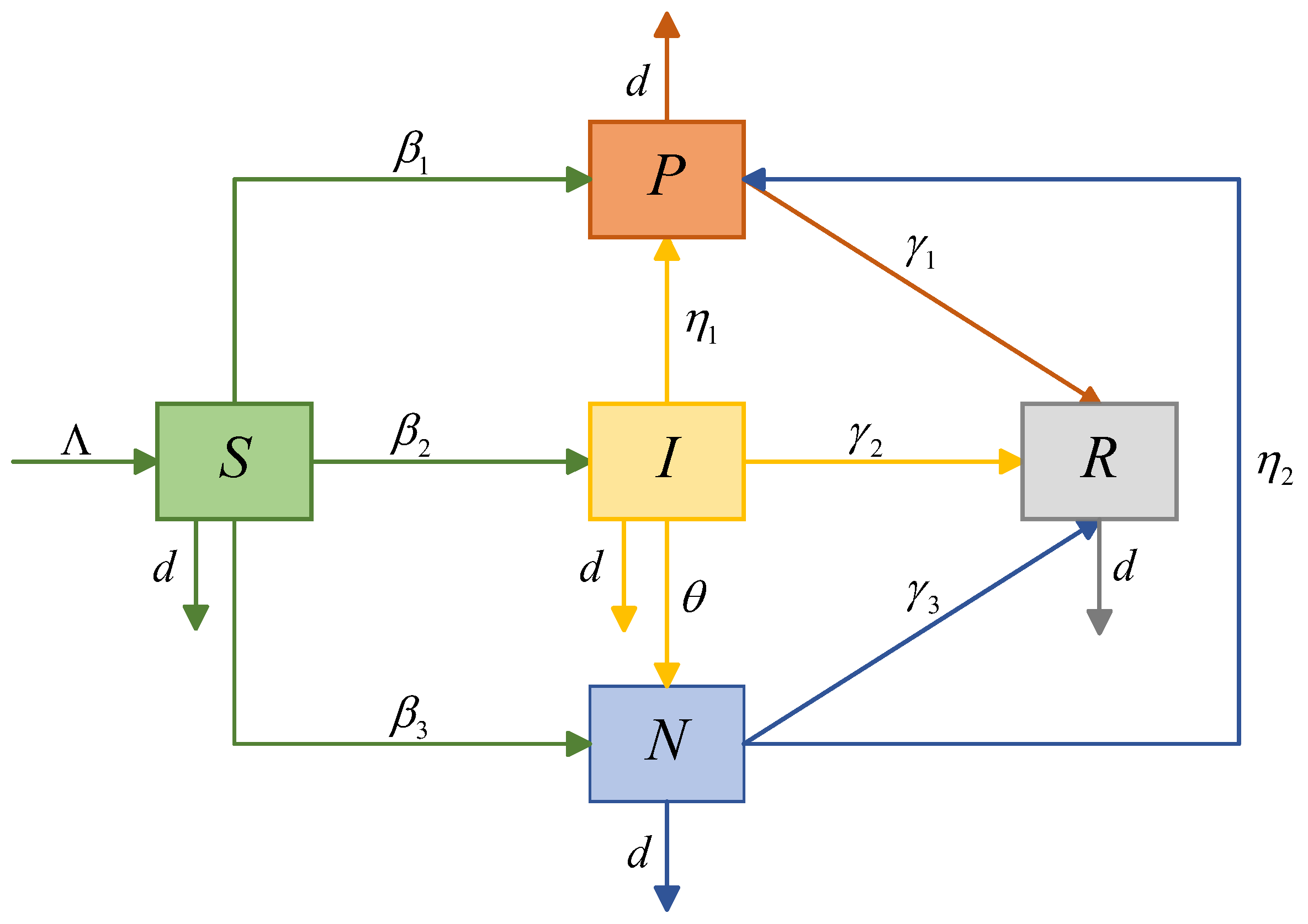
Figure 1.
The state transition diagram of the SINPR model.
Figure 1.
The state transition diagram of the SINPR model.
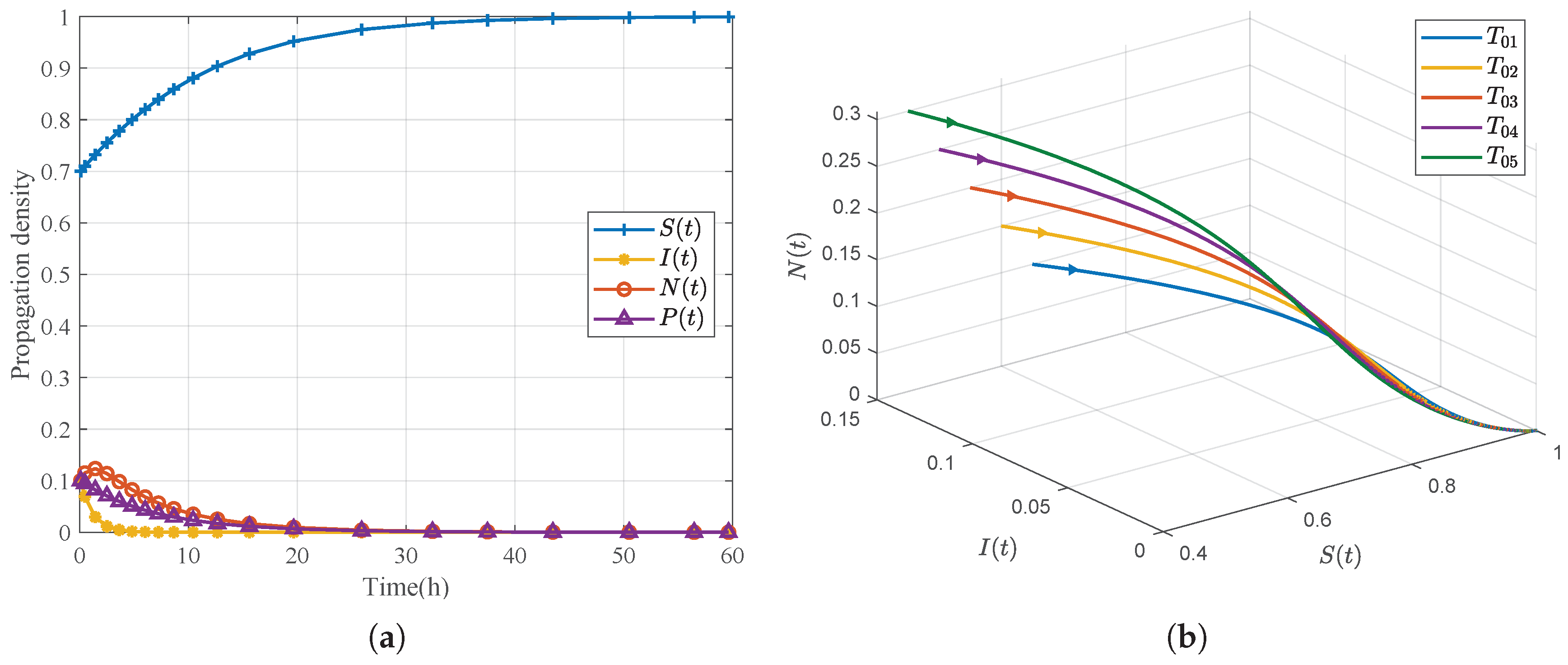
Figure 2.
Rumor-free equilibrium : (a) time evolution of the densities , , , and ; (b) phase diagram for five distinct initial values.
Figure 2.
Rumor-free equilibrium : (a) time evolution of the densities , , , and ; (b) phase diagram for five distinct initial values.
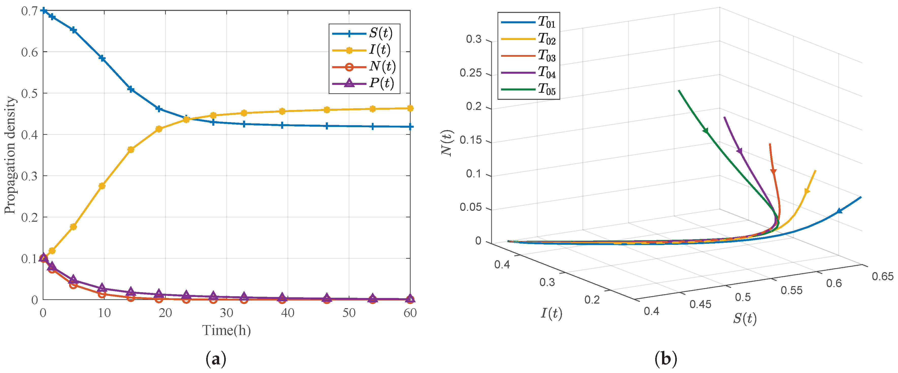
Figure 3.
Boundary equilibrium : (a) time evolution of the densities , , , and ; (b) phase diagram for five distinct initial values.
Figure 3.
Boundary equilibrium : (a) time evolution of the densities , , , and ; (b) phase diagram for five distinct initial values.
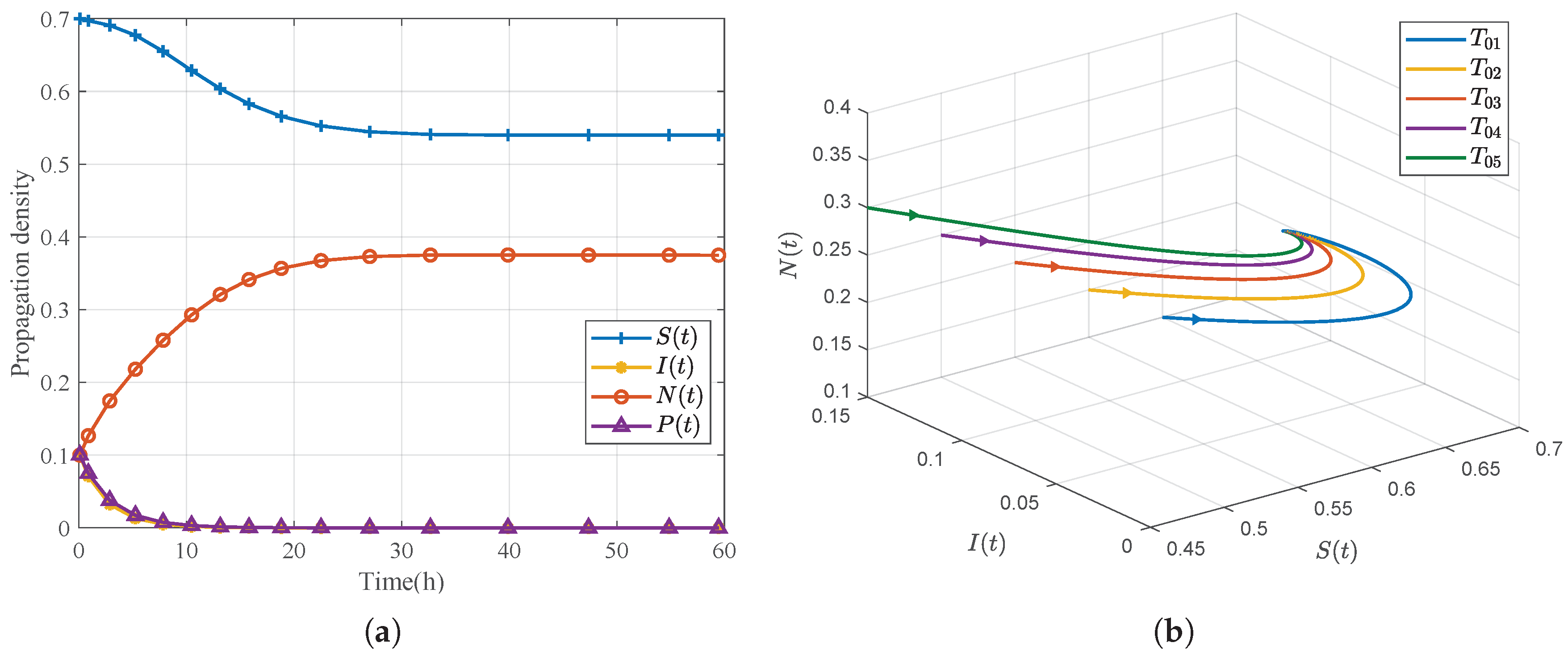
Figure 4.
Boundary equilibrium : (a) time evolution of the densities , , , and ; (b) phase diagram for five distinct initial values.
Figure 4.
Boundary equilibrium : (a) time evolution of the densities , , , and ; (b) phase diagram for five distinct initial values.
Figure 5.
Boundary equilibrium : (a) time evolution of the densities , , , and ; (b) phase diagram for five distinct initial values.
Figure 5.
Boundary equilibrium : (a) time evolution of the densities , , , and ; (b) phase diagram for five distinct initial values.
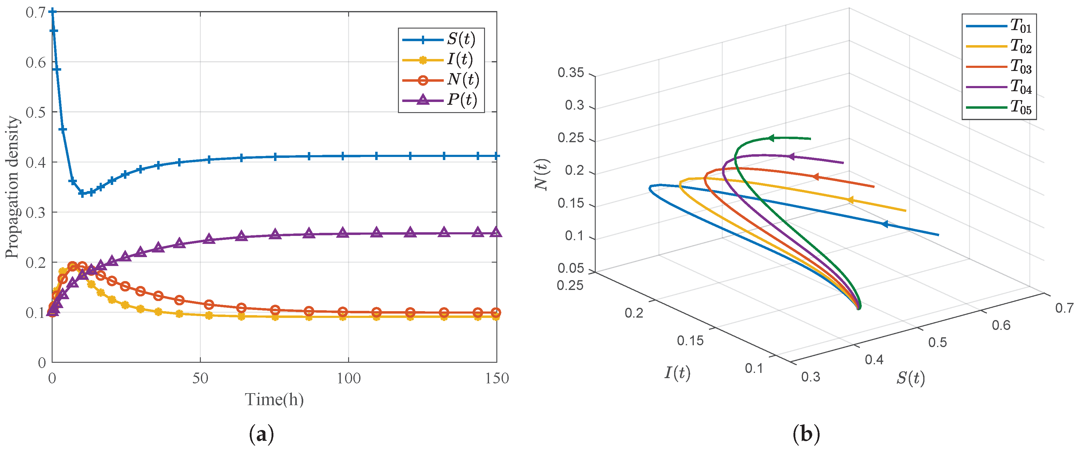
Figure 6.
Coexistence equilibrium : (a) time evolution of the densities , , , and ; (b) phase diagram for five distinct initial values.
Figure 6.
Coexistence equilibrium : (a) time evolution of the densities , , , and ; (b) phase diagram for five distinct initial values.
Figure 7.
Sensitivity indices with respect to different parameters: (a) , (b) , and (c) .
Figure 7.
Sensitivity indices with respect to different parameters: (a) , (b) , and (c) .
Figure 8.
Threshold : (a) relationship between and , (b) relationship between d and , and (c) combined effect of and d on .
Figure 8.
Threshold : (a) relationship between and , (b) relationship between d and , and (c) combined effect of and d on .
Figure 9.
Threshold : (a) relationship between d and , (b) relationship between and , and (c) combined effect of d and on .
Figure 9.
Threshold : (a) relationship between d and , (b) relationship between and , and (c) combined effect of d and on .
Figure 10.
Threshold : (a) relationship between and , (b) relationship between and , and (c) combined effect of and on .
Figure 10.
Threshold : (a) relationship between and , (b) relationship between and , and (c) combined effect of and on .
Figure 11.
Transcritical bifurcation at (a) , (b) , and (c) .
Figure 11.
Transcritical bifurcation at (a) , (b) , and (c) .
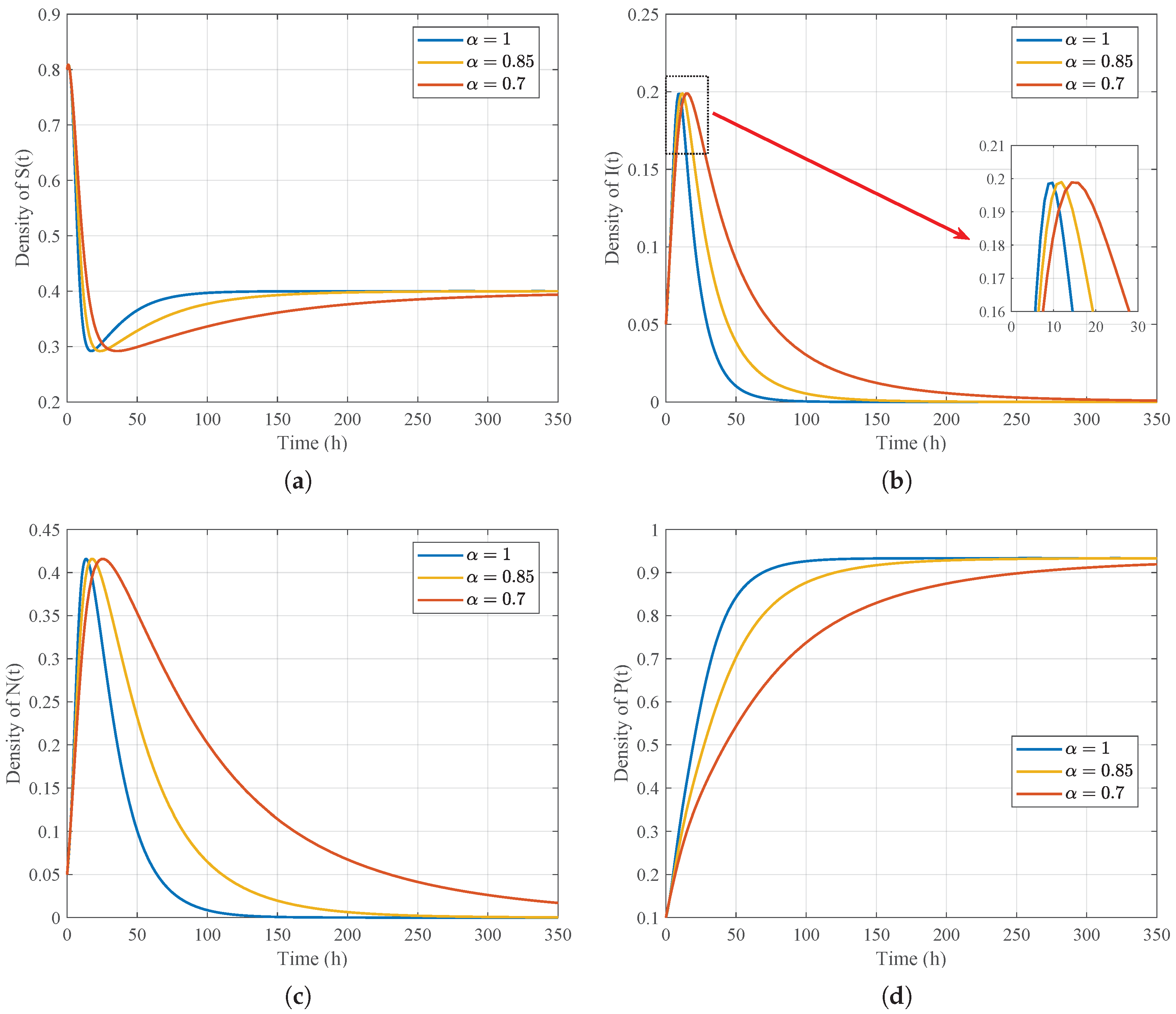
Figure 12.
Density evolution of state variables under different fractional orders : (a) , (b) , (c) , and (d) .
Figure 12.
Density evolution of state variables under different fractional orders : (a) , (b) , (c) , and (d) .
Figure 13.
Density evolution of under different initial conditions: (a) , (b) , (c) , and (d) .
Figure 13.
Density evolution of under different initial conditions: (a) , (b) , (c) , and (d) .
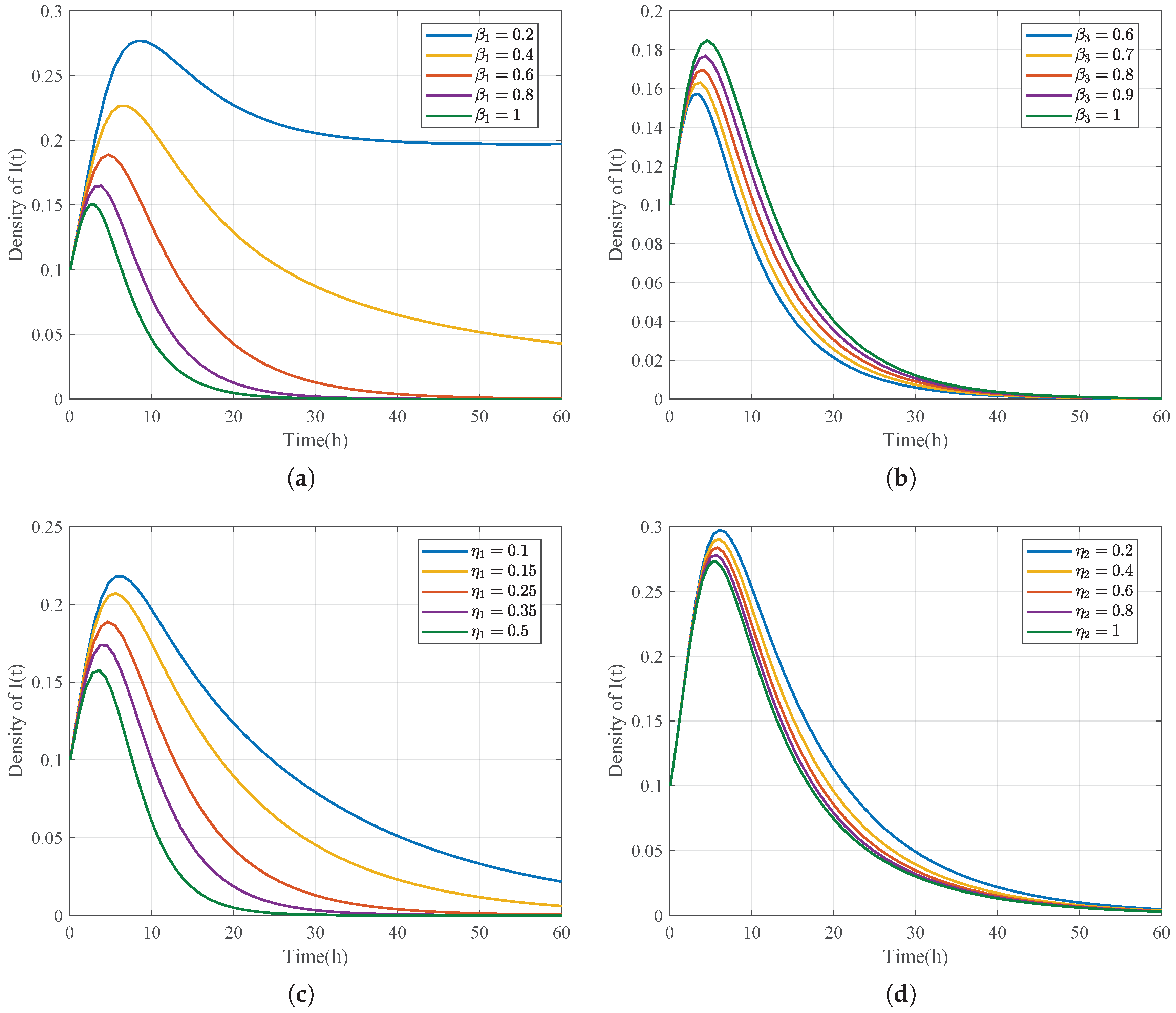
Figure 14.
Impact of emotional mechanisms on the density of rumor spreaders with varying parameters: (a) , (b) , (c) , and (d) .
Figure 14.
Impact of emotional mechanisms on the density of rumor spreaders with varying parameters: (a) , (b) , (c) , and (d) .
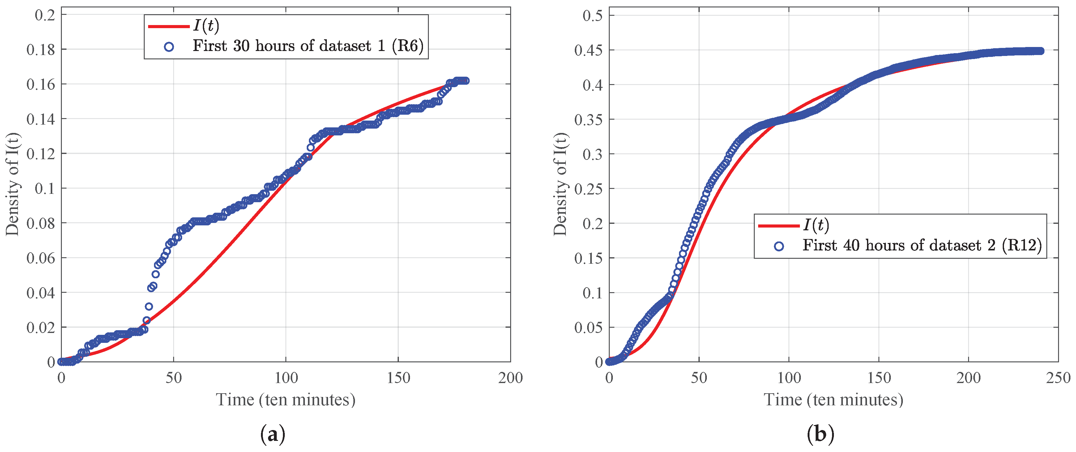
Figure 15.
The fitting curve for the I state and the actual data for the rumor datasets: (a) dataset 1 (R6); (b) dataset 2 (R12).
Figure 15.
The fitting curve for the I state and the actual data for the rumor datasets: (a) dataset 1 (R6); (b) dataset 2 (R12).
Figure 16.
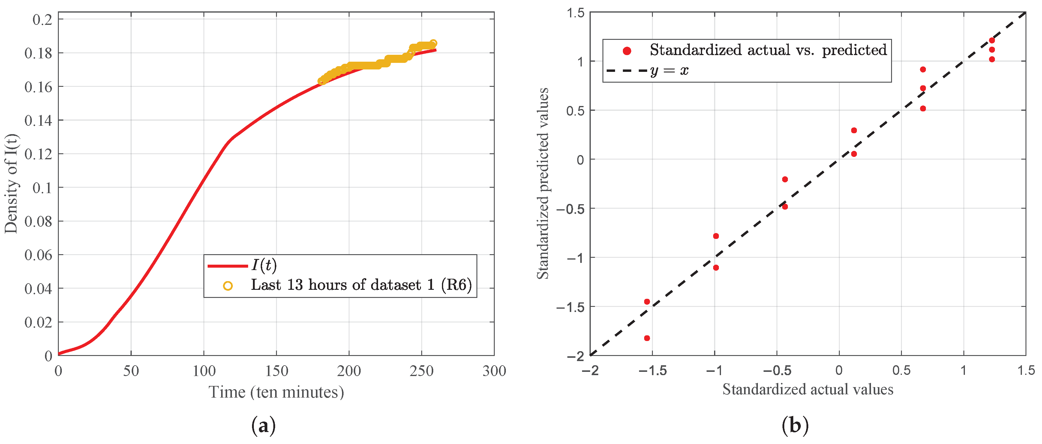
Dataset 1 (R6): (a) prediction curve for the I state and actual data in the last 13 h; (b) standardized predicted values vs. standardized actual values.
Figure 16.
Dataset 1 (R6): (a) prediction curve for the I state and actual data in the last 13 h; (b) standardized predicted values vs. standardized actual values.
Figure 17.
Dataset 2 (R12): (a) prediction curve for the I state and actual data in the last 36 h; (b) standardized predicted values vs. standardized actual values.
Figure 17.
Dataset 2 (R12): (a) prediction curve for the I state and actual data in the last 36 h; (b) standardized predicted values vs. standardized actual values.
Figure 18.
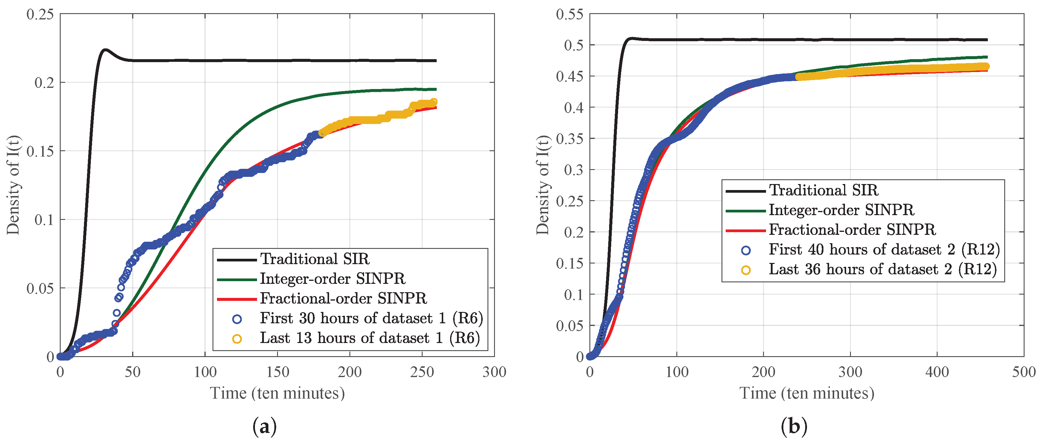
Comparison of the density evolution of for the traditional SIR model, integer-order SINPR model, and fractional-order SINPR model with different datasets: (a) dataset 1 (R6); (b) dataset 2 (R12).
Figure 18.
Comparison of the density evolution of for the traditional SIR model, integer-order SINPR model, and fractional-order SINPR model with different datasets: (a) dataset 1 (R6); (b) dataset 2 (R12).
Table 1.
Description of parameters in the SINPR model.
Table 1.
Description of parameters in the SINPR model.
| Category | Symbol | Parameter Description |
|---|
| Inflow rate | | Population inflow rate into the social network per unit time |
| Outflow rate | d | Population outflow rate from the social network per unit time |
| Infection rate | | Probability susceptibles are infected by positive emotion spreaders |
| Probability susceptibles are infected by rumor spreaders |
| Probability susceptibles are infected by negative emotion spreaders |
| Purification rate | | Conversion rate of rumor spreaders due to positive emotion purification |
| Conversion rate of negative emotion spreaders due to positive emotion purification |
| Instigation rate | | Rate at which rumor spreaders are driven by negative emotion instigation |
| Immunity rate | | Rate at which positive emotion spreaders become immune |
| Rate at which rumor spreaders become immune |
| Rate at which negative emotion spreaders become immune |
Table 2.
Parameters for the local stability of , , , , and .
Table 2.
Parameters for the local stability of , , , , and .
| Parameter | | d | | | | | | | | | |
|---|
| Data 1 () | 0.15 | 0.15 | 0.1 | 0.1 | 0.1 | 0.7 | 0.2 | 0.2 | 0.1 | 0.1 | 0.1 |
| Data 2 () | 0.19 | 0.19 | 0.48 | 0.3 | 0.25 | 0.3 | 0.3 | 0.2 | 0.05 | 0.11 | 0.11 |
| Data 3 () | 0.2 | 0.2 | 0.25 | 0.6 | 0.2 | 0 | 0.5 | 0.05 | 0.2 | 0.05 | 0.15 |
| Data 4 () | 0.22 | 0.22 | 0.25 | 0.25 | 0.5 | 0.3 | 0.25 | 0.2 | 0.35 | 0.05 | 0.05 |
| Data 5 () | 0.16 | 0.16 | 0.37 | 0.86 | 0.55 | 0.08 | 0.25 | 0.35 | 0.05 | 0.05 | 0.05 |
Table 3.
Parameters for the sensitivity of , , and .
Table 3.
Parameters for the sensitivity of , , and .
| Parameter | | d | | | | | | | | | |
|---|
| Data 1 () | 0.2 | 0.2 | 0.2 | 0.5 | 0.2 | 0.1 | 0.1 | 0.1 | 0.15 | 0.1 | 0.15 |
| Data 2 () | 0.2 | 0.2 | 0.3 | 0.4 | 0.35 | 0.2 | 0.1 | 0.1 | 0.10 | 0.15 | 0.05 |
| Data 3 () | 0.2 | 0.2 | 0.4 | 0.2 | 0.15 | 0.2 | 0.1 | 0.1 | 0.1 | 0.15 | 0.15 |
Table 4.
Parameters for the transcritical bifurcation of , , and .
Table 4.
Parameters for the transcritical bifurcation of , , and .
| Parameter | | d | | | | | | | | | |
|---|
| Data 1 () | 0.2 | 0.2 | 0.2 | [0.001–1] | 0.2 | 0.1 | 0.1 | 0.15 | 0.15 | 0.1 | 0.15 |
| Data 2 () | 0.2 | 0.2 | 0.2 | 0.3 | [0.001–1] | 0.3 | 0.2 | 0.25 | 0.15 | 0.2 | 0.2 |
| Data 3 () | 0.2 | 0.2 | [0.001–1] | 0.4 | 0.4 | 0.25 | 0.3 | 0.25 | 0.1 | 0.15 | 0.2 |
Table 5.
Parameters influencing dynamic evolution of rumor propagation.
Table 5.
Parameters influencing dynamic evolution of rumor propagation.
| Parameter | | d | | | | | | | | | |
|---|
| Data 1 | 0.14 | 0.07 | 0.3 | 0.55 | 0.5 | 0.04 | 0.10 | 0.15 | 0.05 | 0.08 | 0.04 |
| Data 2 | 0.16 | 0.06 | 0.28 | 0.50 | 0.55 | 0.05 | 0.12 | 0.14 | 0.045 | 0.07 | 0.06 |
| Data 3 | 0.15 | 0.13 | [0.2–1] | 0.8 | 0.55 | 0.05 | 0.25 | 0.35 | 0.05 | 0.05 | 0.05 |
| Data 4 | 0.15 | 0.13 | 0.6 | 0.8 | [0.6–1] | 0.05 | 0.25 | 0.35 | 0.05 | 0.05 | 0.05 |
| Data 5 | 0.15 | 0.13 | 0.6 | 0.8 | 0.55 | 0.05 | [0.1–0.5] | 0.35 | 0.05 | 0.05 | 0.05 |
| Data 6 | 0.15 | 0.13 | 0.6 | 0.9 | 0.05 | 0.05 | 0.25 | [0.2–1] | 0.05 | 0.03 | 0.01 |
Table 6.
Information of rumor datasets for experimental analysis.
Table 6.
Information of rumor datasets for experimental analysis.
| Dataset ID | Description | Total Tweets | Rumor Tweets | Collection Period |
|---|
| Dataset 1 (R6) | Harley-Davidson’s chief executive officer Matthew Levatich called President Trump “a moron”. | 754 | 140 | [‘2018’, ‘Jun’, ‘28’, ‘23:49:04’] [‘2018’, ‘Jun’, ‘30’, ‘17:55:51’] |
| Dataset 2 (R12) | A screenshot from MyLife.com confirms that mail bomb suspect Cesar Sayoc was registered as a Democrat. | 32,079 | 14,931 | [‘2018’, ‘Oct’, ‘26’, ‘16:01:36’] [‘2018’, ‘Oct’, ‘29’, ‘20:03:27’] |
Table 7.
Parameter values obtained by fitting.
Table 7.
Parameter values obtained by fitting.
| Parameter | | d | | | | | | | | | |
|---|
| Data 1 | 0.1782 | 0.2405 | 0.3794 | 0.8271 | 0.5875 | 0.0126 | 0.2484 | 0.3438 | 0.0685 | 0.0765 | 0.0256 |
| Data 2 | 0.2727 | 0.2067 | 0.3397 | 0.3483 | 0.2473 | 0.0001 | 0.2031 | 0.0016 | 0.1384 | 0.0418 | 0.0862 |
Table 8.
Model performance metrics for different datasets.
Table 8.
Model performance metrics for different datasets.
| Datasets | Model | Standardized | RMSE | MSE |
|---|
| Dataset 1 (R6) | Traditional SIR | 0.6683 | 0.0488 | 0.0024 |
| | Integer-order SINPR | 0.9202 | 0.0259 | 0.0007 |
| | Fractional-order SINPR | 0.9712 | 0.0090 | 0.0001 |
| Dataset 2 (R12) | Traditional SIR | 0.8358 | 0.0563 | 0.0032 |
| | Integer-order SINPR | 0.9427 | 0.0174 | 0.0003 |
| | Fractional-order SINPR | 0.9801 | 0.0006 | 0.0001 |
