Reliability Evaluation and Optimization of System with Fractional-Order Damping and Negative Stiffness Device

Abstract

Research on reliability control for enhancing power systems under random loads holds significant and undeniable importance in maintaining system stability, performance, and safety. The primary challenge lies in determining the reliability index while optimizing system parameters. To effectively address this challenge, we developed a novel intelligent algorithm and conducted an optimal reliability assessment for a Negative Stiffness Device (NSD) seismic isolation structure incorporating fractional-order damping. This algorithm combines the Gaussian Radial Basis Function Neural Network (GRBFNN) with the Particle Swarm Optimization (PSO) algorithm. It takes the reliability function with unknown parameters as the objective function, while using the Backward Kolmogorov (BK) equation, which governs the reliability function and is accompanied by boundary and initial conditions, as the constraint condition. During the operation of this algorithm, the neural network is employed to solve the BK equation, thereby deriving the fitness function in each iteration of the PSO algorithm. Then the PSO algorithm is utilized to obtain the optimal parameters. The unique advantage of this algorithm is its ability to simultaneously achieve the optimization of implicit objectives and the solution of time-dependent BK equations.To evaluate the performance of the proposed algorithm, this study compared it with the algorithm combines the GRBFNN with Genetic Algorithm (GA-GRBFNN)across multiple dimensions, including performance and operational efficiency. The effectiveness of the proposed algorithm has been validated through numerical comparisons and Monte Carlo simulations. The control strategy presented in this paper provides a solid theoretical foundation for improving the reliability performance of mechanical engineering systems and demonstrates significant potential for practical applications.

1. Introduction

Reliability, as a core indicator for evaluating the operational safety performance of power systems in complex vibration environments, plays a crucial role in ensuring the safety, functional stability, and durability of power systems, civil engineering structures, mechanical equipment, and aerospace infrastructure [1]. In recent years, with regard to extreme vibration scenarios such as earthquakes, research on reliability based on negative stiffness damping mechanisms has become a hot topic in the field of structural dynamics [2]. Under the condition of random load excitation, the core objective of reliability assessment for power systems is to quantify the probabilistic characteristics of system responses remaining within the safety domain, while reliability control aims to optimize and enhance reliability indicators by adjusting system parameters. Therefore, selecting appropriate control parameters is of great significance in achieving reliability objectives.

Within the analytical framework of stochastic dynamical systems, the probability density function is widely employed to characterize the statistical features of system uncertainties. Based on probabilistic distribution models, structural reliability assessment can be conducted using methods that include, but are not limited to, calculating the reliability function or failure probability of structures, or mean first-passage probability to analyze system failure mechanisms.

The concept of negative stiffness was first systematically proposed by Molyneaux in 1957 [3]. In his pioneering research, he designs a nonlinear vibration isolator that achieves the negative stiffness effect by constructing negative stiffness elements (NSE) using two symmetrically arranged inclined helical springs. Subsequently, Platus [4] further expanded the theoretical framework of negative stiffness mechanisms and developed a series of negative stiffness vibration isolation systems based on pre-compressed rods and preloaded flexible supports, covering vertical, horizontal, and six-degree-of-freedom vibration isolation systems. Carrella [5] and Mizuno [6] systematically demonstrated the remarkable effectiveness of this technology in vibration suppression through the experimental validation of negative stiffness vibration isolation systems. As research progressed, the principle of negative stiffness gradually permeated into the field of civil engineering. Ji [7] combined the negative stiffness mechanism with base isolation technology and proposes a novel composite isolation system that parallels a negative stiffness isolation layer with a traditional isolation system, conducting theoretical analysis and numerical simulation on its dynamic characteristics. Wu et al. [8] introduced negative stiffness magnetorheological dampers into the field of structural seismic response control, established a theoretical analysis model based on response spectra, and verified their seismic performance through real-time hybrid testing. Currently, various typical negative stiffness device schemes have been developed in research, including NSD-using Pre-loaded Elastic Elements [9], NSD-using Magnets [10], and Negative Stiffness Inter Damper [11]. Among these, the pre-compressed spring-type negative stiffness isolation system has demonstrated broad application prospects in engineering isolation due to its simple structure and reliable performance [12,13].

In recent years, the application of fractional derivative theory in the analysis of dynamical systems has garnered widespread attention. Compared with traditional integer-order models, the fractional derivative model has three advantages. Firstly, fractional derivatives can capture the memory effect and nonlocality of systems, effectively describing the correlation between the current state of a system and its historical inputs. This characteristic holds significant advantages in fields requiring the consideration of time-accumulation effects, such as the mechanics of viscoelastic materials [14]. Secondly, this theory provides a new mathematical tool for modeling the damping characteristics of complex systems, particularly in simulating the nonlinear viscous behavior of materials and non-continuous connection methods of structures, thereby breaking through the theoretical limitations of integer-order models [15]. Finally, the fractional derivative framework demonstrates stronger adaptability to nonlinear dynamical systems, enabling it to handle dynamic characteristics that traditional models cannot describe. It exhibits excellent robustness in engineering fields such as active vibration control and broadband noise suppression [16]. The characteristics make fractional derivative theory an important mathematical tool for analyzing the dynamic behaviors of complex dynamical systems, providing new theoretical support for the precise modeling and high-performance control of multi-physics coupled systems.

Reliability analysis, as a core approach for the safety assessment of engineering structures, has developed various mature theoretical frameworks. Mainstream analysis methods include the reliability index method [17], performance measurement approach [18], and sequential optimization and reliability assessment method [19]. In the field of earthquake engineering, due to the significant stochastic process characteristics of seismic excitation, reliability assessment methods based on first-passage have emerged as effective tools for quantifying the safety performance of control systems. By setting predefined safety threshold boundaries, this method can accurately characterize the dynamic reliability features of structures under random vibrations [20]. Recent research advancements have further deepened the application in this area: Taflanidis et al. [21] developed an efficient reliability design framework for tuned column damper systems, significantly enhancing control effectiveness under seismic action; Marano et al. [22] introduced constrained reliability theory into the optimization design of tuned mass dampers, achieving coordinated optimization of structural vibration control and reliability indicators; Mishra et al. [23] combined the first-passage model with base-isolated structures to establish a reliability-based structural optimization problem.

One of the most challenging core issues in reliability assessment under random loading conditions lies in solving the reliability control equations for nonlinear stochastic dynamical systems. To address this, it is necessary to construct system reliability models using probability theory and stochastic process theory [24], and derive the corresponding Backward Kolmogorov (BK) equations based on nonlinear stochastic dynamics and stochastic averaging principles. The BK equation is a parabolic time-varying partial differential equation (PDE) with specific initial and boundary conditions. Due to the existence of both first and second-order derivative terms in the equation, it is difficult to obtain exact analytical solutions. Currently, various numerical methods have been developed for solving the BK equation, including the finite difference method (FDM) [25,26], cell mapping method (CM) [27,28], and path integral method (PIM) [29,30], among others. However, these traditional methods all have inherent limitations. Therefore, there is a need to develop more efficient and robust numerical methods to achieve accurate solutions of the BK equation at arbitrary transient time steps, thereby breaking through the performance bottlenecks of existing technologies and providing more reliable theoretical support for the reliability analysis and control of nonlinear stochastic dynamical systems.

In recent years, with the breakthrough advancements in artificial intelligence technology, numerical methods based on three-layer Gaussian Radial Basis Function Neural Networks (GRBFNN) have demonstrated significant advantages in solving equations for complex stochastic dynamical systems. In 2023, Wang [31] applied GRBFNN to solve the Backward Kolmogorov (BK) equation in reliability control equations, exploring the probabilistic distribution characteristics of reliability functions for both linear and nonlinear dynamical systems, and validating the feasibility of this method in handling time-varying partial differential equations. In the same year, Li et al. [32] further expanded the application boundaries of GRBFNN by simultaneously obtaining both the time-varying reliability function and the mean first passage time for a class of stochastic dynamical systems’ BK equations. Chen [33] applied this method to study the dynamic behavior evolution of vibration-impact systems. By analyzing qualitative changes in probability distributions, he observed patterns of transient response variations and stochastic P-bifurcation phenomena. These works indicate that GRBFNN is an efficient algorithm with higher accuracy and efficiency, and even shorter runtime. It can be employed to investigate reliability control equations of systems under random loading conditions without introducing any controllers or optimization strategies to enhance reliability performance, focusing instead on theoretical exploration [34,35].

In reliability assessments under random loading conditions, another key challenge lies in maximizing reliability probability through specific reliability optimization methods under the BK equation and other constraints. The existing mainstream approaches primarily include the variational method [36] and the maximum principle [37,38]. The core advantage of the variational method is its ability to transform control problems into functional extremum problems, allowing for analytical solutions under ideal conditions. Meanwhile, the maximum principle converts optimal control problems into functional extremum conditions by constructing an augmented Hamiltonian system, providing the necessary conditions for stochastic optimal control. It is particularly noteworthy that traditional reliability optimization methods typically impose strict assumptions on the objective or value functions and heavily rely on solving the Euler–Lagrange equations or the Hamilton–Jacobi–Bellman (HJB) equations, facing significant computational challenges when dealing with high-dimensional or strongly nonlinear systems. Furthermore, the resulting control strategies often suffer from issues such as insufficient interpretability and limited engineering applicability. Therefore, there is a need to develop a novel optimization algorithm that minimizes theoretical complexity and numerical implementation difficulty while possessing the capability to perform stochastic reliability control for strongly nonlinear systems.

With advancements in machine learning and computer technology, the integration of traditional optimization algorithms with neural networks has demonstrated significant practicality in the field of reliability optimization. Cheng et al. [39,40] proposed an artificial neural network (ANN)-based genetic algorithm (GA) framework for reliability assessment of engineering structural systems: this method generates training datasets using the uniform design method, employs ANN to fit an explicit objective function, and combines it with an improved GA to achieve efficient estimation of failure probabilities. Gomes et al. [41] introduced a hybrid approach integrating GA with two types of neural networks (including a multilayer perceptron, MLP) for the reliability analysis of laminated composite structures, where the MLP is used to construct an explicit objective function for the GA, enabling the minimization of the total thickness of laminated composite plates through GA, with final reliability analysis performed using the First-Order Second-Moment (FOSM) method. Achraf Nouri et al. [42] combined ANN with the Particle Swarm Optimization (PSO) algorithm to develop a power extraction strategy for photovoltaic systems that maintains stable operation under varying light conditions, effectively optimizing the battery charging and discharging processes while significantly reducing power losses during DC-AC conversion. Zuriani et al. [43] introduced a PSO-NN model for predicting the remaining useful life (RUL) of batteries, with research results showing that the model consistently achieves the lowest mean absolute error (MAE = 2.7708) and root mean square error (RMSE = 4.3468) in tests, significantly outperforming comparison models such as CA-NN, HSA-NN, and ARIMA. Dong et al. [44] proposed a model for the classification and integration of innovation and entrepreneurship education resources based on Graph Neural Networks (GNN) and PSO. By leveraging GNN to uncover inherent relationships among educational resources and combining it with PSO for optimization of the classification process, the model achieves a remarkable classification accuracy of 92.5% and reduces processing time by 40%, effectively enhancing the management efficiency of educational resources.

Unlike existing research, the authors have previously proposed a GA-GRBFNN algorithm [45]. By embedding the GRBFNN within the framework of the GA, this approach effectively addresses the challenge of the implicit objective function during optimization and achieves theoretical reliability estimation based on stochastic dynamics theory and stochastic averaging principles. However, there remains room for improvement in terms of computational efficiency and solution accuracy for this method. Thus, this paper further introduces the PSO-GRBFNN method, which systematically optimizes the preceding approach from three dimensions: solution complexity, computational accuracy, and operational efficiency, while retaining the capability of GA-GRBFNN to handle implicit objective functions. This fills a methodological gap in the field of intelligent reliability optimization under theoretically constrained scenarios. The core contribution of this paper lies in the innovative construction of a PSO-GRBFNN collaborative algorithm framework, whose technical advantages are manifested in the following three aspects:

1. Solving control equations;

2. Optimizing controller parameters;

3. Conducting reliability assessment and optimization under stochastic dynamic conditions.

This synergistic coupling eliminates the need for sequential optimization loops, thereby significantly enhancing the computational efficiency of reliability-based control design.

The chapter arrangement of this paper is as follows: Section 2 establishes the system dynamics model and completes mathematical modeling and equation derivation; Section 3 shows the performance metric system for reliability assessment and constructs the corresponding BK equation; Section 4 formulates the optimization problem model under reliability constraints, proposes the PSO-GRBFNN algorithm framework, and elaborates on its implementation process; Section 5 verifies the algorithm’s performance through numerical simulations, including solving for optimal parameters, analyzing the probability distributions of reliability functions and first-passage times, and conducting a comparative study between PSO-GRBFNN and GA-GRBFNN as well as a sensitivity analysis of key parameters; Section 6 is the conclusion.

2. Mathematical Model

In conventional seismic-isolated structures, the NSD system plays a vital role in enhancing the vibration isolation performance. Fractional-order damping has demonstrated widespread applicability in rheology, viscoelasticity, and automatic control engineering. Physically, it serves as an intermediary modeling paradigm that bridges the gap between classical integer-order derivatives, enabling the characterization of memory-dependent and hereditary phenomena. Motivated by this theoretical advantage, the present study systematically integrates fractional damping operators into the framework of the NSD system to achieve more precise dynamic control [15]. Thus, we have the novel NSD seismic isolation structure with fractional-order damping characteristics, as illustrated in Figure 1.

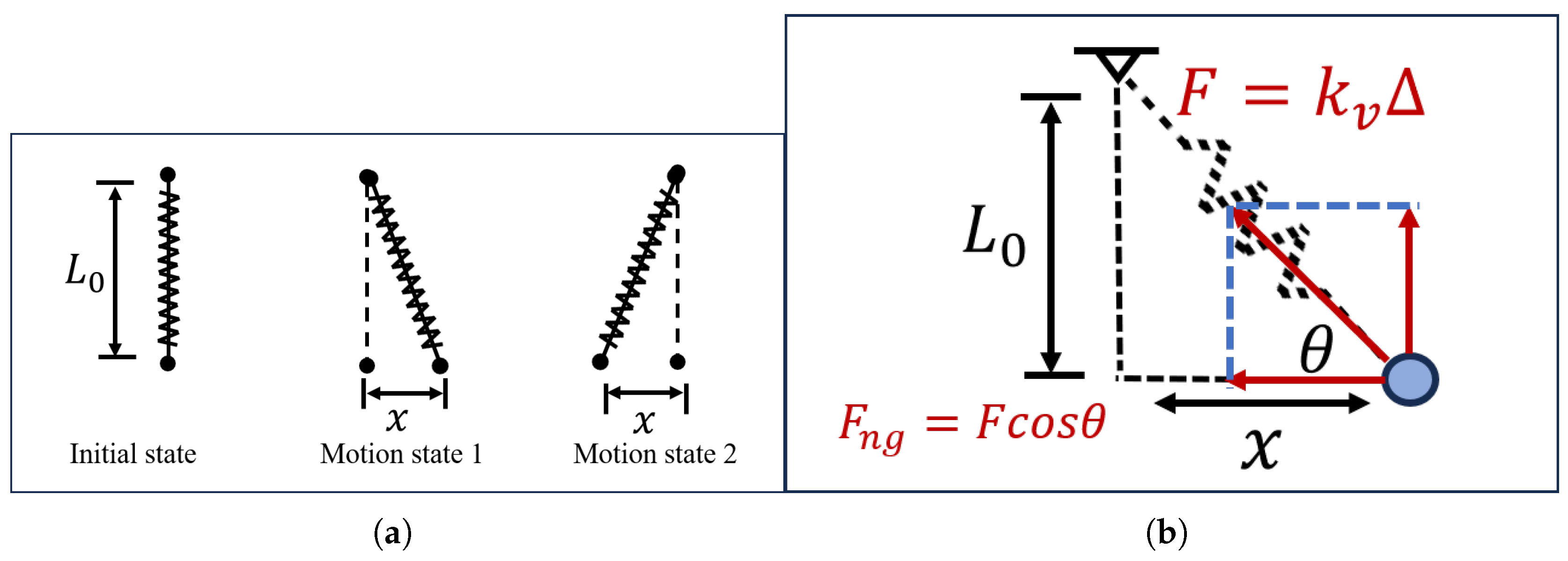
To facilitate a comprehensive understanding of the NSD mechanism, we present a concise introduction to its system architecture in Figure 2. Figure 2 shows the motion state diagram of NSD and the force analysis diagram of NSD.

In Figure 2, the deformation displacement $\Delta$ of the spring is given by the following equation:

$$\Delta =\left|\sqrt{L_0^2+x^2\left(t\right)}-L\right|.$$

(1)

where L and $L_0$ denote the original length and compressed length of the spring, respectively; the spring force $F_{ng}$ can be expressed as follows:

$$F_{ng}=k_{v}x\left(t\right)[{\displaystyle \frac{\Delta }{\sqrt{L_0^2+x^2\left(t\right)}}}]=k_{v}x\left(t\right)[1-L{(L_0^2+x^2\left(t\right))}^{-{\displaystyle \frac{1}{2}}}].$$

(2)

To simplify subsequent calculations, the spring force $F_{ng}$ is expanded using Taylor series:

$${\tilde{F}}_{ng}=k_v\left(1-{\displaystyle \frac{L}{L_0}}\right)x\left(t\right)+{\displaystyle \frac{k_{v}L}{2L_0^3}}{x}^3\left(t\right)-{\displaystyle \frac{3k_{v}L}{8L_0^5}}{x}^5\left(t\right)+{\displaystyle \frac{5k_{v}L}{16L_0^7}}{x}^7\left(t\right)+O\left(x^8\left(t\right)\right).$$

(3)

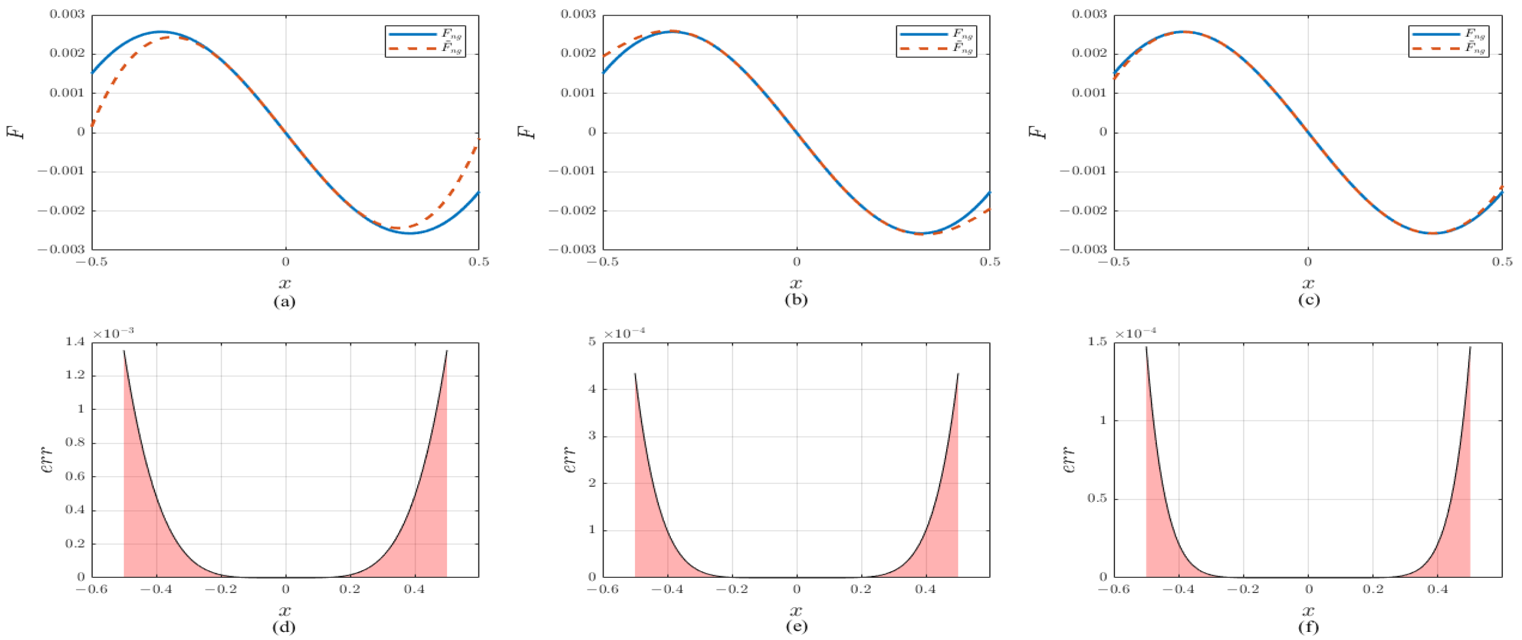
Meanwhile, the absolute error between the Taylor-expanded force ${\tilde{F}}_{ng}$ and the original spring force $F_{ng}$ is calculated using $err=|F_{ng}-{\tilde{F}}_{ng}|.$ Consequently, we obtain the functional plots of Equations (2) and (3) under various Taylor expansion orders, along with their corresponding error distribution diagrams shown in Figure 3.

As illustrated in Figure 3, with the increase in the number of terms in the Taylor series expansion, its approximation accuracy to the original function improves, and the error exhibits a gradual decrease. Furthermore, to investigate the effects of spring stiffness, original length $L_0$, and length L on NSD, we perform first-order differentiation on the original expression Equation (2), then we can obtain the following:

$$K_{nsd}=k_v[1-L{\left(L_0^2+x^2\left(t\right)\right)}^{-{\displaystyle \frac{1}{2}}}]+k_v{x}^2\left(t\right)L{\left(L_0^2+x^2\left(t\right)\right)}^{-{\displaystyle \frac{3}{2}}}.$$

(4)

Therefore, we can obtain the following result plots.

It can be observed from Figure 4 that there is a correlation between the spring stiffness and the negative stiffness provided by NSD: as the spring stiffness gradually increases, the magnitude of the negative stiffness provided by NSD continuously decreases. Meanwhile, the initial spring length also has an impact on the negative stiffness. With the increase in $L_0$, the range of action of the negative stiffness shows a tendency to expand, although the magnitude of the negative stiffness itself also keeps rising. However, from another perspective, when the length of L increases, the negative stiffness will decrease accordingly. Considering all these factors, the initial spring length is a crucial parameter that must be carefully considered in the design and application of negative stiffness devices.

Based on the brief introduction of the NSD system studied in this paper and integrating the analytical frameworks from References [7,32] with Figure 1, we are able to derive the equations of motion that the system follows, as detailed below:

$$m_1\ddot{x}\left(t\right)+(c_1+c_{ng})\dot{x}\left(t\right)+D^{\alpha }x\left(t\right)+k_{1}x\left(t\right)+{\tilde{F}}_{ng}=-m_1{\ddot{x}}_g\left(t\right),$$

(5)

in which, $m_1$ represents the mass of the isolation structure; $c_1$ and $k_1$ are the total damping coefficient and total stiffness coefficient of the isolation bearings, respectively; $c_{ng}$ and $k_v$ correspond to the damping coefficient and negative stiffness coefficient of the negative stiffness device; ${\ddot{x}}_g$ denotes the random excitation; x is the displacement of the isolation structure relative to the ground; $D^{\alpha }x$ represents fractional-order damping. For the convenience of checking the meanings of notations, we have summarized the main notation in Appendix A. Next, we will conduct dimensionless processing on the aforementioned parameters and variables.

$${\omega }_1=\sqrt{{\displaystyle \frac{k_1}{m_1}}},{\xi }_1={\displaystyle \frac{c_1}{2m_1{\omega }_1}},{\xi }_{ng}={\displaystyle \frac{c_{ng}}{2m_1{\omega }_1}},{\alpha }_{ng}={\displaystyle \frac{k_v}{k_1}},{\gamma }_{ng}={\displaystyle \frac{L_0}{L}},{\theta }_{ng}={\displaystyle \frac{{\xi }_{ng}}{{\xi }_1}}.$$

(6)

Based on the aforementioned processing, the dimensionless control equation can ultimately be derived, with its specific form presented as follows:

$$\begin{array}{cc}\hfill & \ddot{x}\left(t\right)+2\left(1+{\theta }_{ng}\right){\xi }_1{\omega }_1\dot{x}\left(t\right)+{\displaystyle \frac{D^{\alpha }}{m_1}}x\left(t\right)+{\omega }_1^2\left(1+{\alpha }_{ng}(1-\frac{1}{{\gamma }_{ng}})\right)x\left(t\right)\hfill \\ \hfill & +{\displaystyle \frac{{\omega }_1^2{\alpha }_{ng}}{2{\gamma }_{ng}{L}_0^2}}{x}^3\left(t\right)-{\displaystyle \frac{3{\omega }_1^2{\alpha }_{ng}}{8{\gamma }_{ng}{L}_0^4}}{x}^5\left(t\right)+{\displaystyle \frac{5{\omega }_1^2{\alpha }_{ng}}{16{\gamma }_{ng}{L}_0^6}}{x}^7\left(t\right)=-{\ddot{x}}_g\left(t\right).\hfill \end{array}$$

(7)

For convenience in subsequent derivation, Equation (7) is now simplified and recorded as follows:

$$\ddot{x}\left(t\right)+h(x\left(t\right),\dot{x}\left(t\right))+{\displaystyle \frac{D^{\alpha }}{m_1}}x\left(t\right)+g\left(x\right)=-{\ddot{x}}_g\left(t\right),$$

(8)

that is

$$h(x\left(t\right),\dot{x}\left(t\right))=2\left(1+{\theta }_{ng}\right){\xi }_1{\omega }_1\dot{x}\left(t\right),$$

(9)

$$g\left(x\right)={\omega }_1^2\left(1+{\alpha }_{ng}(1-{\displaystyle \frac{1}{{\gamma }_{ng}}})\right)x\left(t\right)+{\displaystyle \frac{{\omega }_1^2{\alpha }_{ng}}{2{\gamma }_{ng}{L}_0^2}}{x}^3\left(t\right)-{\displaystyle \frac{3{\omega }_1^2{\alpha }_{ng}}{8{\gamma }_{ng}{L}_0^4}}{x}^5\left(t\right)+{\displaystyle \frac{5{\omega }_1^2{\alpha }_{ng}}{16{\gamma }_{ng}{L}_0^6}}{x}^7\left(t\right).$$

(10)

And the definition of the fractional-order derivative is given as follows:

$$D^{\alpha }x\left(t\right)=\left\{\begin{array}{c}{\displaystyle \frac{1}{\Gamma (n-\alpha )}}{\int }_0^t{\left(\tau \right)}^{n-\alpha -1}{x}^{\left(n\right)}(t-\tau )ds,n-1<\alpha <n\in N\hfill \\ x^{\left(n\right)}\left(t\right),\alpha =n\in N\hfill \end{array}\right..$$

(11)

Here, $\Gamma \left(x\right)$ represents the gamma function, and its specific definition is $\Gamma \left(x\right)={\int }_0^{\infty }{t}^{x-1}{e}^{-t}dt$. What is more, it can be clearly observed from Equation (7) that the system is a random system with a strong nonlinear restoring force and fractional-order damping characteristics. According to the theory of quasi-Hamiltonian system [46], a generalized transformation can be utilized to convert the fast variables $x\left(t\right)$ of the system into slow variables $a\left(t\right),\varphi \left(t\right)$. The transformation equations are as follows:

$$\left\{\begin{array}{c}x\left(t\right)=a\left(t\right)\cos \theta \left(t\right)\hfill \\ \dot{x}\left(t\right)=-a\left(t\right)v(a,\theta )sin\theta \left(t\right)\hfill \\ \theta \left(t\right)=\Phi \left(t\right)+\gamma \left(t\right)\hfill \end{array}\right.,$$

(12)

$$v(a,\theta )={\displaystyle \frac{d\Phi }{dt}}=\sqrt{{\displaystyle \frac{2\left[U\right(a)-U(acos\theta \left)\right]}{a^2{sin}^2\theta }}}=b_0\left(a\right)+\sum _{i=1}^{\infty }{b}_i\left(a\right)\cos i\theta .$$

(13)

In which $U\left(x\right)=\int g\left(x\right)dx$. By integrating $\theta$ in Equation (13) from 0 to $2\pi$, the average frequency of the system can be obtained:

$$\overline{\omega }\left(a\right)=b_0\left(a\right)\triangleq {\overline{\omega }}_a.$$

(14)

Thus, we can obtain the approximate expression of $\theta \left(t\right)$, $\theta \left(t\right)={\overline{\omega }}_{a}t+\gamma \left(t\right)$. Based on the harmonic transformation (12), we can derive the following:

$$\dot{a}cos\theta -\dot{\gamma }sin\theta =0.$$

(15)

In order to obtain the expression of $\ddot{x}\left(t\right)$, we need to differentiate the equation $\dot{x}\left(t\right)=a\left(t\right)v(a,\theta )sin\theta \left(t\right)$ with respect to t, then we have the following:

$$\begin{array}{cc}\hfill \ddot{x}\left(t\right)& =-\dot{a}v(a,\theta )sin\theta \left(t\right)-a{\displaystyle \frac{\partial v(a,\theta )}{\partial a}}\dot{a}sin\theta \left(t\right)-a{\displaystyle \frac{\partial v(a,\theta )}{\partial \theta }}(v(a,\theta )+\dot{\gamma })sin\theta \left(t\right)\hfill \\ \hfill & -a\left(t\right)v(a,\theta )cos\theta \left(t\right)(v(a,\theta )+\dot{\gamma }).\hfill \end{array}$$

(16)

Obviously, to solve the above equation, we must first calculate these two partial derivatives with respect to ${\displaystyle \frac{\partial v(a,\theta )}{\partial a}}$ and ${\displaystyle \frac{\partial v(a,\theta )}{\partial \theta }}$.

$${\displaystyle \frac{\partial v(a,\theta )}{\partial a}}={\displaystyle \frac{\left[g\right(a)-g(a\cos \theta \left)\right]\cos \theta }{a^2{sin}^2\theta v(a,\theta )}}-{\displaystyle \frac{v(a,\theta )}{a}},$$

(17)

$${\displaystyle \frac{\partial v(a,\theta )}{\partial \theta }}={\displaystyle \frac{g\left(a\cos \theta \right)}{a\sin \theta v(a,\theta )}}-{\displaystyle \frac{v(a,\theta )\cos \theta }{\sin \theta }}.$$

(18)

By substituting Equations (17) and (18) into Equation (16) and rearranging, we can obtain the following:

$$\ddot{x}\left(t\right)=-\dot{a}{\displaystyle \frac{\left[g\right(a)-g(a\cos \theta \left)\cos \theta \right]}{a\sin \theta v(a,\theta )}}-g\left(a\cos \theta \right)-\dot{\gamma }{\displaystyle \frac{g\left(a\cos \theta \right)}{v(a,\theta )}}.$$

(19)

Then, taking Equations (12), (15) and (19) into Equation (7), we can derive that

$$\dot{a}={\displaystyle \frac{a\sin \theta v(a,\theta )}{g\left(a\right)}}h(x\left(t\right),\dot{x}\left(t\right))+{\displaystyle \frac{a\sin \theta v(a,\theta )}{g\left(a\right)}}{\displaystyle \frac{D^{\alpha }}{m_1}}x\left(t\right)-{\displaystyle \frac{a\sin \theta v(a,\theta )}{g\left(a\right)}}{\ddot{x}}_g\left(t\right).$$

(20)

$$\dot{\gamma }={\displaystyle \frac{cos\theta v(a,\theta )}{g\left(a\right)}}h(x\left(t\right),\dot{x}\left(t\right))+{\displaystyle \frac{cos\theta v(a,\theta )}{g\left(a\right)}}{\displaystyle \frac{D^{\alpha }}{m_1}}x\left(t\right)-{\displaystyle \frac{cos\theta v(a,\theta )}{g\left(a\right)}}{\ddot{x}}_g\left(t\right)$$

(21)

For the convenience of subsequent derivation and representation, the following notational simplifications are made:

$$\begin{array}{cc}\hfill & F_1={\displaystyle \frac{a\sin \theta v(a,\theta )}{g\left(a\right)}}h(x\left(t\right),\dot{x}\left(t\right))+{\displaystyle \frac{a\sin \theta v(a,\theta )}{g\left(a\right)}}{\displaystyle \frac{D^{\alpha }}{m_1}}x\left(t\right),G_1=-{\displaystyle \frac{a\sin \theta v(a,\theta )}{g\left(a\right)}},\hfill \\ \hfill & F_2={\displaystyle \frac{cos\theta v(a,\theta )}{g\left(a\right)}}h(x\left(t\right),\dot{x}\left(t\right))+{\displaystyle \frac{cos\theta v(a,\theta )}{g\left(a\right)}}{\displaystyle \frac{D^{\alpha }}{m_1}}x\left(t\right),G_2=-{\displaystyle \frac{cos\theta v(a,\theta )}{g\left(a\right)}}.\hfill \end{array}$$

(22)

At this point, based on the stochastic averaging procedure [47], we can derive the following $It\widehat{o}$ stochastic differential equation.

$$da=m\left(a\right)dt+\sigma \left(a\right)dB\left(t\right),$$

(23)

$$m\left(a\right)={\langle F_1+D{\displaystyle \frac{\partial G_1}{\partial a}}{G}_1+D{\displaystyle \frac{\partial G_1}{\partial \gamma }}{G}_2\rangle }_{\theta },$$

(24)

$${\sigma }^2\left(a\right)={\langle 2D{G}_1^2\rangle }_{\theta }={\displaystyle \frac{D{a}^2{v}^2(a,\theta )}{g{\left(a\right)}^2}}.$$

(25)

The process undergone by the variable $\theta \left(t\right)$ is a slow-varying process. Thus, the Taylor expansion can be performed on it, leading to the following result:

$$\theta (t-\tau )=\theta \left(t\right)-\overline{\omega }\left(a\right)\tau .$$

(26)

Based on this, we proceed to calculate the time-averaged expressions for the drift coefficient and the diffusion coefficient, with the specific calculation process as follows. First, we perform time-averaging calculations on the fractional derivative part:

$$\begin{array}{cc}\hfill & {\langle {\displaystyle \frac{a\sin \theta v(a,\theta )}{g\left(a\right)}}{\displaystyle \frac{D^{\alpha }}{m_1}}x\left(t\right)\rangle }_{\theta }={\displaystyle \frac{1}{g\left(a\right)m_1}}\underset{T\to \infty }{lim}{\displaystyle \frac{1}{T}}{\int }_0^T{D}^{\alpha }\left(a\cos \theta \right)a\sin \theta v(a,\theta )dt\hfill \\ \hfill & ={\displaystyle \frac{1}{g\left(a\right)m_1}}\underset{T\to \infty }{lim}{\displaystyle \frac{1}{T\Gamma (1-\alpha )}}{\int }_0^T\left({\int }_0^t{\displaystyle \frac{x^{\prime }(t-\tau )}{{\tau }^{\alpha }}}d\tau \right)a\sin \theta v(a,\theta )dt\hfill \\ \hfill & ={\displaystyle \frac{1}{\Gamma (1-\alpha )g\left(a\right)m_1}}\underset{T\to \infty }{lim}{\displaystyle \frac{1}{T}}{\int }_0^{T}a\sin \theta v(a,\theta )d\left({\int }_0^t{\displaystyle \frac{x(t-\tau )}{{\tau }^{\alpha }}}d\tau \right)\hfill \\ \hfill & ={\displaystyle \frac{1}{\Gamma (1-\alpha )g\left(a\right)m_1}}\underset{T\to \infty }{lim}\{{\displaystyle \frac{1}{T}}a\sin \theta v(a,\theta ){\int }_0^t{\displaystyle \frac{x(t-\tau )}{{\tau }^{\alpha }}}d\tau {|}_0^T\hfill \\ \hfill & -{\displaystyle \frac{1}{T}}{\int }_0^T\left({\int }_0^t{\displaystyle \frac{x(t-\tau )}{{\tau }^{\alpha }}}d\tau \right){\displaystyle \frac{d\left(a\sin \theta v\right(a,\theta \left)\right)}{dt}}dt\}.\hfill \end{array}$$

(27)

From the existing literature [48], we can obtain the following expression:

$${\int }_0^t{\displaystyle \frac{sin\left({\overline{\omega }}_{a}s\right)}{s^{\alpha }}}ds={\overline{\omega }}_a^{\alpha -1}[\Gamma (1-\alpha )cos{\displaystyle \frac{\pi \alpha }{2}}-{\displaystyle \frac{cos{\omega }_{1}t}{{\left({\omega }_{1}t\right)}^{\alpha }}}+o{\left({\omega }_{1}t\right)}^{-\alpha }],$$

(28)

$${\int }_0^t{\displaystyle \frac{cos\left({\overline{\omega }}_{a}s\right)}{s^{\alpha }}}ds={\overline{\omega }}_a^{\alpha -1}[\Gamma (1-\alpha )sin{\displaystyle \frac{\pi \alpha }{2}}-{\displaystyle \frac{sin{\omega }_{1}t}{{\left({\omega }_{1}t\right)}^{\alpha }}}+o{\left({\omega }_{1}t\right)}^{-\alpha }].$$

(29)

By using Equations (28) and (29), we can derive that

$$\begin{array}{cc}\hfill & \underset{T\to \infty }{lim}{\displaystyle \frac{1}{T}}a\sin \theta v(a,\theta ){\int }_0^t{\displaystyle \frac{x(t-\tau )}{{\tau }^{\alpha }}}{d\tau |}_0^T\hfill \\ \hfill & \approx \underset{T\to \infty }{lim}{\displaystyle \frac{1}{T}}(av(a,\theta )\sin \theta \cos \theta {\int }_0^T{\displaystyle \frac{cos\left({\overline{\omega }}_a\tau \right)}{{\tau }^{\alpha }}}d\tau +av(a,\theta ){\sin }^2\theta {\int }_0^T{\displaystyle \frac{sin\left({\overline{\omega }}_a\tau \right)}{{\tau }^{\alpha }}}d\tau )\hfill \\ \hfill & \approx \underset{T\to \infty }{lim}{\displaystyle \frac{av(a,\theta )\sin \theta {\overline{\omega }}_a^{\alpha -1}}{T}}(\Gamma (1-\alpha )sin(\theta +{\displaystyle \frac{\alpha \pi }{2}})+{\displaystyle \frac{sin({\omega }_{1}T-\theta )}{{({\omega }_{1}T)}^{\alpha }}})=0.\hfill \end{array}$$

(30)

By substituting the conclusion derived from Equation (30) into Equation (27), we can further deduce:

$$\begin{array}{cc}\hfill & {\langle {\displaystyle \frac{a\sin \theta v(a,\theta )}{g\left(a\right)}}{\displaystyle \frac{D^{\alpha }}{m_1}}x\left(t\right)\rangle }_{\theta }\hfill \\ \hfill & =-{\displaystyle \frac{1}{g\left(a\right)m_1\Gamma (1-\alpha )}}\underset{T\to \infty }{lim}{\displaystyle \frac{1}{T}}{\int }_0^{T}ag\left(a\cos \theta \right)[\cos \theta {\int }_0^t{\displaystyle \frac{\cos {\overline{\omega }}_a\tau }{{\tau }^{\alpha }}}d\tau +\sin \theta {\int }_0^t{\displaystyle \frac{\sin {\overline{\omega }}_a\tau }{{\tau }^{\alpha }}}d\tau ]dt\hfill \\ \hfill & \approx -{\displaystyle \frac{a}{g\left(a\right)m_{1}2\pi {\overline{\omega }}_a^{1-\alpha }}}{\int }_0^{2\pi }g\left(a\cos \theta \right)[\cos \theta sin\left({\displaystyle \frac{\alpha \pi }{2}}\right)+\sin \theta cos\left({\displaystyle \frac{\alpha \pi }{2}}\right)d\theta ].(0<\alpha <1)\hfill \end{array}$$

(31)

In Equation (13), $U\left(x\right)$ represents the system’s energy, and its specific expression is as follows:

$$\begin{array}{cc}\hfill & U\left(x\right)\hfill \\ & =\int {\omega }_1^2(1+{\alpha }_{ng}(1-{\displaystyle \frac{1}{{\gamma }_{ng}}}))x\left(t\right)+{\displaystyle \frac{{\omega }_1^2{\alpha }_{ng}}{2{\gamma }_{ng}{L}_0^2}}{x}^3\left(t\right)-{\displaystyle \frac{3{\omega }_1^2{\alpha }_{ng}}{8{\gamma }_{ng}{L}_0^4}}{x}^5\left(t\right)+{\displaystyle \frac{5{\omega }_1^2{\alpha }_{ng}}{16{\gamma }_{ng}{L}_0^6}}{x}^7\left(t\right)dx\hfill \\ \hfill & ={\displaystyle \frac{1}{2}}{\omega }_1^2(1+{\alpha }_{ng}(1-{\displaystyle \frac{1}{{\gamma }_{ng}}}))x{\left(t\right)}^2+{\displaystyle \frac{{\omega }_1^2{\alpha }_{ng}}{8{\gamma }_{ng}{L}^2}}{x}^4\left(t\right)-{\displaystyle \frac{3{\omega }_1^2{\alpha }_{ng}}{48{\gamma }_{ng}{L}_0^4}}{x}^6\left(t\right)+{\displaystyle \frac{5{\omega }_1^2{\alpha }_{ng}}{128{\gamma }_{ng}{L}_6^6}}{x}^8\left(t\right)\hfill \\ \hfill & \triangleq {\displaystyle \frac{1}{2}}K{x}^2\left(t\right)+{\displaystyle \frac{1}{4}}{K}_2{x}^4\left(t\right)-{\displaystyle \frac{1}{6}}{K}_3{x}^6\left(t\right)+{\displaystyle \frac{1}{8}}{K}_4{x}^8\left(t\right),\hfill \end{array}$$

(32)

in which, $K={\omega }_1^2+{\omega }_1^2{\alpha }_{ng}(1-{\displaystyle \frac{1}{{\gamma }_{ng}}})$, $K_2={\displaystyle \frac{{\omega }_1^2{\alpha }_{ng}}{2{\gamma }_{ng}{L}_3^2}}$, $K_3={\displaystyle \frac{3{\omega }_1^2{\alpha }_{ng}}{8{\gamma }_{ng}{L}_0^4}}$, $K_4={\displaystyle \frac{5{\omega }_1^2{\alpha }_{ng}}{16{\gamma }_{ng}{L}_0^6}}$. Thus, by using Equation (13), we can calculate the expression of $v(a,\theta )$.

$$\begin{array}{cc}\hfill v(a,\theta )& =\sqrt{{\displaystyle \frac{2[\frac{1}{2}K(a^2-a^2{cos}^2\theta )+\frac{1}{4}{K}_2(a^4-a^4{cos}^4\theta )-\frac{1}{6}{K}_3(a^6-a^6{cos}^6\theta )+\frac{1}{8}{K}_4(a^8-a^8{cos}^8\theta )]}{a^2{sin}^2\theta }}}\hfill \\ \hfill & =\sqrt{K+{\displaystyle \frac{K_2{a}^2(1+{cos}^2\theta )}{2}}-{\displaystyle \frac{K_3{a}^4(1+{cos}^2\theta +{cos}^4\theta )}{3}}+{\displaystyle \frac{K_4{a}^6(1+{cos}^2\theta )(1+{cos}^4\theta )}{4}}}\hfill \\ \hfill & ={\left[\eta (1+{\eta }_{1}cos2\theta +{\eta }_{2}cos4\theta +{\eta }_{3}cos6\theta )\right]}^{{\displaystyle \frac{1}{2}}}\hfill \\ \hfill & \approx b_0\left(a\right)+b_2\left(a\right)cos2\theta +b_4\left(a\right)cos4\theta +b_6\left(a\right)cos6\theta .\hfill \end{array}$$

(33)

The full derivation is shown in Appendix B.1. Thus, we can obtain the average frequency ${\overline{\omega }}_a=b_0\left(a\right)$. Now, we define ${\overline{\omega }}_a\triangleq v$. Based on this definition, we are able to carry out the subsequent calculations of the drift function and the diffusion function and obtain the corresponding results:

$$\begin{array}{cc}\hfill m\left(a\right)& ={\langle F_1+D{\displaystyle \frac{\partial G_1}{\partial a}}{G}_1+D{\displaystyle \frac{\partial G_1}{\partial \gamma }}{G}_1+D{\displaystyle \frac{\partial G_1}{\partial \gamma }}{G}_2\rangle }_{\theta }\hfill \\ \hfill & =-{\displaystyle \frac{{\left(av\right)}^2}{g\left(a\right)}}\left((1+{\theta }_{ng}){\xi }_1{\omega }_1\right)-{\displaystyle \frac{a(\frac{Ka}{8}+\frac{3}{8}{K}_2{a}^3-\frac{5}{16}{K}_3{a}^5+\frac{35}{128}{K}_4{a}^7)}{g\left(a\right)m_1{\overline{\omega }}_a^{1-\alpha }}}\hfill \\ \hfill & +D[{\displaystyle \frac{a^{2}v{v}^{\prime }}{2g{\left(a\right)}^2}}+{\displaystyle \frac{a{v}^2}{g{\left(a\right)}^2}}-{\displaystyle \frac{a^2{v}^2{g}^{\prime }\left(a\right)}{2g{\left(a\right)}^3}}].\hfill \end{array}$$

(34)

$${\sigma }^2\left(a\right)={\langle 2D{G}_1^2\rangle }_{\theta }={\displaystyle \frac{D{a}^2{v}^2}{g{\left(a\right)}^2}}.$$

(35)

And the related expressions are shown in Appendix B.2:

3. Reliability Index and Associated Equations

Suppose the safety range of the system’s amplitude is defined by the closed interval $\Omega =[0,a]\in R$. Under this assumption, the time-varying reliability function $R\left(t\right|a_0,L_0)$ can be defined as the probability that, when the system’s initial amplitude is $a_0\in \Omega$, the system’s amplitude remains within the safety domain $\Omega$ after a time period $t\in (0,T]$.

$$R\left(t\right|a_0,L_0)=p\{a_0\left(t\right)\in \Omega ,t\in (0,T]|a_0\left(t\right)\in \Omega \}.$$

(36)

To derive the differential equation satisfied by $R\left(t\right|a_0,L_0)$, we introduce the conditional transition probability density $q(a,t|a_0,L_0)$. This conditional transition probability density describes the transition probability density of sample functions for which the system process remains consistently within the safety domain $\Omega$ over the time interval $(0,T]$, and it satisfies the Backward Kolmogorov (BK) equation [49]:

$${\displaystyle \frac{\partial q(a,t|a_0,L_0)}{\partial t}}={\mathcal{L}}_{BK}\left[q(a,t|a_0,L_0)\right],$$

(37)

${\mathcal{L}}_{BK}$ is an elliptic operator, and its specific expression is as follows:

$${\mathcal{L}}_{B\mathcal{K}}=m\left(a_0\right){\displaystyle \frac{\partial }{\partial a_0}}+{\displaystyle \frac{1}{2}}{\sigma }^2\left(a_0\right){\displaystyle \frac{{\partial }^2}{\partial a_0^2}}.$$

(38)

As demonstrated by the formulas presented earlier, the expressions for $m\left(a_0\right)$ and ${\sigma }^2\left(a_0\right)$ have been clearly given. The conditional reliability function refers to the proportion of the number of samples for which the system remains consistently within the safety domain $\Omega$ over the time interval $[0,T]$ to the total number of samples. Therefore, we can obtain the following:

$$R\left(t\right|a_0,\tau )={\int }_{\Omega }q(a,t|a_0,L_0)da.$$

(39)

By performing the integration operation on both sides of the equation with respect to the variable a over the safety domain $\Omega$, we can derive that the time-varying reliability function $R\left(t\right|a_0,L_0)$ satisfies the BK equation, and this equation is a parabolic backward partial differential equation.

$${\displaystyle \frac{\partial R\left(t\right|a_0,L_0)}{\partial t}}=m\left(a_0\right){\displaystyle \frac{\partial }{\partial a_0}}R\left(t\right|a_0,L_0)+{\displaystyle \frac{1}{2}}{\sigma }^2\left(a_0\right){\displaystyle \frac{{\partial }^2}{\partial a_0^2}}R\left(t\right|a_0,L_0).$$

(40)

Moreover, this equation is required to satisfy the following initial and boundary conditions:

$$\begin{array}{c}R\left(0\right|a_0,L_0)=1,a_0\in \Omega \hfill \\ \left\{\begin{array}{c}R\left(t\right|a_0,L_0)=p_1,a_0=0\hfill \\ R\left(t\right|a_0,L_0)=0,a_0\in \partial \Omega \hfill \end{array}\right..\hfill \end{array}$$

(41)

Here, $p_1$ is a probability constant, and it satisfies $0\le p_1\le 1$. Meanwhile, for the probability $p_T\left(t\right|a_0,L_0)$ regarding the first-passage time, there exists the following calculation expression:

$$p_T\left(t\right|a_0,L_0)=-{\displaystyle \frac{\partial R\left(t\right|a_0,L_0)}{\partial t}}{|}_{t=T\left(a_0\right)}.$$

(42)

4. Optimization Problem Formulation and PSO-GRBFNN Algorithm Framework

This paper aims to achieve the highest possible level of system reliability by solving for the optimal system parameters. Thus, the following reliability optimization problem is established:

$${\displaystyle max\underset{L_0}{arg}R\left(t\right|a_0,L_0),t\in [0,T]}$$

(43)

$$\begin{array}{c}s.t.\left\{\begin{array}{c}{\displaystyle \frac{\partial }{\partial t}R\left(t\right|a_0,L_0)={\mathcal{L}}_{\mathcal{BK}}\left[R\left(t\right|a_{10},L_0)\right]}\hfill \\ R\left(t\right|a_{10},L_0)=p_1,a_{10}=0\hfill \\ R\left(t\right|a_{10},L_0)=0,a_{10}\in \partial \Omega \hfill \\ R\left(0\right|a_{10},L_0)=1,a_{10}\in \Omega \hfill \end{array}\right.\hfill \end{array}$$

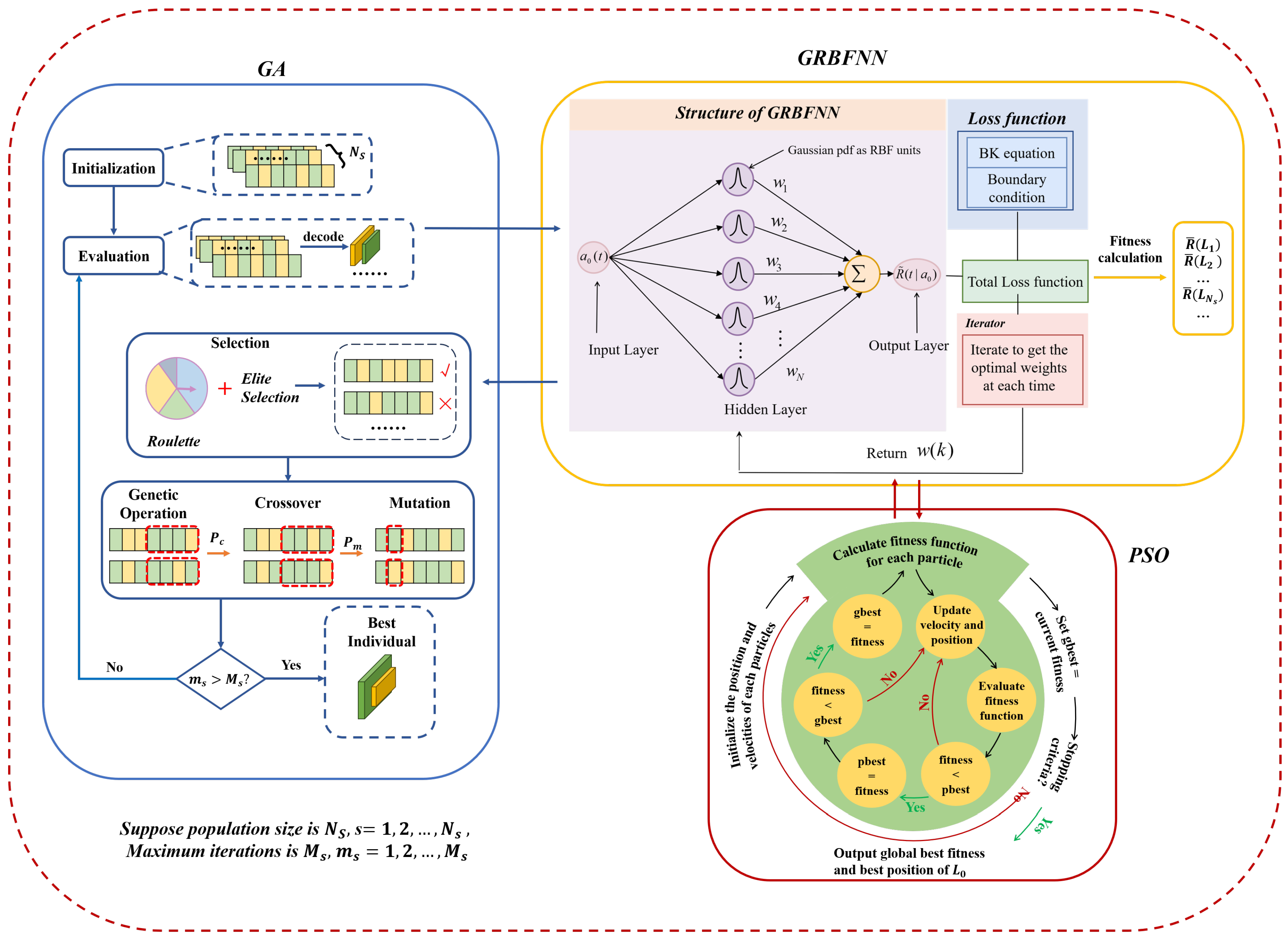
In the formulated optimization problem, the parameter $L_0$ is unknown and its value needs to be determined by maximizing the reliability function. Moreover, this process is subject to the constraints imposed by the BK equation, along with its corresponding initial and boundary conditions. In this problem, the objective function exhibits a non-explicit characteristic, and its solution is highly dependent on the solution of the BK equation. Given that conventional optimization algorithms struggle to tackle such complex problems, in previous research, we proposed the use of the GA-GRBFNN algorithm to address this issue [45]. Although the GA-GRBFNN algorithm can effectively handle the problem, as the number of iterations increases and the population size expands, its operational efficiency gradually declines and its performance becomes sluggish. Based on this, this paper proposes the PSO-GRBFNN algorithm to overcome the aforementioned difficulties. The overall framework and ideas of the two algorithms are shown in Figure 5.

As can be seen from Figure 5, the GRBFNN algorithm serves as the core part of these two algorithms, undertaking the task of calculating the fitness function. Moreover, compared with the GA algorithm, the PSO algorithm has a simpler overall process and requires the generation of a relatively smaller amount of data. Since the GA-GRBFNN algorithm has been elaborated in detail in previous studies, this paper will focus on elaborating the process of the PSO-GRBFNN algorithm.

Step 1: Initialization

Within the domain of definition of $L_0$, randomly generate the initial position set $X=(X_1,X_2,\dots ,X_{N_s})$ and the initial velocity set $V=(V_1,V_2,\dots ,V_{N_s})$ for $N_s$ particles. Meanwhile, record the current individual position of each particle as its individual best position $P_b$, and randomly select the best position from all particles as the initial global best position $G_b$.

Step 2: Fitness Function Design

The selection of the fitness function plays a critically decisive role in the performance of the PSO algorithm. Meanwhile, the complexity of the fitness function also impacts the complexity of the algorithm. In the PSO-GRBFNN algorithm, this research innovatively embeds the GRBFNN into the PSO framework to calculate the fitness function for each particle. During each iteration of the algorithm, PSO and GRBFNN work in close collaboration in a coupled manner. This improvement represents the most innovative core idea in our research work, aiming to effectively address the challenge of non-explicit expression of the objective function. Given that the reliability function has the characteristic of non-negativity and GRBFNN possesses the ability to solve the BK equation, we select the reliability function value calculated by GRBFNN as the fitness function value. When adopting this method, we need to make the following assumptions:

$$\tilde{R}\left(t_k\right|a_0,w\left(t_k\right))=\sum _{i=1}^N{w}_i\left(t_k\right)G(a_0,u_i,{\sigma }_i),(k=1,2,\dots )$$

(44)

$w\left(t_k\right)={[w_1\left(t_k\right),w_2\left(t_k\right),\dots w_N\left(t_k\right)]}^T$ represents the weight coefficient vector to be determined, where $w_i\left(t_k\right)$ denotes the weight coefficient corresponding to the i-th kernel function at the k-th step. What is more, the kernel functions of GRBFNN are Gaussian functions, and a weighted sum of N kernel functions is employed to approximate the solution of the original equation. For the i-th kernel function, its mean and variance are given by ${\mu }_i={\displaystyle \frac{(i-\frac{1}{2})\partial \Omega }{N}}$ and ${\sigma }_i={\displaystyle \frac{\partial \Omega }{N}}$, respectively. The specific expression of the Gaussian kernel function is as follows:

$$G(a_0,{\mu }_i,{\sigma }_i)=\prod _{j=1}^2{\displaystyle \frac{1}{\sqrt{2\pi }{\sigma }_i}}exp\left({\displaystyle \frac{{\left({a_0}_j-{\mu }_{ij}\right)}^2}{2{\sigma }_i^2}}\right).$$

(45)

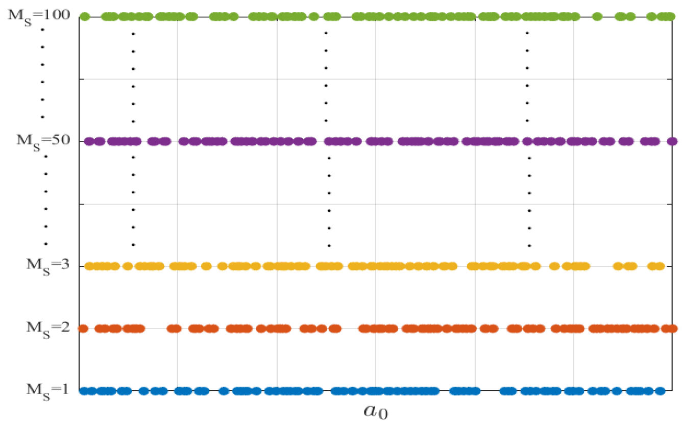
The initial amplitude serves as the sole input variable in the GRBFNN structure. Consequently, we only need to generate training data of size M for each iteration of PSO. Thus, the overall size of the training data is $M_s\ast M$. The training data are generated through uniform sampling within the defined domain. This method can effectively avoid the phenomenon of data clustering, ensuring the uniformity and rationality of data distribution. Additionally, the training data we generated are shown in Figure 6.

Furthermore, based on the findings in paper [31], the size of the training data should be at least four times the number of neurons, i.e., $M=4N$. Using these training data, each set is fed into the neural network. In the neural network, by substituting the approximate solution into Equation (40) the BK operator, we can obtain the error, denoted as $Er{r}_1(a_0,w\left(t_k\right))$, between the exact solution and the approximate solution of the system.

$$\begin{array}{c}Er{r}_1(a_0,w\left(t_k\right))=\Delta t\times {\mathcal{L}}_{BK}\left[\tilde{R}\left(t_k\right|a_0,w\left(t_k\right))\right]-\tilde{R}\left(t_k\right|a_0,w\left(t_k\right))+\tilde{R}\left(t_k\right|a_0,w\left(t_{k-1}\right))\\ ={\displaystyle \sum _{i=1}^N}{w}_i\left(t_k\right)h_i\left(a_0\right)+{\displaystyle \sum _{i=1}^N}{w}_i\left(t_{k-1}\right)G(a_0,{\mu }_i,{\sigma }_i).\end{array}$$

(46)

where $\Delta t$ represents the time step, and $h_i\left(a_0\right)=\Delta t\times {\mathcal{L}}_{BK}\left[G(a_0,{\mu }_i,{\sigma }_i)\right]-G(a_0,{\mu }_i,{\sigma }_i)$. Additionally, the reliability function satisfies specific boundary conditions. Consequently, a second component is incorporated into the loss function to fulfill this requirement.

$$Er{r}_2(a_0,w\left(t_k\right))=\tilde{R}\left(t_k\right|a_0,w\left(t_k\right))-\partial \Omega$$

(47)

Therefore, the loss function associated with the solution of the BK equation should account for both the local error and the boundary condition simultaneously. Based on this, we construct the loss function as follows:

$$Los{s}_{\left[BK\right]}[w\left(t_k\right),\lambda \left(t_k\right)]={\displaystyle \frac{1}{2}}{\int }_{\Omega }{\left[Er{r}_1(a_0,w\left(t_k\right))\right]}^{2}d{a}_0+{\displaystyle \frac{1}{2}}\lambda \left(t_k\right){\int }_{\partial \Omega }[Er{r}_2(a_0,w\left(t_k\right))-\partial \Omega ]d{a}_0$$

(48)

Here, $\lambda \left(t_k\right)$ is the Lagrange multiplier to be determined, $\Omega$ represents the safe domain for the variable $a_0$, and $\partial \Omega$ denotes the boundary of this safe domain. Subsequently, based on the partition of the safe domain, we can discretize the loss function as follows:

$$\begin{array}{cc}\hfill & {\displaystyle Los{s}_{\left[BK\right]}[w\left(t_k\right),\lambda \left(t_k\right)]}\hfill \\ \hfill & {\displaystyle =\frac{1}{2}\sum _{j=1}^M\left(\sum _{i=1}^N\sum _{l=1}^N{h}_i\left(a_{0j}\right)h_l\left(a_{0j}\right)w_i\left(t_k\right)w_l\left(t_k\right)\right)+\sum _{j=1}^M\sum _{i=1}^N{h}_i\left(a_{0j}\right)w_i\left(t_k\right)\tilde{R}\left(t_k\right|a_{0j},w\left(t_k\right))}\hfill \\ \hfill & {\displaystyle +\frac{1}{2}\sum _{j=1}^M\tilde{R}{\left(t_{k-1}\right|a_{0j},w\left(t_{k-1}\right))}^2+\lambda \left(t_k\right)\sum _{j=1}^{M_2}\tilde{R}\left(t_{k-1}\right|a_{0j},w\left(t_{k-1}\right))}\hfill \\ \hfill & {\displaystyle =\frac{1}{2}{w}^T\left(t_k\right)[H_0+\lambda \left(t_k\right)R_b]w\left(t_k\right)+w^T\left(t_k\right)Q_{0}w\left(t_{k-1}\right)+d_0\left(t_{k-1}\right).}\hfill \end{array}$$

(49)

In which $G_1={\left[G_{ij}\right]}_1=\left[G(a_{0j},{\mu }_i,{\sigma }_i)\right],{\tilde{a}}_{0j}\in \partial \Omega ,H=\left[h_i\left(a_{0j}\right)\right],H_0=H{H}^T,$ $Q_0=H{G}^T,R_b=G_1{G}_1^T,d_0\left(t_{k-1}\right)={\displaystyle \frac{1}{2}}{w}^T\left(t_{k-1}\right)$. To minimize the error of the solution obtained by the neural network under the control of parameters $w\left(t_k\right),\lambda \left(t_k\right)$, the following conditions need to be satisfied:

$$\left\{\begin{array}{c}{\displaystyle \frac{\partial Los{s}_{\left[BK\right]}\left[w\left(t_k\right),\lambda \left(t_k\right)\right]}{\partial w\left(t_k\right)}}=0,\hfill \\ {\displaystyle \frac{\partial Los{s}_{\left[BK\right]}\left[w\left(t_k\right),\lambda \left(t_k\right)\right]}{\partial \lambda \left(t_k\right)}}=0,\hfill \end{array}\right.$$

(50)

By solving Equation (50), we can derive an iterative formula for the unknown weighted coefficients $w\left(t_k\right)$, as detailed below:

$$w\left(t_k\right)=Zl\left(t_k\right)$$

(51)

$$l\left(t_k\right)=-{\left(Z^T{H}_{0}Z\right)}^{-1}\left(Z^T{Q}_{0}Z\right)l\left(t_{k-1}\right)$$

(52)

Among them, Z belongs to the null subspace of $R_b$. Subsequently, based on the neural network constructed with the aforementioned weights, we can obtain the time-varying reliability functions. In this paper, we adopt the average reliability function value corresponding to each parameter to be optimized as the fitness function value for GA.

$$\overline{R}\left(\tau \right)={\displaystyle \frac{1}{T}}\sum _{k=1}^{\left[{\displaystyle \frac{T}{\Delta t}}\right]}R\left(t_k\right|a_0),\tau =\left({\tau }_1,{\tau }_2\cdots {\tau }_{N_s}\right).$$

(53)

Step 3: Iterative Update

Update of the individual best position $P_b$: If the fitness value corresponding to the current particle is superior to the particle’s current individual best fitness value, then update the individual best value of this particle. The specific update rules are as follows:

$$P_{i_b}=\left\{\begin{array}{c}{P}_{i_b}\overline{R}\left(L_{0_i}\right)<\overline{R}\left(P_{i_b}\right)\hfill \\ L_{0_i}\overline{R}\left(L_{0_i}\right)\ge \overline{R}\left(P_{i_b}\right)\hfill \end{array}\right..$$

(54)

Update of the global best position $G_b$: If there exists a particle in the current particle swarm whose fitness value is superior to the currently recorded optimal fitness value of the entire swarm, then update the global best value of the current particle swarm. The specific update rules are as follows:

$$G_b=\left\{\begin{array}{c}{P}_{i_b}\overline{R}\left(P_{i_b}\right)\ge G_b\hfill \\ G_b\overline{R}\left(P_{i_b}\right)<G_b\hfill \end{array}\right..$$

(55)

Update of velocity and position:

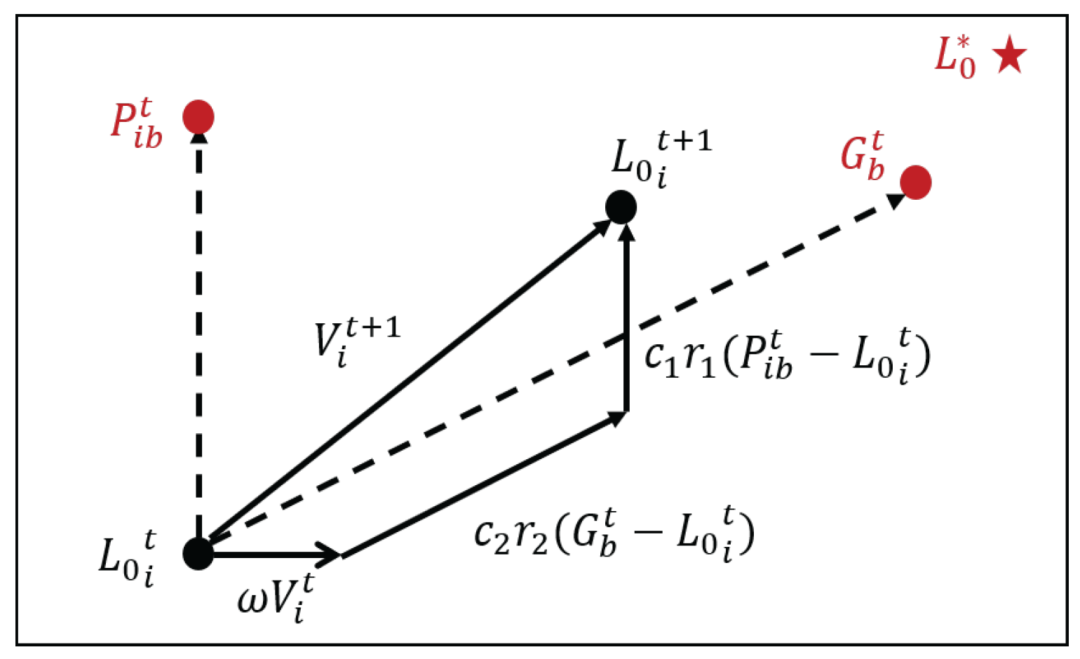
Regarding the two crucial parameters of velocity and position, their update process can be referred to in Figure 7.

By observing this figure, it can be clearly seen that the iterative calculations for velocity and position follow the following formulas:

$$\begin{array}{c}{V}_i^{t+1}=\omega V_i^t+c_1{r}_1(P_{i_b}^t-L_{0_i}^t)+c_2{r}_2(G_b^t-L_{0_i}^t),\hfill \\ {L_0}_i^{t+1}={L_0}_i^t+V_i^{t+1}.\hfill \end{array}$$

(56)

Here, $\omega$ is the inertia weight, which is used to regulate the extent to which a particle inherits its previous velocity. $r_1$ and $r_2$ are random numbers within the range of $[0,1]$. $c_1$ and $c_2$ are learning factors that adjust the influence of individual experience and swarm experience on particle updates, with their values typically falling between 1 and 2.

In the iterative formula, the first part is the memory term, which generally reflects the impact of a particle’s previous velocity magnitude and direction on its current velocity. The second term is called the self-cognition term. It is a vector pointing from the current point to the particle’s own historical best position, representing the change trend of the particle based on its own experience. The third term is referred to as the swarm cognition term. It is a vector pointing from the current point to the global best position of the swarm, reflecting how particles adjust their states through collaboration and knowledge sharing. Particles determine their next move by comprehensively considering both their own experience and the swarm’s experience.

At this point, the particle swarm algorithm has completed one round of iteration, and the position parameters and velocity parameters $(L_0,V)$ are updated. Subsequently, the process repeats from Step 2 to Step 3 to continuously update and optimize the parameters. Eventually, the optimal control parameters that maximize the reliability function can be obtained. Algorithm 1 presents the pseudocode for the PSO-GRBFNN algorithm.

Algorithm 1 PSO-GRBFNN Algorithm

Require:  Size of the particle swarm $N_S$, Maximum iteration times for the PSO $M_S$, Value range of $L_0$, Inertia weight $\omega$, Learning factors $c_1$ and $c_2$, Random parameters $r_1$ and $r_2$ within the range $[0,1]$, Number of Gaussian radial basis functions N. Ensure:  The optimal values $L_0^{*}$ and $\overline{R}$.   1: Generating an initial population of size $N_S$, setting the initial value of $L_0$ and the velocity V.   2: Setting the initial individual historical best position $P_b$ and the global historical best position $G_b$.   3: while iteration times $<M_S$ do   4:   Generating training data associated with amplitude a   5:   Employing the GRBFNN method to obtain the weights $\omega \left(t_k\right)$   6:   Calculating the corresponding reliability values for each particle   7:   Updating $P_b$ and $G_b$ based on the fitness function values of each particle.   8:   Updating particle positions $L_0$ and velocities V using iterative formulas.   9: end while 10: Selecting the particle with the best fitness as $G_b$ a 11: return optimal $L_0^{*}$ and $\overline{R}$.

To facilitate a comparative analysis between the PSO-GRBFNN algorithm and the GA-GRBFNN algorithm, Algorithm 2 provides a systematic summary of the pseudocode for the GA-GRBFNN algorithm.

Algorithm 2 GA-GRBFNN Algorithm

Require:  Size of the population $N_S$, Maximum generations for the GA $M_S$, Value range of $L_0$, Crossover probability $P_c$, Mutation probability $P_m$, Roulette probability $P_s$, Number of Gaussian radial basis functions N. Ensure:  The optimal values $L_0^{*}$ and $\overline{R}$.   1: Generating an initial population size $N_S$, setting the initial values for the parameters $L_0$ in binary format   2: while iteration times $<M_S$ do   3:   Generating training data associated with amplitude a   4:   Employing the GRBFNN method to obtain the weights $\omega \left(t_k\right)$   5:   Calculating the corresponding reliability values for each individual   6:   Evaluating the fitness function $\overline{R}\left(L_0\right)$ for each individual within the population   7:   Conducting selection based on an improved roulette wheel selection strategy   8:   Performing arithmetic crossover to generate offspring with probability $P_c$   9:   Applying mutation to introduce minor changes with probability $P_m$ 10: end while 11: Selecting the individual with the best fitness as the optimal solution 12: Extracting the optimal $L_0$ values from the optimal individual 13: return Optimal $L_0^{*}$ and $\overline{R}$.

5. Numerical Simulation

In this section, we employ the GA-GRBFNN algorithm and the PSO-GRBFNN algorithm to conduct exploratory research on the optimal reliability probability of the system. Meanwhile, we utilize the Monte Carlo simulation method to comparatively validate the effectiveness and accuracy of these two proposed algorithms and engage in an in-depth discussion on their performance.

Under the given parameter conditions where ${\omega }_1=2,{\gamma }_{ng}=0.6,L=1,\theta =1,$ $\xi =0.15,$ $m_1=4,700,000,\alpha =0.5,$ and $D=0.5$, through calculations using the GA-GRBFNN algorithm with $N_S=80,M_S=100,P_c=0.6,P_m=0.005$ and $ϵ=0.0001$, we can obtain $L_0=0.66795$; by employing the PSO-GRBFNN algorithm with $N_S=20,M_S=50,$ $c_1=1.5,$ $c_2=1.5,\omega =0.729$, we obtain $L_0=0.66427$. It is evident that both algorithms can effectively solve for the optimal parameters of the system.

From Figure 8, it can be clearly observed that under optimal parameter conditions, the reliability function values corresponding to the two methods are extremely close, with the maximum gap between them being merely at the order of magnitude of ${10}^{-3}$. Moreover, the average reliability values derived from the results of both methods are close to the high level of $0.99$. Additionally, it is evident that the reliability function value corresponding to the optimal parameters obtained using the PSO-GRBFNN algorithm is slightly higher than that corresponding to the optimal parameters obtained through the GA-GRBFNN algorithm.

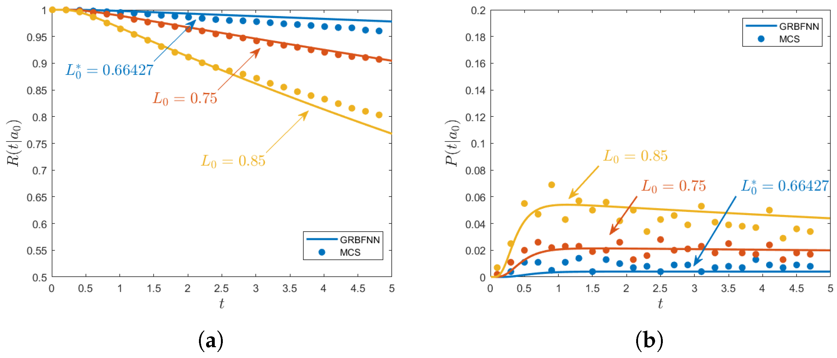
As can be clearly seen from Figure 9, under the optimal parameter $L_0^{*}=0.66427$ obtained by the PSO-GRBFNN algorithm, the system demonstrates high reliability. Moreover, as $L_0$ increases, the system reliability continuously decreases.

In the display of Figure 9, the solid line represents the solution results based on the GRBFNN algorithm, while the scattered points denote the solutions obtained through Monte Carlo Simulation (MCS). During the MCS process, we employ a large amount of random data to solve Equation (40) using the fourth-order Runge–Kutta method. Meanwhile, we take into account the boundary condition that the reliability function satisfies. Based on this, we conducted a statistical analysis on the simulation results and calculated the final outcomes accordingly. It is evident from the figure that the curves derived from the GRBFNN algorithm and MCS exhibit a high degree of fit, showing good consistency between the two. This phenomenon fully proves that the GRBFNN algorithm possesses high accuracy and reliability in solving such problems, effectively validating the algorithm’s effectiveness.

On the other hand, we conducted an in-depth analysis of the optimal parameter $L_0^{*}=0.66427$ obtained using the PSO-GRBFNN algorithm. From Figure 9a, it can be observed that the $L_0^{*}$ obtained through the algorithm proposed in this paper can indeed enable the system to achieve an optimal control state. Further observation reveals that over time, the system’s reliability value shows a continuous downward trend. However, when the selected time-delay parameter is not the optimal control parameter, the rate of decline in the reliability value significantly accelerates.

Figure 9b analyzes the situation from the perspective of the first-passage probability, which equally validates the superiority of the solved optimal control parameter $L_0^{*}$. When the system adopts non-optimal parameters, it exhibits the following variation pattern: in a relatively short time, the probability of the system experiencing a first passage is relatively high; as time progresses, the probability of first passage continuously decreases. This implies that the system faces a high risk of first passage in the short term, which may lead to a sharp decline in system performance or even failure. Conversely, when the solved optimal parameter $L_0^{*}$ is adopted, the system can better maintain a low first-passage probability, thereby ensuring better stability and reliability of the system.

Therefore, the above conclusions all indicate that the PSO-GRBFNN algorithm demonstrates significant effectiveness in finding optimal control parameters. That is, the algorithm can relatively accurately locate the parameters that optimize system performance, thereby effectively enhancing the overall reliability and stability of the system.

To further explore the degree of agreement between the results obtained by the GRBFNN algorithm and MCS, we conducted an error analysis of the system, and the specific analysis result is shown in

Table 1. Error between MCS and GRBFNN with respect to the reliability function. The numbers in red represent the minimum error and maximum error.

${\mathit{L}}_0^{*}=0.66427$			${\mathit{L}}_0=0.75$			${\mathit{L}}_0=0.85$
GRBFNN	MCS	Error	GRBFNN	MCS	Error	GRBFNN	MCS	Error
1.0000	0.9998	0.0002	0.9999	1.0000	0.0001	0.9997	0.9990	0.0007
0.9999	0.9988	0.0011	0.9989	0.9986	0.0003	0.9957	0.9926	0.0031
0.9996	0.9974	0.0022	0.9963	0.9946	0.0017	0.9876	0.9840	0.0036
0.9990	0.9962	0.0028	0.9926	0.9870	0.0056	0.9777	0.9728	0.0049
0.9984	0.9944	0.0040	0.9885	0.9820	0.0065	0.9672	0.9618	0.0054
0.9976	0.9926	0.0050	0.9842	0.9782	0.0060	0.9566	0.9510	0.0056
0.9968	0.9910	0.0058	0.9798	0.9742	0.0056	0.9460	0.9422	0.0038
0.9960	0.9890	0.0070	0.9755	0.9702	0.0053	0.9356	0.9316	0.0040
0.9952	0.9876	0.0076	0.9711	0.9648	0.0063	0.9252	0.9214	0.0038
0.9944	0.9858	0.0086	0.9667	0.9602	0.0065	0.9150	0.9082	0.0068
0.9936	0.9842	0.0094	0.9624	0.9560	0.0064	0.9048	0.9008	0.0040
0.9928	0.9828	0.0100	0.9581	0.9538	0.0043	0.8948	0.8922	0.0026
0.9920	0.9804	0.0116	0.9538	0.9506	0.0032	0.8849	0.8818	0.0031
0.9912	0.9784	0.0128	0.9495	0.9472	0.0023	0.8750	0.8722	0.0028
0.9903	0.9772	0.0131	0.9452	0.9422	0.0030	0.8653	0.8636	0.0017
0.9895	0.9766	0.0129	0.9410	0.9386	0.0024	0.8557	0.8542	0.0015
0.9887	0.9748	0.0139	0.9367	0.9346	0.0021	0.8462	0.8454	0.0008
0.9879	0.9740	0.0139	0.9325	0.9310	0.0015	0.8369	0.8376	0.0007
0.9871	0.9706	0.0165	0.9283	0.9282	0.0001	0.8276	0.8292	0.0016
0.9863	0.9684	0.0179	0.9242	0.9234	0.0008	0.8184	0.8226	0.0042
0.9855	0.9668	0.0187	0.9200	0.9192	0.0008	0.8093	0.8158	0.0065
0.9847	0.9648	0.0199	0.9159	0.9150	0.0009	0.8003	0.8100	0.0097
0.9839	0.9628	0.0211	0.9117	0.9118	0.0001	0.7915	0.8012	0.0097
0.9831	0.9616	0.0215	0.9076	0.9096	0.0020	0.7827	0.7958	0.0131
minimum error		0.0002	minimum error		0.0001	minimum error		0.0007
Maximum error		0.0215	Maximum error		0.0065	Maximum error		0.0131
Mean error		0.0107	Mean error		0.0107	Mean error		0.0031
Global mean error								0.0060

.

Regarding the error condition between the method proposed in this paper and MCS, we selected the three line segments displayed on Figure 9a as typical cases to analyze the results obtained from MCS and GRBFNN. After corresponding calculations, the data of the minimum error, maximum error, and average error were all listed in detail in Table 1.

It can be clearly seen from the data in the table that the overall average error is $0.0060$, the maximum error does not exceed $0.03$, and the minimum error is as low as the order of ${10}^{-3}$. This series of error data strongly indicates that the results obtained by GRBFNN are in high agreement with those from MCS, demonstrating relatively high accuracy and validity. This fully verifies the outstanding capability of GRBFNN in solving such problems.

In addition, we have also conducted an in-depth exploration of the impact of the initial amplitude $a_0$ on system reliability, covering its effects on the reliability function and the probability of the mean first-passage time. Relevant content can be found in Figure 10.

As can be clearly seen from Figure 10a, with the continuous increase in the initial amplitude, the reliability function exhibits a gradual downward trend. Moreover, when the initial amplitude gradually approaches the boundary of the safe region, this declining trend significantly accelerates. This implies that the larger the value of the initial amplitude $a_0$, the lower the system’s reliability will be, and the higher the probability of the system crossing the boundary for the first time, thereby making it more likely to cause structural damage or failure.

These research findings fully demonstrate that the magnitude of the initial amplitude has a significant influence on the likelihood of the system crossing the boundary. By observing Figure 10b, it can be found that when the initial amplitude $a_0=0.9$, the probability of the system crossing the boundary within a short period exceeds $50\%$, while the probability of crossing the boundary over a longer period is relatively low. Conversely, when the initial amplitude $a_0=0.5$, the probability of the system crossing the boundary within a short period is close to zero, and its probability of crossing the boundary in the long term remains relatively stable.

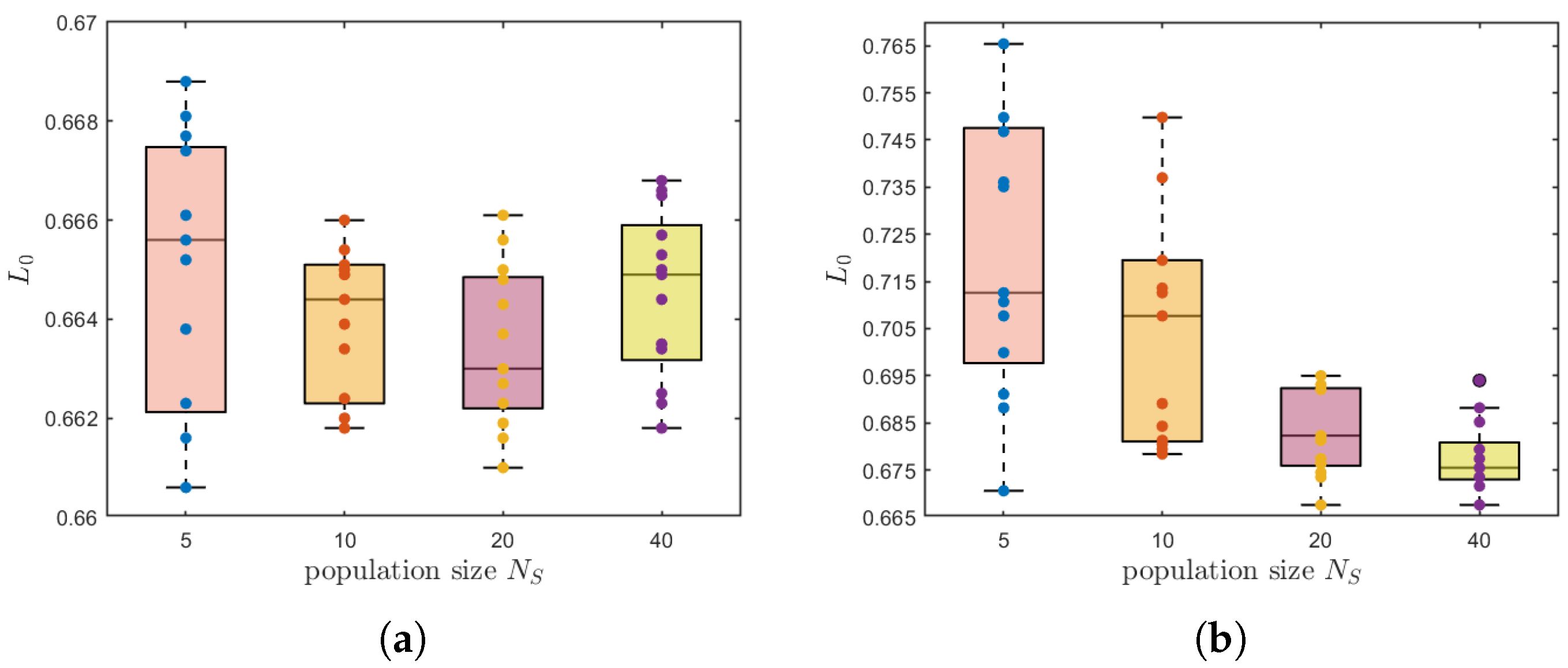
To more precisely and thoroughly evaluate the performance differences between the GA-GRBFNN and the PSO-GRBFNN, we carried out the following comparative analysis.

Through observation under the experimental conditions where the number of iterations $M_s=100$ and by changing the parameter of population size $N_s$, it is found in Figure 11 that PSO-GRBFNN can successfully obtain the optimal solution with a small population size. Moreover, as the population size increases, the fluctuation range of the obtained optimal solution is relatively small, demonstrating stable performance. In stark contrast, the optimal solution of GA-GRBFNN exhibits significant volatility, and the quality of the optimal solution obtained under these conditions shows a certain gap compared with that of PSO-GRBFNN.

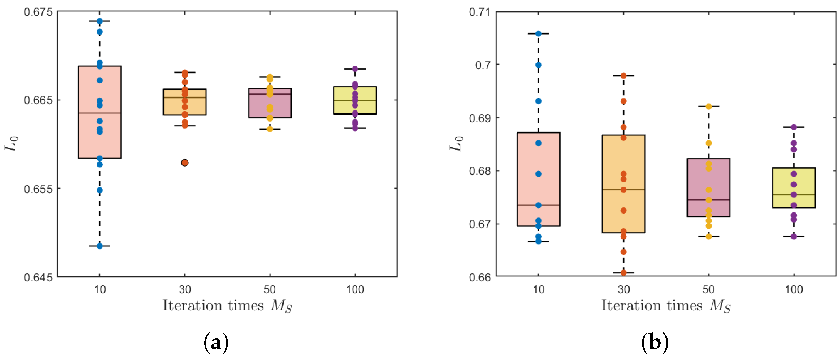
Through observation and analysis under the experimental setting, where the population size $N_s=40$ and by changing the parameter of population size $M_s$, it can be seen in Figure 12 that PSO-GRBFNN demonstrates outstanding performance: it can rapidly converge to the optimal solution within a relatively small number of iterations, and the errors between results obtained from different solving attempts are extremely minimal, indicating high stability. In contrast, GA-GRBFNN exhibits notably greater volatility during the solving process. However, as the number of iterations gradually increases, this degree of volatility shows a trend of gradual reduction. Nevertheless, even under the same conditions, the quality of the optimal solution obtained by GA-GRBFNN still falls short to a certain extent when compared with the results solved by PSO-GRBFNN.

From the comparative data on running time in Figure 13, it can be observed that under the experimental condition of a fixed number of iterations, the overall running time required by PSO-GRBFNN is consistently less than that of GA-GRBFNN. When the initial population size is fixed, the running times of the two are relatively close in scenarios with a small number of iterations. However, as the number of iterations continues to increase, the time consumed by GA-GRBFNN rises significantly. This phenomenon clearly indicates that, in terms of solving problems, PSO-GRBFNN possesses certain advantages over GA-GRBFNN in terms of operational efficiency.

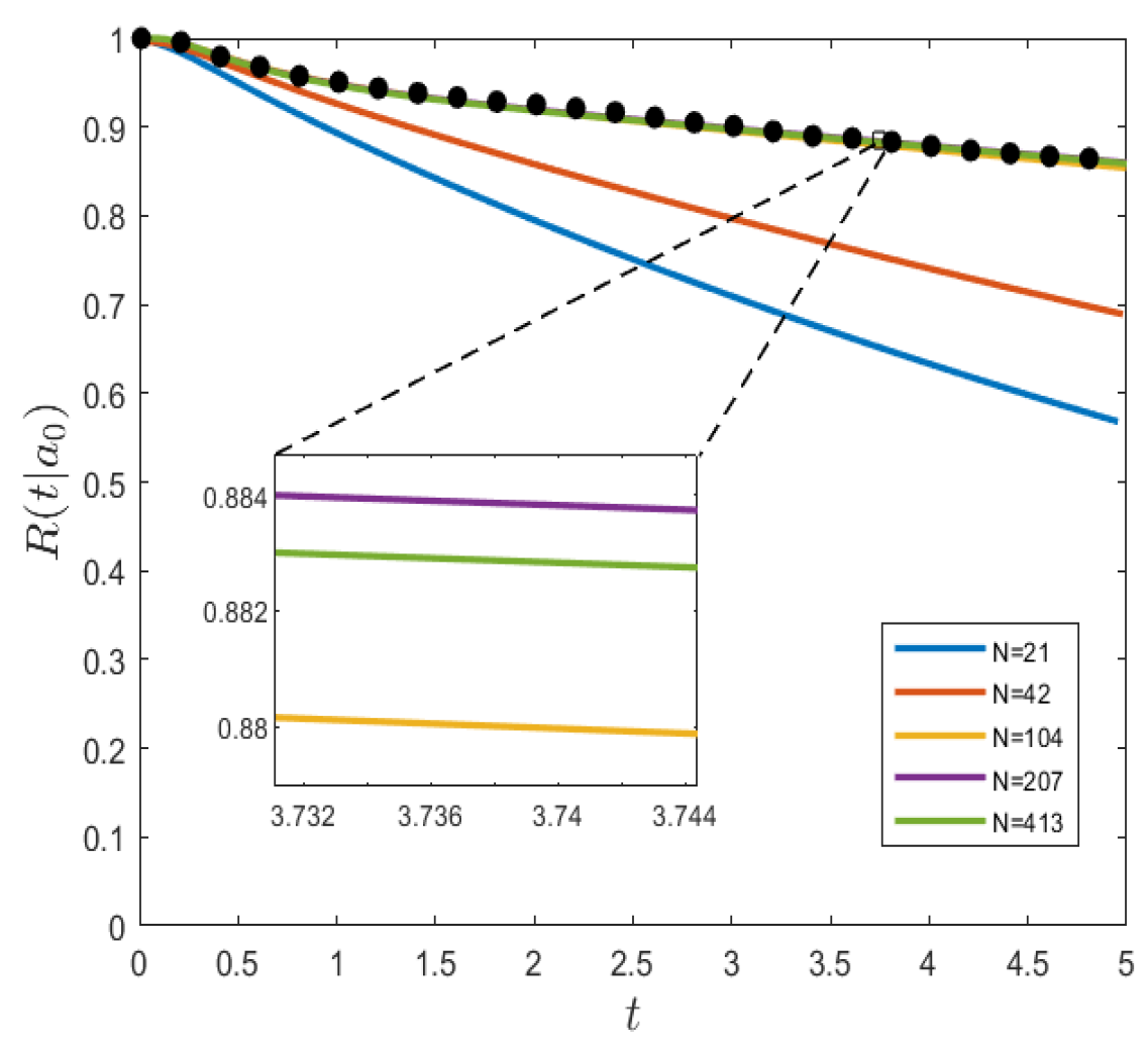
Finally, we conducted an analysis on the sensitivity of the number of neural network nodes to reliability. As shown in Figure 14, the lines in the graph represent the performance of the neural network in solving for reliability under different numbers of nodes, while the points represent the results obtained through MCS. It can be observed that when the neural network uses a relatively small number of nodes, its performance in solving for reliability is not satisfactory, and the errors are relatively large. However, when the number of nodes N in the neural network reaches or exceeds 104, the results obtained from the neural network are consistent with those from MCS. Moreover, as the number of neural network nodes further increases, the impact on the solution results becomes minimal.

6. Conclusions

The reliability optimization of NSD isolation systems with fractional-order damping under random excitation is a highly practical and meaningful topic. In this paper, a corresponding mathematical model is constructed for such systems, and the PSO-GRBFNN method is innovatively introduced to systematically investigate the impact of initial compression length on the optimal reliability of the NSD system.

Given the complexity of fractional-order damping, we successfully derive the BK equation satisfied by the reliability function using the generalized stochastic averaging method. On this basis, with the reliability function as the optimization objective and the BK equation along with its related constraints as limiting factors, an implicit optimization model is constructed. By leveraging the powerful solving and optimization capabilities of the PSO-GRBFNN algorithm, we obtain the optimal solution for the initial compression length. The study yields the following conclusions: the longer the compressed length of the system, the weaker its ability to control system reliability; when compressed to a certain length, the change in system reliability becomes no longer significant.

Secondly, by employing MCS to analyze the system reliability function and the mean first-passage probability, we fully demonstrate that the obtained time-delay control parameters can achieve optimal control of system reliability. Further comparison of the results obtained by the PSO-GRBFNN method with those from the previously proposed GA-GRBFNN method reveals that PSO-GRBFNN outperforms GA-GRBFNN in both solution effectiveness and efficiency. After an in-depth exploration of the relationship between algorithm performance and internal parameters, it is found that the number of neural nodes in the GRBFNN has a significant impact on the algorithm’s effectiveness. When the number of neural nodes reaches 104 or more, the algorithm performs even better.

This study provides a solid theoretical foundation for the reliability optimization of NSD isolation systems with fractional-order damping. Its core value lies in effectively enhancing the overall system reliability through optimization algorithms. The proposed PSO-GRBFNN method is not only applicable to the reliability optimization of coupled systems with controllers but also has broad applicability and can be applied to other similar reliability optimization and control problems in random dynamic systems. For example, in the aerospace field, aircraft are subject to random disturbances such as atmospheric turbulence. This method can be used to conduct in-depth analyses of the impact of these random disturbances on aircraft structures and related parameters, thereby improving aircraft safety and reliability. In wind power generation systems, reliability control methods can be employed to analyze the impact of random factors such as wind speed and direction on the system, optimize system design, and enhance system reliability and stability.

However, it must be pointed out that, like any modeling method, the method proposed in this study also has certain limitations. When dealing with high-dimensional parameter optimization or high-dimensional reliability research problems, one may face challenges such as a sharp increase in computational complexity and optimization difficulty. Therefore, in future research work, we will fully consider these limitations and actively explore more advanced solutions. Despite the aforementioned limitations, this study holds milestone significance in the field of non-explicit reliability optimization of random dynamic systems. Future research directions can focus on exploring other excellent hybrid optimization algorithms, such as the Simulated Annealing (SA) algorithm, as well as other machine learning techniques, to improve the efficiency and accuracy of solutions to optimization problems. At the same time, we will strengthen research on the universality of algorithms to enable them to adapt to a wider range of practical application requirements and provide more powerful technical support for the reliability optimization of random dynamic systems.