Fractional-Order Creep Hysteresis Modeling of Dielectric Elastomer Actuator and Its Implicit Inverse Adaptive Control

Abstract

Focusing on the dielectric elastomer actuator (DEA), this paper proposes a backstepping implicit inverse adaptive control scheme with creep direct inverse compensation. Firstly, a novel fractional-order creep Krasnoselskii–Pokrovskii (FCKP) model is established, which effectively captures hysteresis behavior and creep dynamic characteristics. Significantly, this study pioneers the incorporation of the fractional-order method into a hysteresis-coupled creep model. Secondly, based on the FCKP model, the creep direct inverse compensation is developed to combine with the backstepping implicit inverse adaptive control scheme, where the implicit inverse algorithm avoids the construction of the direct inverse model to mitigate hysteresis. Finally, the proposed control scheme was validated on the DEA system control experimental platform. Under both single-frequency and composite-frequency conditions, it achieved mean absolute errors of 0.0035 and 0.0111, and root mean square errors of 0.0044 and 0.0133, respectively, demonstrating superior tracking performance compared to other control schemes.

1. Introduction

Smart material actuators, including dielectric elastomer actuators and magnetostrictive actuators, are widely used in the aerospace industry, biomimetic robots, and smart healthcare due to their fast response speed, low energy consumption, and high micro displacement accuracy [1,2,3,4,5,6]. However, when the signal is input into the actuator, the hysteresis nonlinear relationship with multi-value, strong nonlinearity, and non-smoothness between the input and output arise, which can seriously damage the control effect and even cause the control system to diverge. Consequently, mitigating hysteresis nonlinearity in the motion control of smart material actuators remains a critical research challenge [7,8,9,10].

Many methods have been proposed to reduce the negative impact of hysteresis in the motion control of smart material actuators [11,12,13]. Currently, there are two main methods for dealing with hysteresis. The first is to design the closed-loop control scheme and rely on the robustness of the control algorithm to compensate for the errors caused by hysteresis in the control system [14,15]. This method has some effect on control systems with hysteresis input, but it does not directly deal with hysteresis; in the meanwhile, an over-reliance on robustness can increase the pressure of the control system. The second is to develop the direct inverse model of hysteresis as feed-forward compensation to offset the hysteresis [16] and then improve the control effect based on the feedback closed-loop control method. However, constructing a direct inverse model of hysteresis proves complex and difficult to implement widely, often leading to limited applicability. To address these challenges, ref. [17] first proposed the implicit inverse compensation method, and the principle is to design a search mechanism to iteratively optimize and extract the real control signal coupled in hysteresis, avoiding constructing a direct inverse hysteresis model and completing hysteresis compensation. This method has since garnered widespread acclaim from experts and scholars.

However, these existing hysteresis treatment approaches primarily apply to static hysteresis, whereas the hysteresis present in smart material actuators exhibits dynamic characteristics such as creep. Traditional hysteresis modeling typically focuses on constructing static hysteresis models, including the Jiles–Atherton model [18,19], Prandtl–Ishlinskii (PI) model [20,21], and Preisach model [22,23], which characterize the nonlinear hysteresis relationship to some extent but overlook the impact of creep characteristics. Creep refers to the time-dependent deformation of materials under external electric fields and mechanical stress [24], which manifests as gradual changes in the hysteresis relationship in smart material actuators. Numerous phenomenological models have been developed to characterize creep behavior, including logarithmic models [25], finite-dimensional linear time-invariant models [26], and the recently proposed creep operator model [27]. However, constructing these creep models relies on spring–damper physical frameworks, which involve numerous difficult-to-identify parameters, making it challenging to develop a universal adaptive control scheme capable of compensating for creep effects. Currently, methods for addressing creep are similar to those for hysteresis and can be broadly categorized into two approaches. The first relies on the robustness of the controller. For instance, ref. [28] modeled creep dynamics using a linear system and treated it as an uncertainty term during control. Ref. [29] proposed a model-driven robust control strategy for multi-degree-of-freedom soft robots, where the steady-state error induced by creep was mitigated using integral action in the outer control loop. However, robustness-based methods, while partially suppressing creep effects, exhibit limited performance. The second approach employs a feedforward compensator to counteract creep. Ref. [30] introduced a relative creep model and used a neural network for compensation, but the offline-trained network may suffer from compensation errors when input conditions vary. Ref. [31] utilized an LSTM network for feedforward creep compensation but relied on dynamic models rather than real experimental data during training, potentially introducing bias. Fractional-order creep models, leveraging the unique memory characteristics of fractional calculus, provide an efficient representation of creep behavior with fewer parameters and facilitate the design of direct inverse models. Ref. [32] implemented a fractional-order creep model and validated it in open-loop experiments, but their approach treated hysteresis and creep separately, neglecting their coupling effects. Ref. [33] combined hysteresis and creep in a unified fractional-order framework but ultimately simplified it to a linear relationship for control, potentially introducing errors. To date, research on modeling the coupled hysteresis-creep dynamics remains scarce, and the development of an inverse compensation scheme combined with adaptive control for effective dielectric elastomer actuator (DEA) control has yet to be explored.

DEA, composed of a VHB-4910 membrane and carbon conductive grease, often used as a flexible actuation unit for soft robots, operates based on the principle illustrated in Figure 1. Initially placed on a stationary frame with the elastomer membrane in a horizontal, non-conductive state, the DEA undergoes deformation under gravitational force when a load is applied, simulating its flexible actuation capability. Upon applying a driving voltage, the membrane experiences Maxwell force, viscoelastic force, and gravity, resulting in significant displacement and enabling DEA motion. The conical structure of the DEA is essential for its working principle and motion measurement, as it ensures uniform force distribution at the center when an electrostatic field is generated between the electrodes. This electrostatic force thins the dielectric elastomer membrane, causing in-plane expansion and deformation, with voltage variations adjusting the film thickness and motion. However, the DEA exhibits strong nonlinearities, such as complex hysteresis and creep, making precise control challenging.

In this paper, a backstepping implicit inverse adaptive control scheme based on creep direct inverse compensation for the motion control system of the DEA is proposed, and the effectiveness of the proposed control scheme is verified on the constructed dielectric elastomer drive motion platform. DEAs, as a core driver for soft biomimetic robots, benefit from precise control to support applications in the micro- and nano-manipulation of soft biomimetic robots. Notably, traditional approaches to addressing hysteresis in dielectric elastomer actuator motion control rely on static hysteresis models with limited consideration for creep characteristics. Therefore, a novel FCKP model has been proposed to describe the hysteresis and creep characteristics present in the motion control of DEA. Compared to other classical hysteresis models, the KP model uniquely incorporates a slope parameter, which enhances its ability to characterize diverse hysteresis behaviors. By combining fractional-order calculus with the KP model, the creep behavior is directly coupled into a more flexible KP framework. This approach avoids the issue of traditional series-connected models, which describe hysteresis and creep separately while neglecting their inherent coupling relationship. This study focuses on developing a hysteresis model that integrates creep effects and addresses this limitation. The primary contributions of this article are as follows:

• Innovatively integrates the fractional-order creep characteristics into the classical KP model, and the FCKP hysteresis model that can describe creep is first proposed. Compared with traditional description, this model enhances creep representation and simplifies parameter identification. To our best knowledge, no prior research has coupled fractional-order creep characteristics with the KP model to describe hysteresis phenomena, particularly in the modeling of dielectric elastomer actuators.
• A novel method combining direct creep inverse compensation and implicit inverse compensation is designed to eliminate the impact of creep-characteristic hysteresis on the control system. It is also found that the FCKP hysteresis model developed in this paper is more conducive to feed-forward compensation, thereby facilitating control scheme design.
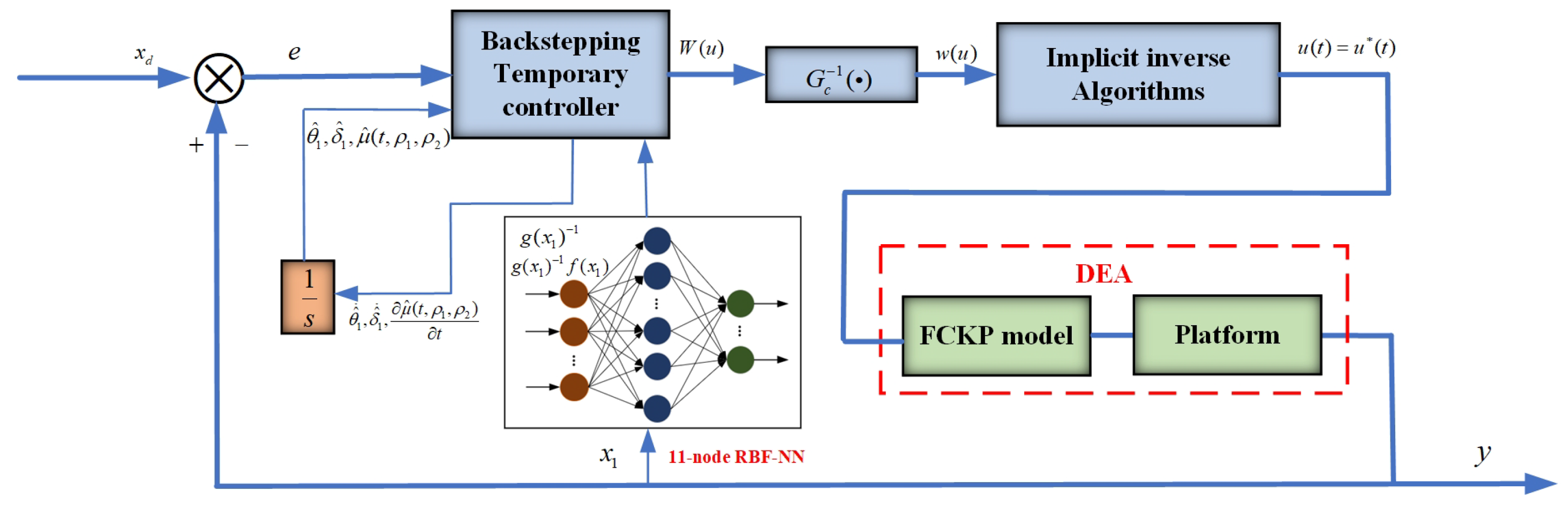
• An implicit inverse adaptive controller based on backstepping and direct creep inverse compensation is designed to control the DEA. Using a Radial Basis Function Neural Network (RBFNN) to estimate unknown nonlinear functions in a system, the control accuracy of the system is improved. The adaptive backstepping methods incorporating neural network approximation in [34,35,36] have achieved mature results. However, their control systems assume known gains for the control signals, unlike this study, where the gain is an unknown nonlinear function. Ref. [37] addresses unknown nonlinear gains but uses adaptive fuzzy control, which is less model-dependent. Since DEA requires high precision, a model-independent approach may degrade control performance. Finally, the effectiveness of this approach is validated on a self-built experimental platform.

The rest of this paper is as follows. Section 2 describes the relevant issues, constructs a model for DEAs, and designs an FCKP model to describe hysteresis phenomena with creep characteristics; Section 3 introduces the design of a backstepping implicit inverse adaptive controller based on creep direct inverse compensation; Section 4 conducted stability analysis on the designed control scheme; Section 5 describes the experimental platform for motion control based on dielectric elastomer actuation, verifying the effectiveness of the designed control scheme; Section 6 summarizes the practical significance of this research; Section 7 provides a conclusion of the study conducted in this paper.

2. System Descriptions and Preliminaries

2.1. Dielectric Elastomer Driven Dynamic Model

The dynamic model of the motion control system actuated by DEA can be expressed as [38]

$$\ddot{y}=g-{\displaystyle \frac{2\pi HR}{m}}(s_e-s_M+s_v)\sin \theta ,$$

(1)

where the viscoelastic stress $s_v={\displaystyle \sum _{i=1}^n}{\psi }_i({\lambda }_1\left(0\right)e^{{\displaystyle \frac{t}{{\varpi }_i}}}+{\int }_0^t{\dot{\lambda }}_1\left(s\right)e^{{\displaystyle \frac{s}{{\varpi }_i}}}ds)$, the electrical stress $s_M=\epsilon {\lambda }_{1,tot}{\lambda }_{2,tot}^2{\displaystyle \frac{W\left(u\right)}{H^2}}$, and the elastic stress $s_e={\upsilon }_e({\lambda }_{1,tot}-{\lambda }_{1,tot}^{-3}{\lambda }_{2,tot}^{-2})$ are calculated, respectively. During the material preparation process, the total stretching degree is represented by ${\lambda }_{i,tot}$, and the pre-stretching degree is represented by ${\lambda }_{pre}$. They satisfy the relationship ${\lambda }_{i,tot}={\lambda }_i{\lambda }_{i,pre}$, $i=1,2$ respresents the radial and circumferential direction for the membrane, respectively, and ${\lambda }_{1,pre}={\lambda }_{pre}={\lambda }_{2,tot}$. In addition, ${\lambda }_1={\displaystyle \frac{\sqrt{l_0^2+y^2}}{l_0}}$, and the deflection angle $\theta$ of the film satisfies $sin\theta ={\displaystyle \frac{y}{\sqrt{l_0^2+y^2}}}$. In terms of physical parameters, g is the gravitational acceleration, ${\upsilon }_e$ is the strain shear modulus, and $\epsilon$ is the dielectric constant of the film. ${\psi }_i$ and ${\varpi }_i$ ($i=1,2,\cdots ,n$) represent the spring stiffness and the damper damping coefficient, respectively. The initial thickness of the film is H, and the horizontal distance from a point to the center is denoted as R. The driving displacement of DEA is y, and the load mass is m. As the deflection angle of the film, $W\left(u\right)$ represents the hysteresis output displacement of the DEA with creep effect based on the input voltage $u\left(t\right)$.

Let $x_1=y$, $x_2={\dot{x}}_1$, considering the external disturbance, and (1) can be rewritten as [39]

$$\begin{array}{c}{\dot{x}}_1=x_2\hfill \\ {\dot{x}}_2=f\left(x_1\right)+g\left(x_1\right)W\left(u\right)+d\left(t\right)\hfill \\ y=x_1\hfill \end{array},$$

(2)

The system states are defined as $x_1$ (actuator displacement) and $x_2$ (velocity), which are governed by the electromechanical dynamics containing three fundamental components: $g\left(x_1\right)$ denotes an unknown continuous nonlinear mapping representing coupled electromechanical effects, $f\left(x_1\right)$ characterizes the hyperelastic response as a smooth unknown function, and $d\left(t\right)$ accounts for bounded external disturbances.

Table 1. Nomenclature table.

Symbol	Unit	Meaning
y	mm	The driving displacement of DEA
g	m/s2	The gravitational acceleration
$s_v$	N	The viscoelastic stress of DEA
$s_M$	N	The electrical stress of DEA
$s_e$	N	The elastic stress of DEA
H	mm	The initial thickness of the membrane
${\lambda }_{i,tot}$	/	The total stretching degree
${\lambda }_{i,pre}$	/	The pre-stretching degree
$\theta$	°	The deflection angle
${\upsilon }_e$	MPa	The strain shear modulus
$\epsilon$	F/m	The dielectric constant of the film
${\psi }_i$	N/m	The spring stiffness coefficient
${\varpi }_i$	N · s/m	The damper damping coefficient
R	mm	The horizontal distance from a point to the center
$W\left(u\right)$	mm	The hysteresis output displacement of the DEA with creep effect
${}_{t_0}{}^{GL}D_t^{\alpha }$	/	The fractional-order integral operator
$f(t-jh)$	/	The historical function value
${(-1)}^j\left(\begin{array}{c}\alpha \hfill \\ j\hfill \end{array}\right)$	/	The generalized binomial coefficient
$\Gamma$	/	The Gamma function
$\alpha$	/	The fractional order
$\kappa \left[u\right]\left(t\right)$	/	The output of the KP hysteresis model
$\mu \left({\rho }_1,{\rho }_2\right)$	/	The Gamma function
$R_0$	/	The two-dimensional integration region
${\kappa }_{\rho ,\delta }[u,{\xi }_{\rho ,\delta }]\left(t\right)$	/	KP kernel
${\rho }_1,{\rho }_2$	/	The KP kernel thresholds
${\phi }_R\left(\tau \right)$	/	The ridge function
$\delta$	/	The slope parameter of the KP kernel

shows some important symbols used in research. The following fundamental assumptions underpin the control design:

Assumption 1. 

External disturbances satisfy $\left|d\left(t\right)\right|\le \overline{d}$, $\forall t>0$, where $\overline{d}>0$ represents an unknown bounded constant.

Assumption 2. 

Reference trajectory $y_r$ and its derivatives ${[y_r,{\dot{y}}_r,{\ddot{y}}_r]}^T$ reside within a known compact set $\Omega \subset {\mathbb{R}}^3$ for all $t\ge 0$.

Assumption 3. 

Without losing generality, assume $g\left(x_1\right)>0$. Let $g_{min}\left(x_1\right)$ and $g_{max}\left(x_1\right)$ be positive constants such that $g_{min}\left(x_1\right)\le \left|g\left(x_1\right)\right|\le g_{max}\left(x_1\right)$. Furthermore, there exists a constant $\overline{g}\left(x_1\right)>0$ such that $\left|\dot{g}\left(x_1\right)\right|\le \overline{g}\left(x_1\right)$.

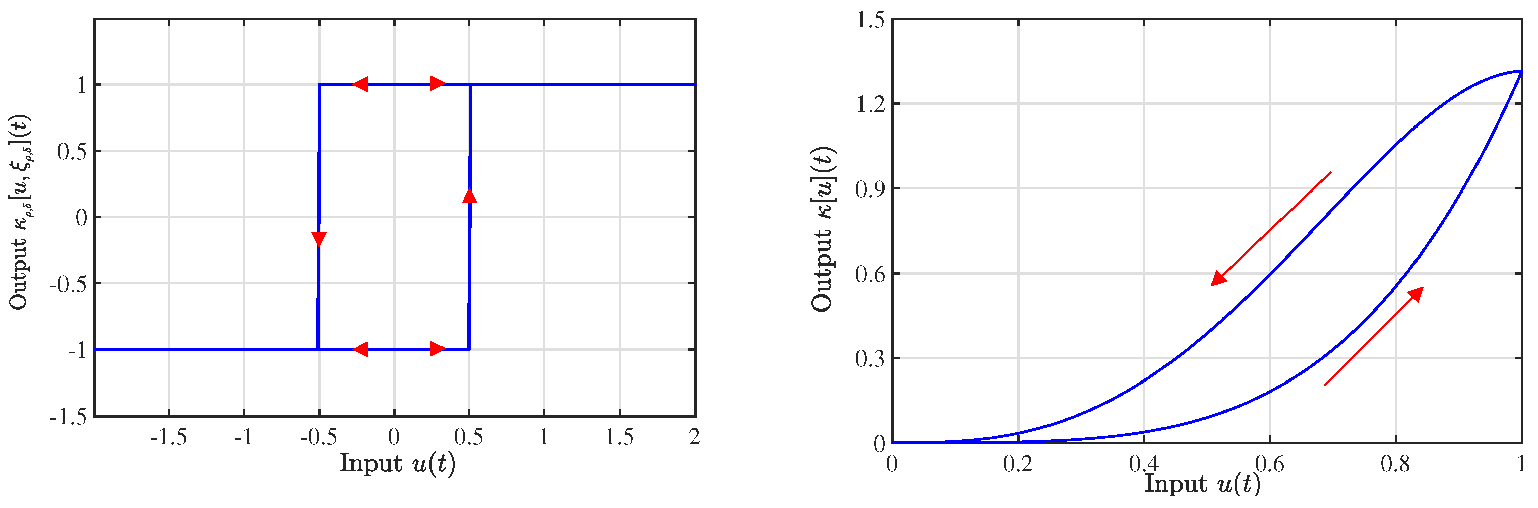
2.2. Modeling of Hysteresis with Creep

The DEA, known as a smart material actuator, inherently exhibit hysteresis nonlinearity. Traditional approaches typically use models like the PI or Preisach to capture the static characteristics of hysteresis. However, few models effectively describe the dynamic characteristics of hysteresis, such as creep behavior. Actually, previous studies have used fractional order to describe creep characteristics in hysteresis, such as concatenating the fractional order model $G\left(s\right)={\displaystyle \frac{1}{s^{\chi }}}$ with a hysteresis model based on differential equations to describe dynamic hysteresis in smart material actuators [40]. However, the existence of differential equations makes it too difficult to design effective control schemes. In this paper, the $Gr\ddot{u}nwald$–$Letnikov$ fractional-order integral operators are introduced to represent the hysteresis in DEA. $Gr\ddot{u}nwald$–$Letnikov$ fractional calculus is formulated as follows

$${}_{t_0}{}^{GL}D_t^{\alpha }f\left(t\right)=\underset{h\to 0}{lim}{h}^{-\alpha }\sum _{j=0}^N{(-1)}^j\left(\begin{array}{c}\alpha \hfill \\ j\hfill \end{array}\right)f(t-jh),$$

(3)

where ${}_{t_0}{}^{GL}D_t^{\alpha }$ defines the fractional-order integral operator, $t_0$ defines the limit of operation, h represents the step size, $f(t-jh)$ denotes the historical function value, and ${(-1)}^j\left(\begin{array}{c}\alpha \hfill \\ j\hfill \end{array}\right)$ represents the generalized binomial coefficient, which can be written as ${\displaystyle \frac{{(-1)}^j\Gamma (\alpha +1)}{\Gamma (j+1)\Gamma (\alpha -j+1)}}$, where $\Gamma$ is the Gamma function. $N=(t-t_0)/h$, $\alpha \in (-1,0)$ can be used to indicate the degree of creep.

The Krasnoselskii–Pokrovskii (KP) model is a widely utilized operator-based framework for modeling hysteresis loop [41,42,43]. It is constructed through the superposition of weighted KP kernels, which endows it with highly adaptable shape representation capabilities. The traditional KP model can describe the static hysteresis as follows

$$\kappa \left[u\right]\left(t\right)={\int \int }_{R_0}\mu ({\rho }_1,{\rho }_2){\kappa }_{\rho ,\delta }[u,{\xi }_{\rho ,\delta }]\left(t\right)d{\rho }_{1}d{\rho }_2,$$

(4)

where $\mu \left({\rho }_1,{\rho }_2\right)$ is the unknown density function, satisfying $\mu \left({\rho }_1,{\rho }_2\right)\ge 0$, $R_0$ is the two-dimensional integration region, ${\kappa }_{\rho ,and\delta }[u,{\xi }_{\rho ,\delta }]\left(t\right)$ represents KP kernel, which is defined as

$${\kappa }_{\rho ,\delta }[u,{\xi }_{\rho ,\delta }]\left(t\right)=\left\{\begin{array}{cc}\underset{\rho \in R_0}{max}\{{\phi }_R(u\left(t\right)-{\rho }_2),{\xi }_{\rho ,\delta }\left(t\right)\}\hfill & \dot{u}\ge 0\hfill \\ \underset{\rho \in R_0}{min}\{{\phi }_R(u\left(t\right)-{\rho }_1),{\xi }_{\rho ,\delta }\left(t\right)\}\hfill & \dot{u}<0\hfill \end{array}\right.,$$

(5)

where ${\rho }_1$ and ${\rho }_2$ represent the KP kernel thresholds, $u\left(t\right)$ is the input, and ${\phi }_R\left(\tau \right)$ is the ridge function defined as

$${\phi }_R\left(\tau \right)=\left\{\begin{array}{cc}-1,\hfill & \tau \le 0\hfill \\ -1+{\displaystyle \frac{2\tau }{\delta }},\hfill & 0<\tau <\delta \hfill \\ +1,\hfill & \delta \le \tau \hfill \end{array}\right.,$$

(6)

where $\delta >0$ represents the slope parameter of the KP kernel, and ${\xi }_{\rho ,\delta }\left(t\right)$ is defined as

$${\xi }_{\rho ,\delta }\left(0\right)={\kappa }_{\rho ,\delta }[u\left(t\right),{\xi }_0],$$

(7)

$${\xi }_{\rho ,\delta }\left(t\right)={\kappa }_{\rho ,\delta }[u\left(t\right),{\xi }_{\rho ,\delta }\left(t_i\right)],$$

(8)

where ${\xi }_0$ represents the initial value of the KP kernel. Figure 2(left,right) shows the KP kernel and its hysteresis loop, respectively, when ${\rho }_1=-0.5$, ${\rho }_2=0.5$, and $\delta$ = 0.01. It is important to note that the traditional KP model can only describe a static hysteresis relationship, adjusting the shape of the hysteresis loop by modifying the threshold and slope parameters. However, the hysteresis phenomenon in a smart material actuator is prone to creep, such as the DEA. Therefore, it is urgent to design a model to describe the hysteresis nonlinear relationship with the creep characteristics.

In this paper, a new fractional-order KP (FCKP) model will be introduced to describe the hysteresis with creep, which combines the fractional-order integration operator and the KP model. The FCKP model is defined as

$$\begin{array}{c}\hfill \begin{array}{cc}\hfill W\left[u\right]\left(t\right)& ={}_{t_0}{}^{GL}D_t^{\alpha }\kappa \left[u\right]\left(t\right)\hfill \\ \hfill & =\underset{h\to 0}{lim}{h}^{-\alpha }\sum _{j=0}^N{(-1)}^j\left({\displaystyle \genfrac{}{}{0pt}{}{\alpha }{j}}\right)\kappa \left[u\right](t-jh),\hfill \end{array}\end{array}$$

(9)

where $\kappa \left[u\right](t-jh)={\int \int }_{R_0}\mu \left({\rho }_1,{\rho }_2\right){\kappa }_{\rho ,\delta }\left[u,{\xi }_{\rho ,\delta }\right](t-jh)d{\rho }_{1}d{\rho }_2$, $u\left(t\right)$ is the input of the hysteresis, and $W\left[u\right]\left(t\right)$ is the output of the FCKP model. Usually, $t_0=0$ is used to describe hysteresis. In addition, some assumptions are necessary as follows.

Assumption 4. 

The DEA material exhibits a homogeneous microstructure with the degree of creep α remaining constant. Temperature fluctuations are assumed to have a negligible influence on α.

Assumption 5. 

Within a certain voltage range, the relative creep displacement of the DEA only depends on time t and ignores its relationship with the amplitude of input voltage.

Different hysteretic characteristics can be obtained by selecting different parameters $\delta ,\alpha$ in FCKP. Figure 3 and Figure 4 show the input–output relationship of the proposed FCKP model with $u\left(t\right)=0.5sin\left(2\pi t\right)$, $\mu ({\rho }_1,{\rho }_2)=0.004{\left[1+{\left({\displaystyle \frac{{\rho }_1-c}{c\sigma }}\right)}^2\right]}^{-1}{\left[1+{\left({\displaystyle \frac{{\rho }_2+c}{c\sigma }}\right)}^2\right]}^{-1}$. Let $c=2$, $\sigma =1$, $\alpha =0.05,t_0=0$; the different shapes of hysteresis can be obtained by selecting the different slope parameter $\delta$ in Figure 3; in the meanwhile, it can be clearly observed that the FCKP models can effectively describe the creep characteristics of hysteresis compared to a traditional KP model. Figure 4 illustrates the creep characteristics of the FCKP model with different $\alpha$, where $\alpha$ will affect the creep degree.

Remark 1. 

Unlike the physics-based modeling methods in [44,45], the proposed method in this work combines fractional-order dynamics with the KP model, and it not only accurately captures the coupled hysteresis–creep relationship but also facilitates the design of inverse compensators and seamless integration with adaptive control schemes. In contrast, while physics-based models can provide a more precise mechanistic description of hysteresis and viscoelasticity, their reliance on complex differential equations introduces significant challenges in controller design.

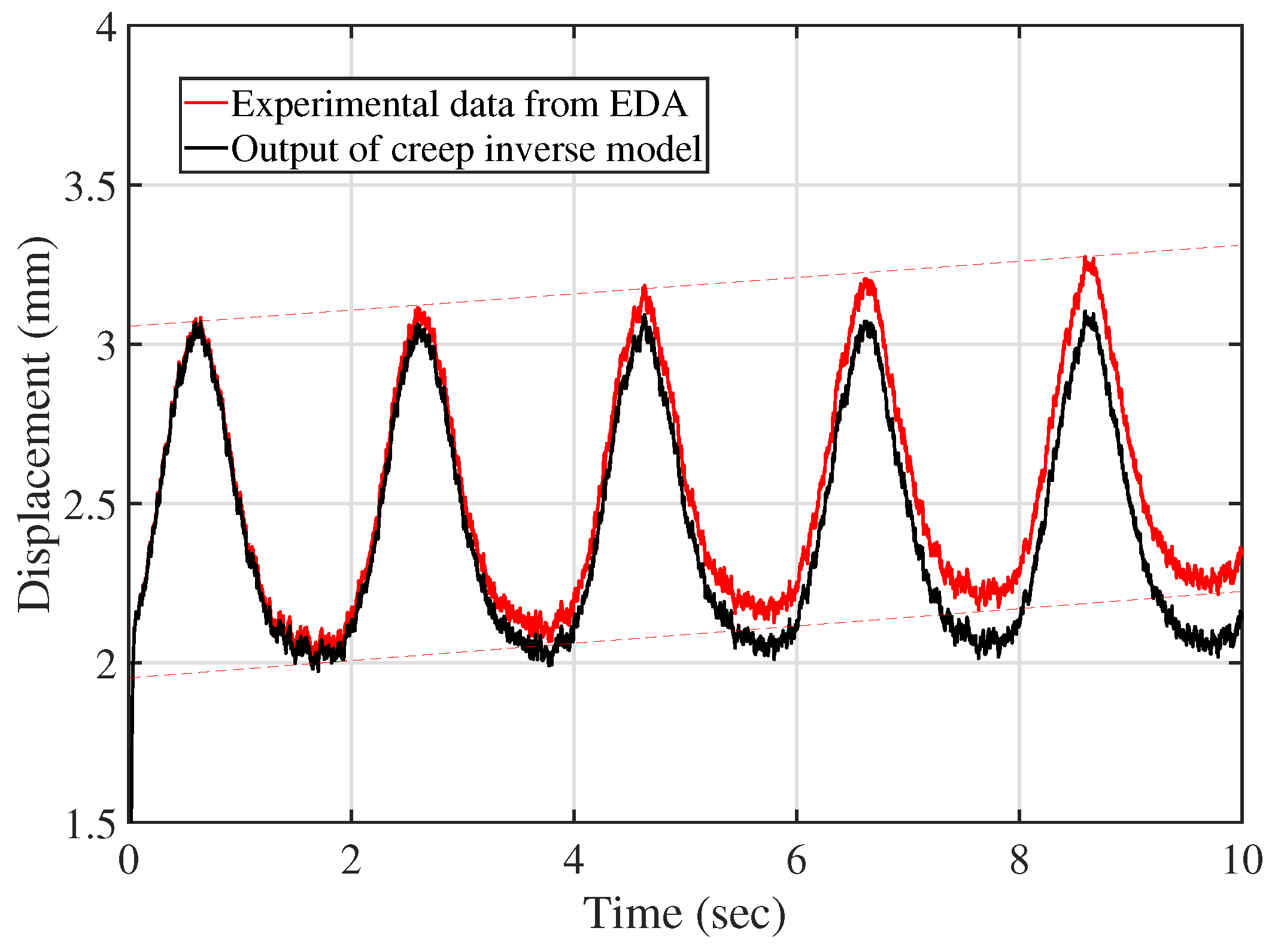
2.3. Creep Inverse Compensation

Considering the impact of creep on control performance, the inverse operation is designed to offset the creep in the FCKP model. It should be noted that the creep characteristics are described by using a fractional order, where the value of $\alpha$ determines the degree of creep. Therefore, the $-\alpha$-order fractional integral operation is employed to address the creep in the FCKP model. According to (9), the $-\alpha$-order integral operation is expressed as follows

$$\begin{array}{c}{}_{t_0}{}^{GL}D_t^{-\alpha }W\left(u\right)=\underset{h\to 0}{lim}{h}^{\alpha }{\displaystyle \sum _{k=0}^{N_k}}{(-1)}^k\left(\begin{array}{c}-\alpha \\ k\end{array}\right)\left\{\underset{h_1\to 0}{lim}{h}^{-\alpha }\right.\\ \left.{\displaystyle \sum _{j=0}^{N_j}}{(-1)}^j\left(\begin{array}{c}\alpha \\ j\end{array}\right)\kappa \left[u\right](t-jh-k{h}_1)\right\},\end{array}$$

(10)

where $N_k=t/h$, $N_j=(t-jh)/h_1$, and the quadratic coefficient satisfies

$$\sum _{j=0}^n\left(\begin{array}{c}\alpha \\ j\end{array}\right)\left(\begin{array}{c}\beta \\ n-j\end{array}\right)=\left(\begin{array}{c}\alpha +\beta \\ n\end{array}\right),$$

(11)

when $h\to 0$ and $h_1\to 0$, ${}_{t_0}{}^{GL}D_t^{-\alpha }W\left(u\right)=\kappa \left[u\right]\left(t\right)={\int \int }_{R_0}\mu \left({\rho }_1,{\rho }_2\right){\kappa }_{\rho ,\delta }\left[u,{\xi }_{\rho ,\delta }\right]\left(t\right)d{\rho }_{1}d{\rho }_2$ can ultimately be obtained. This also means that fractional-order inverse compensation can effectively offset the creep nonlinearity present in the hysteresis. Subsequently, compensation for the hysteresis nonlinearity can be carried out.

2.4. Function Approximation Using RBFNN

The proposed control scheme utilizes a Radial Basis Function Neural Network (RBFNN) to estimate system nonlinearity, leveraging their established approximation property for continuous functions on compact domains. Specifically, for any continuous function $F:\Omega \to \mathbb{R}$ defined on compact set $\Omega \subset {\mathbb{R}}^m$ ($m\in {\mathbb{N}}^{+}$), there exists a finite-dimensional parameterization with basis functions $\xi \left(x\right)=exp(-\parallel x-{\phi }_{i,k}{\parallel }^2/\left(2{\eta }_i^2\right))$ and optimal weight ${\theta }^{*}\in {\mathbb{R}}^p$ satisfying $\left|F\left(x\right)-{\theta }^{\ast T}\xi \left(x\right)\right|\le {\epsilon }_m,\forall x\in \Omega$, where ${ϵ}_m>0$ denotes the ultimate approximation bound. The function approximation residual $ϵ\stackrel{\Delta }{=}F\left(x\right)-{\theta }^{\ast T}\xi \left(x\right)$ is therefore bounded by $\left|ϵ\right|\le {ϵ}_m$. The optimal weight configuration is characterized by

$${\theta }^{*}=arg\underset{\theta \in {\mathbb{R}}^p}{min}\left(\underset{x\in \Omega }{sup}|Y\left(x\right)-F\left(x\right)|\right),$$

(12)

where $Y\left(x\right)$ denotes the RBFNN output signal.

3. Design of Control Scheme

3.1. Design of Hysteretic Temporary Controller

In this section, an adaptive backstepping method with a hysteresis implicit inverse compensator based on an RBFNN is introduced, where the creep in hysteresis is compensated in advance. The structural of the proposed control scheme is illustrated in Figure 5. Then, the controller is designed as follows:

Step 1: Define the tracking error as

$$e_1=x_1-x_d,$$

(13)

where $x_d$ represents the desired trajectory, while $x_1$ denotes the actual output of the DEA control system.

Define the Lyapunov function $V_1$ as follows

$$V_1={\displaystyle \frac{1}{2}}{e}_1^2,$$

(14)

and its derivative is

$${\dot{V}}_1=e_1{\dot{e}}_1=e_1(x_2-{\dot{x}}_d).$$

(15)

Choose the virtual controller as follows

$$x_{2d}=-k_1{e}_1+{\dot{x}}_d,$$

(16)

where $k_1$ is the positive design constant. Substituting (16) into (15), ${\dot{V}}_1=-k_1{e}_1^2\le 0$ holds. Therefore, $e_1$ is asymptotically stable.

Step 2: Define $e_2=x_2-x_{2d}$, and we have

$$\begin{array}{cc}\hfill {\dot{e}}_2& ={\dot{x}}_2-{\dot{x}}_{2d}\hfill \\ \hfill & =g\left(x_1\right)[g{\left(x_1\right)}^{-1}f\left(x_1\right)+W\left(u\right)-g{\left(x_1\right)}^{-1}{\dot{x}}_{2d}+{\displaystyle \frac{d}{g\left(x_1\right)}}].\hfill \end{array}$$

(17)

The RBFNN approximates the unknown continuous functions in (17) as follows

$$\begin{array}{cc}\hfill g{\left(x_1\right)}^{-1}f\left(x_1\right)& ={\theta }_1^{\ast T}{\xi }_1\left(x_1\right)+{\epsilon }_{11}\hfill \\ \hfill g{\left(x_1\right)}^{-1}& ={\delta }_1^{\ast T}{\eta }_1\left(x_1\right)+{\epsilon }_{12}.\hfill \end{array}$$

(18)

where ${\epsilon }_{11}$ and ${\epsilon }_{12}$ are the approximate errors, and ${\theta }_1^{\ast T}$, ${\delta }_1^{\ast T}$ and ${\xi }_1\left(x_1\right)$, ${\eta }_1\left(x_1\right)$ are the optimal weights and basic functions, respectively. Substituting (18) into (17), and one has

$${\dot{e}}_2=g\left(x_1\right)\{{\theta }_1^{\ast T}{\xi }_1\left(x_1\right)+{\epsilon }_{11}+W\left(u\right)-[{\delta }_1^{\ast T}{\eta }_1\left(x_1\right)+{\epsilon }_{12}]{\dot{x}}_{2d}+{\displaystyle \frac{d\left(t\right)}{g\left(x_1\right)}}\}.$$

(19)

The temporary control law is constructed as

$$W\left(u\right)=-{\widehat{\theta }}_1^T{\xi }_1\left(x_1\right)+{\widehat{\delta }}_1^T{\eta }_1\left(x_1\right){\dot{x}}_{2d}-k_2{e}_2,$$

(20)

where ${\widehat{\theta }}_1$ and ${\widehat{\delta }}_1$ are the estimated values of ${\theta }_1^{*}$ and ${\delta }_1^{*}$. Take (20) into (19), and we have

$${\dot{e}}_2=g\left(x_1\right)[{\tilde{\theta }}_1^T{\xi }_1\left(x_1\right)-{\tilde{\delta }}_1^T{\eta }_1\left(x_1\right){\dot{x}}_{2d}+D_1-k_2{e}_2],$$

(21)

where $k_2>0$ is the positive design constant, ${\tilde{\theta }}_1={\theta }_1^{*}-{\widehat{\theta }}_1$, ${\tilde{\delta }}_1={\delta }_1^{*}-{\widehat{\delta }}_1$, and throughout this paper, we define $\left(\widetilde{·}\right)=\left(·\right)-\left(\widehat{·}\right)$. A constant ${\epsilon }_1>0$ exists such that $\left|D_1\right|<{\epsilon }_1$, where $D_1$ is defined as

$$D_1={\epsilon }_{11}+{\epsilon }_{12}{\dot{x}}_{2d}+{\displaystyle \frac{d\left(t\right)}{g\left(x_1\right)}}.$$

(22)

Select the Lyapunov function $V_2$ as

$$V_2=V_1+{\displaystyle \frac{e_2^2}{2g\left(x_1\right)}}+{\displaystyle \frac{1}{2}}{\tilde{\theta }}_1^T{\Gamma }_{11}^{-1}{\tilde{\theta }}_1+{\displaystyle \frac{1}{2}}{\tilde{\delta }}_1^T{\Gamma }_{12}^{-1}{\tilde{\delta }}_1+{\displaystyle \frac{1}{2}}{\int \int }_{{\rho }_1\ge {\rho }_1}{\gamma }_{\mu }\tilde{\mu }{(t,{\rho }_1,{\rho }_2)}^{2}d{\rho }_{1}d{\rho }_2,$$

(23)

where ${\gamma }_{\mu }$ is a positive constant, and ${\Gamma }_{11}={\Gamma }_{11}^T>0$ and ${\Gamma }_{12}={\Gamma }_{12}^T>0$ are adaptive gain matrices. Then, the time derivative of $V_2$ is

$$\begin{array}{cc}\hfill {\dot{V}}_2& =-k_1{e}_1^2+e_2[W\left(u\right)-\widehat{W}\left(u\right)]+e_2[-k_2{e}_2+{\tilde{\theta }}_1^T{\xi }_1\left(x_1\right)-{\tilde{\delta }}_1^T{\eta }_1\left(x_1\right){\dot{x}}_{2d}+D_1]\hfill \\ \hfill & -{\displaystyle \frac{\dot{g}\left(x_1\right)}{2g{\left(x_1\right)}^2}}{e}_2^2-{\tilde{\theta }}_1^T{\Gamma }_{11}^{-1}{\dot{\widehat{\theta }}}_1-{\tilde{\delta }}_1^T{\Gamma }_{11}^{-1}{\dot{\widehat{\delta }}}_1+{\int \int }_{{\rho }_1\ge {\rho }_1}{\gamma }_{\mu }\tilde{\mu }(t,{\rho }_1,{\rho }_2){\displaystyle \frac{\partial \widehat{\mu }(t,{\rho }_1,{\rho }_2)}{\partial t}}d{\rho }_{1}d{\rho }_2,\hfill \end{array}$$

(24)

where ${\widehat{\theta }}_1$, ${\widehat{\delta }}_1$, $\widehat{\mu }(t,{\rho }_1,{\rho }_2)$ are updated by following

$$\begin{array}{cc}& {\dot{\widehat{\theta }}}_1={\Gamma }_{11}[e_2{\xi }_1\left(x_1\right)-{\sigma }_1{\widehat{\theta }}_1],\hfill \\ & {\dot{\widehat{\delta }}}_1={\Gamma }_{12}[-e_2{\eta }_1\left(x_1\right){\dot{x}}_{2d}-r_1{\widehat{\delta }}_1],\hfill \end{array}$$

(25)

$${\displaystyle \frac{\partial \widehat{\mu }(t,{\rho }_1,{\rho }_2)}{\partial t}}=-{\displaystyle \frac{K_{\rho ,\delta }[u,{\varsigma }_{\rho ,\delta }]\left(t\right)e_2}{{\gamma }_{\mu }}}+r_2\widehat{\mu }(t,{\rho }_1,{\rho }_2),$$

(26)

where ${\sigma }_1>0$, $r_1$, $r_2$ are positive constants.

Remark 2. 

It should be noted that (20) is designed as the temporary control law, while the actual control signal u is coupled in $W\left[u\right]\left(t\right)$, which means that extracting u from $W\left[u\right]\left(t\right)$ is a very important task. Due to the creep in hysteresis, before optimizing the actual control law by the implicit inverse algorithm, it is necessary to use a creep inverse compensator to counteract the influence of creep on control performance. That is, firstly, the degree of creep α can be identified through open-loop experiments using the least squares method and then using (10) to counteract the creep in hysteresis. At this time, the value of α is known, and $w\left[u\right]\left(t\right)$ can be obtained through creep inverse compensation. Finally, the implicit inverse algorithm is used to obtain the final control law u coupled in $w\left[u\right]\left(t\right)$.

3.2. Design of Implicit Inverse Algorithm for Hysteresis

After creep reverse compensation in hysteresis by (10), the actual control law is only coupled in $w\left[u\right]\left(t\right)={\int \int }_{{\rho }_1\ge {\rho }_2}\mu (t,{\rho }_1,{\rho }_2)K_{\rho ,\delta }[u,{\varsigma }_{\rho ,\delta }]\left(t\right)d{\rho }_{1}d{\rho }_2$. To proceed, use an implicit inverse algorithm to obtain the final control signal. Due to the density function $\mu (t,{\rho }_1,{\rho }_2)$ being unknown, its estimated value $\widehat{\mu }(t,{\rho }_1,{\rho }_2)$ is used to represent the temporary controller as

$$\begin{array}{c}\hfill {\int \int }_{{\rho }_1\ge {\rho }_1}\widehat{\mu }(t,{\rho }_1,{\rho }_2)K_{\rho ,\delta }[u,{\zeta }_{\rho ,\delta }]\left(t\right)d{\rho }_{1}d{\rho }_2=-{\widehat{\theta }}_1^T{\xi }_1\left(x_1\right)+{\widehat{\delta }}_1^T{\eta }_1\left(x_1\right){\dot{x}}_{2d}-k_2{e}_2,\end{array}$$

(27)

where $\widehat{\mu }(t,{\rho }_1,{\rho }_2)\ge 0$ is updated by (26).

Consider the actual input range of the hysteresis as $\left[u_{min},u_{max}\right]$. Without sacrificing generality, assume that $w\left[u\right]\left(t\right)$ corresponds to $u\left(t\right)$, where the input signal remains monotonic within the interval $t_i\le t\le t_{i+1}$. For each $t\in [t_i,t_{i+1}]$, the following condition holds

$$w\left[u_{min}\right]\left(t\right)\le {\int \int }_{{\rho }_1\ge {\rho }_1}\widehat{\mu }(t,{\rho }_1,{\rho }_2)K_{\rho ,\delta }[u,{\zeta }_{\rho ,\delta }]\left(t\right)d{\rho }_{1}d{\rho }_2\le w\left[u_{max}\right]\left(t\right).$$

(28)

Define variables $W_{\zeta }\left(t\right)$ and $u_{\zeta }\left(t\right)$, let $u_0\left(t\right)=u\left(t_i\right)$, and take $\zeta \in [0,u_{max}-u_{min}]$ to represent the optimal size; then,

$$u_{\zeta }\left(t\right)=u_0\left(t\right)+\zeta ,$$

(29)

$$W_{\zeta }\left(t\right)={\int \int }_{{\rho }_1\ge {\rho }_1}\widehat{\mu }(t,{\rho }_1,{\rho }_2)K_{\rho ,\delta }[u_{\zeta },{\varsigma }_{\rho ,\delta }]\left(t\right)d{\rho }_{1}d{\rho }_2.$$

(30)

The selection of $u^{*}\left(t\right)$ is determined as follows

If $w\left[u\right]\left(t\right)>w\left[u_{max}\right]\left(t\right)$, let $u^{*}\left(t\right)=u_{max}\left(t\right)$.

If $w\left[u\right]\left(t\right)<w\left[u_{min}\right]\left(t\right)$, let $u^{*}\left(t\right)=u_{min}\left(t\right)$.

If $w\left[u_{min}\right]\le w\left[u\right]\left(t\right)\le w\left[u_{max}\right]\left(t\right)$, the value of $u^{*}\left(t\right)$ can be obtained from the following steps.

Step 1: Increase $\zeta$ from 0.

Step 2: Calculate $u_{\zeta }\left(t\right)$ and $W_{\zeta }\left(t\right)$. If $W_{\zeta }\left(t\right)<w\left[u\right]\left(t\right)$, increase $\zeta$ continuously and go to Step 2; else, go to Step 3.

Step 3: Stop increasing $\zeta$ and record $\zeta$ as ${\zeta }_0$ at this time, and let $u^{*}\left(t\right)=u_{{\zeta }_0}\left(t\right)$.

Finally, based on the above algorithm, the actual control signal $u\left(t\right)$ can be obtained as

$$u\left(t\right)=u^{*}\left(t\right).$$

(31)

Remark 3. 

Since the controlled object contains unknown nonlinear functions, adaptive neural networks need to be employed to approximate $g{\left(x_1\right)}^{-1}f\left(x_1\right)$ and $g{\left(x_1\right)}^{-1}$, respectively, to facilitate the design of the controller. Due to the presence of not only creep but also hysteresis effects in the DEA, an implicit inverse compensator must be utilized to counteract the hysteresis and improve the control performance. It should be noted that neural network approximation introduces errors, and both these errors and the disturbance $d\left(t\right)$ have upper bounds. Therefore, through inequality-based scaling in the derivation process, the semi-negative definiteness of the Lyapunov function’s derivative is ensured, thereby guaranteeing system stability.

4. Stability Analysis

In this section, the stability of the proposed control scheme will be proved next. By using (25) and (26), the following can be obtained as

$$\begin{array}{cc}& {\dot{V}}_2=-k_1{e}_1^2-(k_2+{\displaystyle \frac{\dot{g}\left(x_1\right)}{2g{\left(x_1\right)}^2}})e_2^2+e_2{D}_1+{\sigma }_1{\tilde{\theta }}_1^T{\theta }_1\hfill \\ & +r_1{\tilde{\delta }}_1^T{\delta }_1+{\int \int }_{{\rho }_1\ge {\rho }_1}{r}_2\tilde{\mu }(t,{\rho }_1,{\rho }_2)\widehat{\mu }(t,{\rho }_1,{\rho }_2)d{\rho }_{1}d{\rho }_2.\hfill \end{array}$$

(32)

Let $k_2=k_{21}+k_{22}$ with $k_{21}$ and $k_{22}>0$. Then, (32) can be rewritten as

$$\begin{array}{cc}\hfill {\dot{V}}_2& =-k_1{e}_1^2-(k_{21}+{\displaystyle \frac{\dot{g}\left(x_1\right)}{2g{\left(x_1\right)}^2}})e_2^2+e_2{D}_1+{\sigma }_1{\tilde{\theta }}_1^T{\theta }_1+r_1{\tilde{\delta }}_1^T{\delta }_1\hfill \\ \hfill & -k_{22}{e}_2^2+{\int \int }_{{\rho }_1\ge {\rho }_1}{r}_2\tilde{\mu }(t,{\rho }_1,{\rho }_2)\widehat{\mu }(t,{\rho }_1,{\rho }_2)d{\rho }_{1}d{\rho }_2.\hfill \end{array}$$

(33)

Consider the following Young’s inequalities

$$\begin{array}{cc}\hfill & {\sigma }_1{\tilde{\theta }}_1^T{\theta }_1\le {\displaystyle \frac{{\sigma }_1{∥{\widehat{\theta }}_1∥}^2}{2}}-{\displaystyle \frac{{\sigma }_1{∥{\tilde{\theta }}_1∥}^2}{2}},\hfill \\ \hfill & r_1{\tilde{\delta }}_1^T{\delta }_1\le {\displaystyle \frac{r_1{∥{\widehat{\delta }}_1∥}^2}{2}}-{\displaystyle \frac{r_1{∥{\tilde{\delta }}_1∥}^2}{2}},\hfill \\ \hfill & {\int \int }_{{\rho }_1\ge {\rho }_1}{r}_2\tilde{\mu }(t,{\rho }_1,{\rho }_2)\widehat{\mu }(t,{\rho }_1,{\rho }_2)d{\rho }_{1}d{\rho }_2\le \hfill \\ \hfill & {\displaystyle \frac{r_2{\int \int }_{{\rho }_1\ge {\rho }_1}\widehat{\mu }{(t,{\rho }_1,{\rho }_2)}^2}{2}}-{\displaystyle \frac{r_2{\int \int }_{{\rho }_1\ge {\rho }_1}\tilde{\mu }{(t,{\rho }_1,{\rho }_2)}^2}{2}}\hfill \\ \hfill & -k_{22}{e}_2^2+e_2{D}_1\le {\displaystyle \frac{{\epsilon }_1^2}{4k_{22}}},\hfill \end{array}$$

(34)

one has

$$\begin{array}{cc}\hfill {\dot{V}}_2& \le -k_1{e}_1^2-(k_{21}+{\displaystyle \frac{\dot{g}\left(x_1\right)}{2g{\left(x_1\right)}^2}})e_2^2+[{\displaystyle \frac{{\epsilon }_1^2}{4k_{22}}}+{\displaystyle \frac{{\sigma }_1{∥{\widehat{\theta }}_1∥}^2}{2}}+{\displaystyle \frac{r_1{∥{\widehat{\delta }}_1∥}^2}{2}}\hfill \\ \hfill & +{\displaystyle \frac{r_2{\int \int }_{{\rho }_1\ge {\rho }_2}\widehat{\mu }{(t,{\rho }_1,{\rho }_2)}^2}{2}}]-[{\displaystyle \frac{{\sigma }_1{∥{\tilde{\theta }}_1∥}^2}{2}}+{\displaystyle \frac{r_1{∥{\tilde{\delta }}_1∥}^2}{2}}+{\displaystyle \frac{r_2{\int \int }_{{\rho }_1\ge {\rho }_2}\tilde{\mu }{(t,{\rho }_1,{\rho }_2)}^2}{2}}].\hfill \end{array}$$

(35)

Because $-(k_{21}+{\displaystyle \frac{\dot{g}\left(x_1\right)}{2g{\left(x_1\right)}^2}})e_2^2\le -(k_{21}-{\displaystyle \frac{\overline{g}\left(x_1\right)}{2g{\left(x_1\right)}^2}})e_2^2$, by choosing $k_{21}^{*}$ such that $k_{21}^{*}=k_{21}-{\displaystyle \frac{\overline{g}\left(x_1\right)}{2g{\left(x_1\right)}^2}}>0$, let $\varphi ={\displaystyle \frac{{\epsilon }_1^2}{4k_{22}}}+{\displaystyle \frac{{\sigma }_1{∥{\widehat{\theta }}_1∥}^2}{2}}+{\displaystyle \frac{r_1{∥{\widehat{\delta }}_1∥}^2}{2}}+{\displaystyle \frac{r_2{\int \int }_{{\rho }_1\ge {\rho }_2}\widehat{\mu }{(t,{\rho }_1,{\rho }_2)}^2}{2}}$. If we choose $k_1\ge {\displaystyle \frac{M}{2}}$, $k_{21}^{*}\ge {\displaystyle \frac{M}{2g\left(x_1\right)}}+{\displaystyle \frac{\overline{g}\left(x_1\right)}{2g{\left(x_1\right)}^2}}$, where M is a positive constant, and choose ${\sigma }_1,r_1,{\Gamma }_{11},\mathrm{and} {\Gamma }_{12}$ as suitable options that satisfy ${\sigma }_1\ge M{\lambda }_{max}\left\{{\Gamma }_{11}^{-1}\right\},r_1\ge M{\lambda }_{max}\left\{{\Gamma }_{12}^{-1}\right\}$, $r_2\ge M{\gamma }_{\mu }$, where ${\lambda }_{max}\left\{·\right\}$ is the largest eigenvalue of matrices, then we have

$$\begin{array}{cc}\hfill {\dot{V}}_2& \le -k_1{e}_1^2-k_{21}^{*}{e}_2^2+\varphi -[{\displaystyle \frac{{\sigma }_1{∥{\tilde{\theta }}_1∥}^2}{2}}+{\displaystyle \frac{r_1{∥{\tilde{\delta }}_1∥}^2}{2}}+{\displaystyle \frac{r_2{\int \int }_{{\rho }_1\ge {\rho }_2}\tilde{\mu }{(t,{\rho }_1,{\rho }_2)}^2}{2}}]\hfill \\ \hfill & \le -{\displaystyle \frac{M}{2}}{e}_1^2-{\displaystyle \frac{M}{2g\left(x_1\right)}}{e}_2^2-M[{\displaystyle \frac{1}{2}}{\tilde{\theta }}_1^T{\Gamma }_{11}^{-1}{\tilde{\theta }}_1\hfill \\ \hfill & +{\displaystyle \frac{1}{2}}{\tilde{\delta }}_1^T{\Gamma }_{12}^{-1}{\tilde{\delta }}_1+{\displaystyle \frac{1}{2}}{\int \int }_{{\rho }_1\ge {\rho }_2}{\gamma }_{\mu }\tilde{\mu }(t,{\rho }_1,{\rho }_2)d{\rho }_{1}d{\rho }_1]+\varphi \hfill \\ \hfill & \le -M{V}_2+\varphi .\hfill \end{array}$$

(36)

The stability and control performance of the closed-loop adaptive system are analyzed as follows. Assume that for all $t\ge 0$, there exist sufficiently large compact sets such that $e\in {\Omega }_1$, $\theta \in {\Omega }_{{\theta }_1}$, and $\delta \in {\Omega }_{{\delta }_1}$. Given bounded initial conditions, the following holds:

(1) All signals within the closed-loop system are bounded. From (36), we obtain

$${\dot{V}}_2\le -k_{\min }^{*}{∥e∥}^2+\varphi -{\displaystyle \frac{[{\sigma }_1{∥{\tilde{\theta }}_1∥}^2+r_1{∥{\tilde{\delta }}_1∥}^2+r_2{\int \int }_{{\rho }_1\ge {\rho }_1}\tilde{\mu }{(t,{\rho }_1,{\rho }_1)}^{2}d{\rho }_{1}d{\rho }_2]}{2}},$$

(37)

where $k_{min}^{*}$ is the minimum of $k_1$ and $k_{21}^{*}$. The error vector is defined as $e={\left[\begin{array}{cc}{e}_1& e_2\end{array}\right]}^T$. Consequently, the derivative of the global Lyapunov function remains negative as long as $e\notin \Omega =\{e\mid \parallel e\parallel >\sqrt{{\displaystyle \frac{\varphi }{k_{min}^{*}}}}\}$, or ${\tilde{\theta }}_1\notin {\Omega }_{\theta }=\left\{{\tilde{\theta }}_1\mid \parallel {\tilde{\theta }}_1\parallel >\sqrt{{\displaystyle \frac{2\varphi }{{\sigma }_1}}}\right\}$, or ${\tilde{\delta }}_1\notin {\Omega }_{\delta }=\left\{{\tilde{\delta }}_1\mid \parallel {\tilde{\delta }}_1\parallel >\sqrt{{\displaystyle \frac{2\varphi }{r_1}}}\right\}$, or $\tilde{\mu }(t,{\rho }_1,{\rho }_2)\notin {\Omega }_{\tilde{\mu }}=\left\{\tilde{\mu }(t,{\rho }_1,{\rho }_2)\mid \parallel \tilde{\mu }(t,{\rho }_1,{\rho }_2)\parallel >\sqrt{{\displaystyle \frac{2\varphi }{r_2}}}\right\}$. Applying the extended Lyapunov theorem, it follows that e, $\tilde{\theta }$, $\tilde{\delta }$, and $\tilde{\mu }(t,{\rho }_1,{\rho }_2)$ are uniformly ultimately bounded. Consider $e_1=x_1-x_{1d}$ and $x_{1d}$ are bounded; it follows that $x_1$ remains bounded. Similarly, since $e_2=x_2-x_{2d}$ and virtual controls $x_{2d}$ are bounded, the actual control law is also bounded. Moreover, as the system functions $f\left(x\right)$ and $g\left(x\right)$ are continuous, they remain bounded within any compact set. Thus, the optimal weights ${\theta }_1^{*}$ and ${\delta }_1^{*}$ are also bounded. Thus far, all signals in the closed-loop system are bounded.

(2) The output tracking error is reduced to a small neighborhood around zero with a proper selection of design parameters.

Let $\rho ={\displaystyle \frac{\varphi }{M}}>0$; then, (36) satisfies

$$0\le V_2\left(t\right)\le V_2\left(0\right)e^{-Mt}+\rho (1-e^{-Mt}).$$

(38)

Define $g_{max}=max\left\{1,g\left(x_1\right)\right\}$; then, one has

$$\begin{array}{cc}\hfill {\displaystyle \frac{1}{2g_{max}}}{e}_1^2+{\displaystyle \frac{1}{2g_{max}}}{e}_2^2& \le \rho +[V_2\left(0\right)-\rho ]e^{-Mt}<\rho +V_2\left(0\right)e^{-Mt}\hfill \\ \hfill e_1^2+e_2^2& <2g_{max}\rho +2g_{max}{V}_2\left(0\right)e^{-Mt}.\hfill \end{array}$$

(39)

Thus, for any $\lambda >\sqrt{2g_{max}\rho }$, there exists a constant T for all $t\ge T$, and the tracking error satisfies

$$\left|e_1\right|=\left|x_1\left(t\right)-x_d\left(t\right)\right|<\lambda ,$$

(40)

where $\lambda$ represents the size of a small residual set, which is determined by the approximation error and the controller parameters $k_{21},{\sigma }_1,r_1,r_2$, as well as the adaptive gains ${\Gamma }_{11},{\Gamma }_{12}$. It is evident that increasing the control gain $k_i$, adaptive gain ${\Gamma }_i$, and the number of neural network nodes enhances tracking performance.

Remark 4. 

The rules of the selections of the design parameters could refer to the following steps. Firstly, the value of the optimization step size ζ in an implicit inverse algorithm should be chosen as 0.01 to guarantee control performance. Secondly, according to the above procedures, (35) and (36), the design parameters ${\sigma }_1,r_1,and r_2$ could be chosen. Thirdly, concerning the range of $k_1$ and $k_2$ in (35), the design parameters could be chosen. Then, all of the design parameters in the control system could be set.

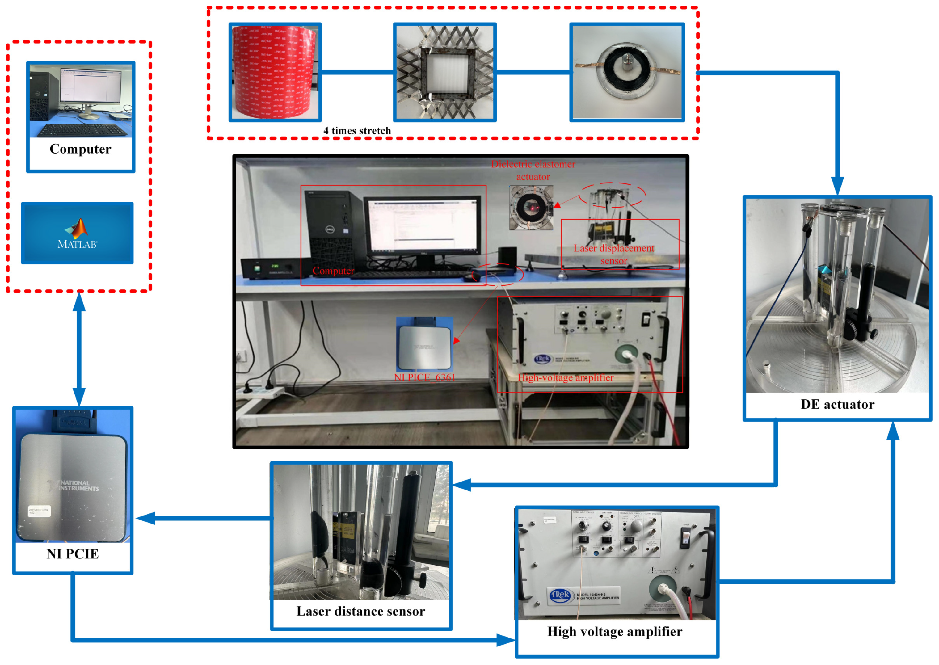
5. Experimental Verification

In this paper, the experimental platform depicted in Figure 6 is employed to validate the proposed DEA control scheme, which includes the following components:

• Preparation of DEA: Select a dielectric elastomer membrane based on VHB-4910 (Minnesota Mining and Manufacturing, St. Paul, MN, USA) material; fix the pre-stretched film on a polymethylmethacrylate ring; the DEA has an inner diameter of 40 mm and an outer diameter of 60 mm. Carbon conductive grease 864-80G (M.G. Chemicals, Burlington, ON, Canada) is uniformly applied to the annular areas on both sides of the DEA. Then, 20 g load mass is positioned at the center of the DEA membrane.
• The LK-H152 laser displacement sensor (Keyence, Osaka, Japan) measures the loaded weight’s displacement in the DEA experiment with a ±40 mm range and a 10 µs sampling period.
• The PCIe-6361 (National Instruments, Austin, TX, USA) multi-functional I/O device handles data transmission and analog-to-digital conversion in the DEA experiment. It supports various I/O channels, sampling rates, and output rates with a maximum single-channel sampling rate of 2.00 M/s and an input/output range of ±10 V.
• The TERK10/40A-HS voltage amplifier (TREK, Inc., Lockport, NY, USA) amplifies the PCIe-6361 voltage signal with a fixed gain of 1000 V/V.
• The computer (Dell, Round Rock, TX, USA) with Intel i7-9700 CPU (3.00 GHz) is used to generate control signals by executing the control algorithm to drive the DEA to achieve tracking control and perform experimental data processing.

In this experimental platform, the control signal designed in MATLAB R2022a is transmitted from the computer to a PCIe-6361 NI data acquisition board, where it is converted from digital to analog. The analog signal is then amplified by a TERK10/40A-HS high-voltage amplifier before being applied to the dielectric elastomer actuator. A LK-H152 laser displacement sensor measures the membrane displacement in real time, and the feedback data are sent back to the computer, completing the closed-loop control system.

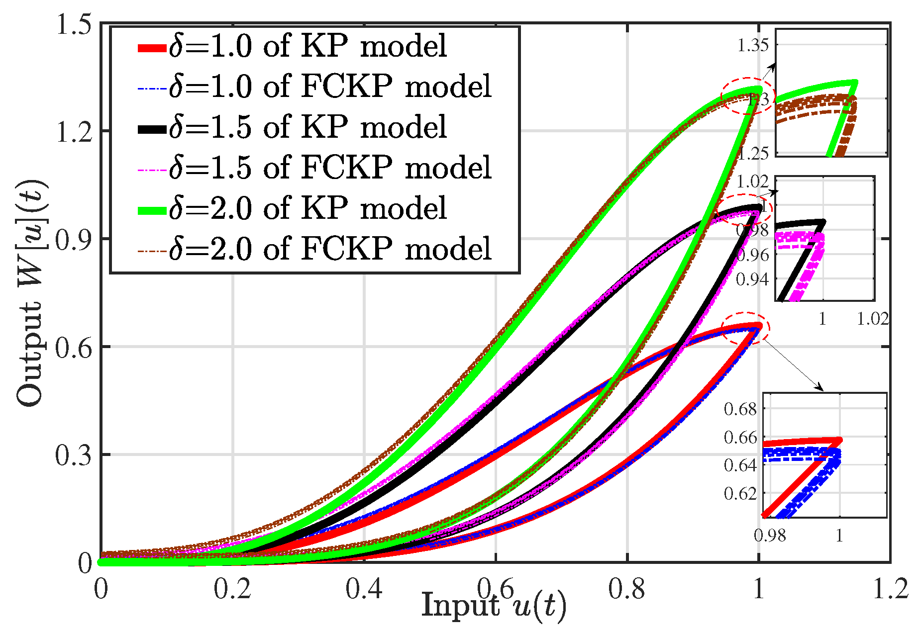
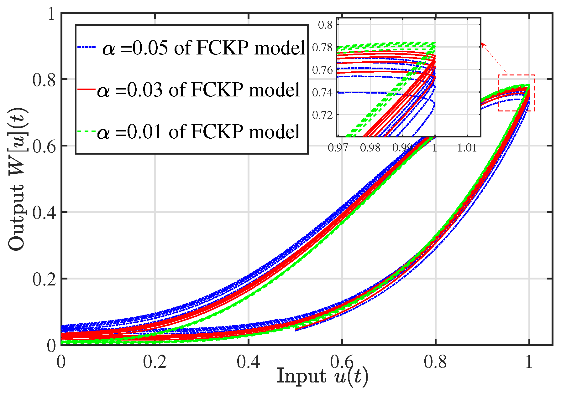
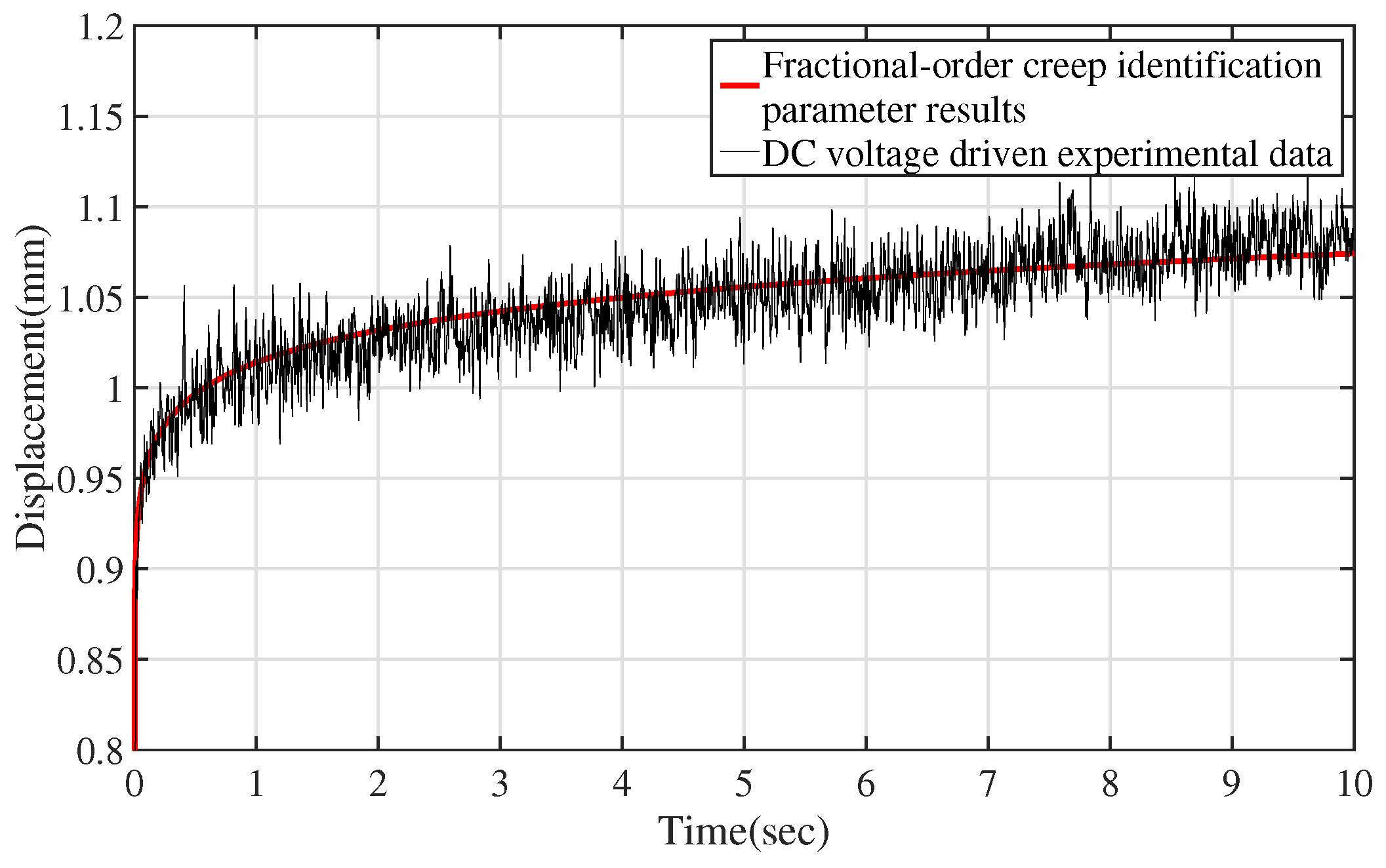
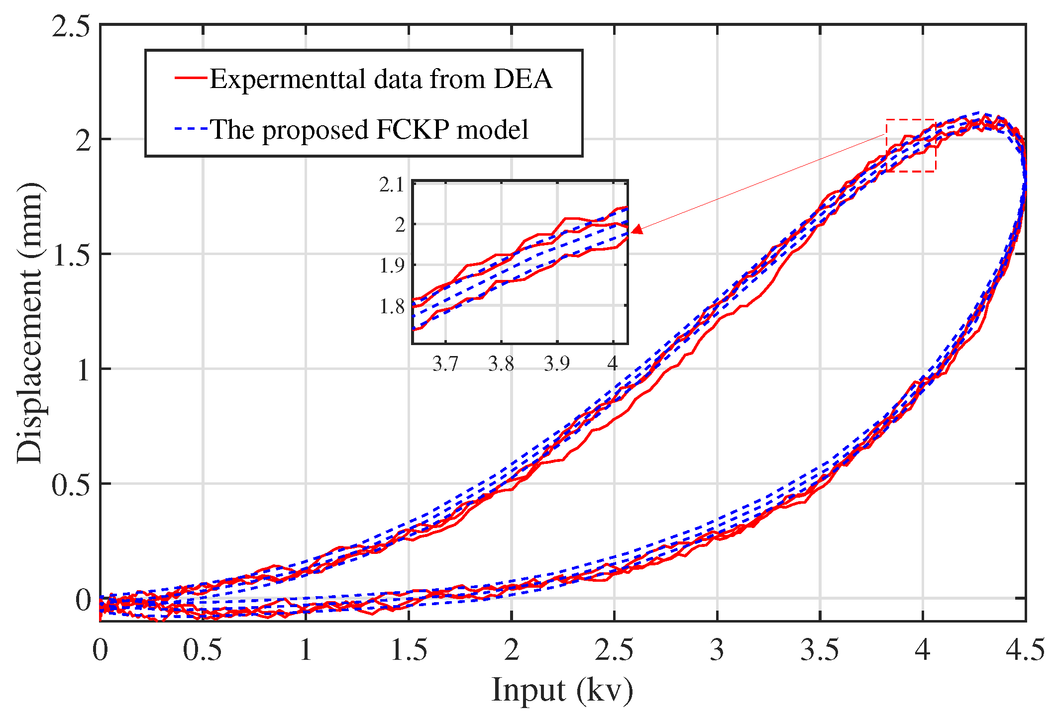
5.1. Experimental Validation of FCKP Model

Parameters $\delta$ and $\alpha$ need to be designed to more accurately describe the hysteresis nonlinear relationship, and two sets of experiments are conducted on the DEA experimental platform. The first one makes the input voltage a fixed value. Under constant input, the output of the hysteresis model is also a constant, but the output with creep is not a constant and has a certain upward trend, which is caused by the creep effect. Therefore, to obtain the value of the creep degree coefficient $\alpha$, we conducted an open-loop experiment with the input $u_k=2.25$ kV before the control experiments to avoid the influence of hysteresis on the identification of $\alpha$. Subsequently, using the least squares method in conjunction with (9), we successfully identified $\alpha =0.02$. By comparing the experimental data with the model output, as shown in Figure 7, it can be observed that the creep effect of the established model exhibits strong consistency with the actual creep behavior. The other set of experiments is used to let the input $u_d=2.25sin\left(10\pi t\right)+2.25$ (kV) and select an appropriate density function, $\delta$, and the identified $\alpha$. The experimental results are shown in Figure 8, from which it can be seen that the designed FCKP model has good performance in describing the hysteresis nonlinearity with creep in the DEA. Figure 9 shows the output after using creep inverse feedforward compensation, and it can be clearly seen that the creep effect in the DEA has been improved.

Remark 5. 

It should be noted that α represents the degree of creep, and a larger value indicates more pronounced time-varying displacement characteristics induced by creep. During its identification, open-loop experiments and the least squares method may also reduce model accuracy, while unknown disturbances in the environment may affect the identification results of α. Therefore, during the experiment, the test bench was placed in an enclosed experimental space to minimize the influence of airflow, and environmental temperature and vibration isolation were strictly monitored. Finally, multiple repeated experiments were conducted to average the results and reduce random errors in the identification.

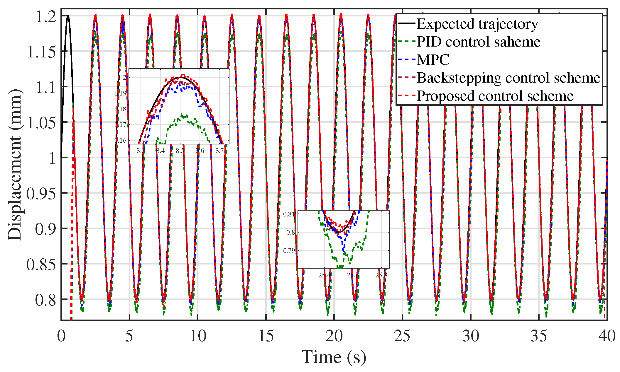
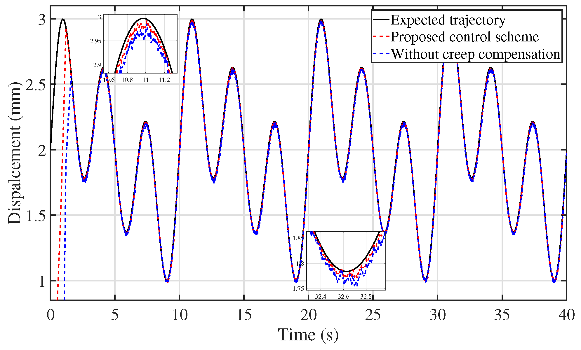
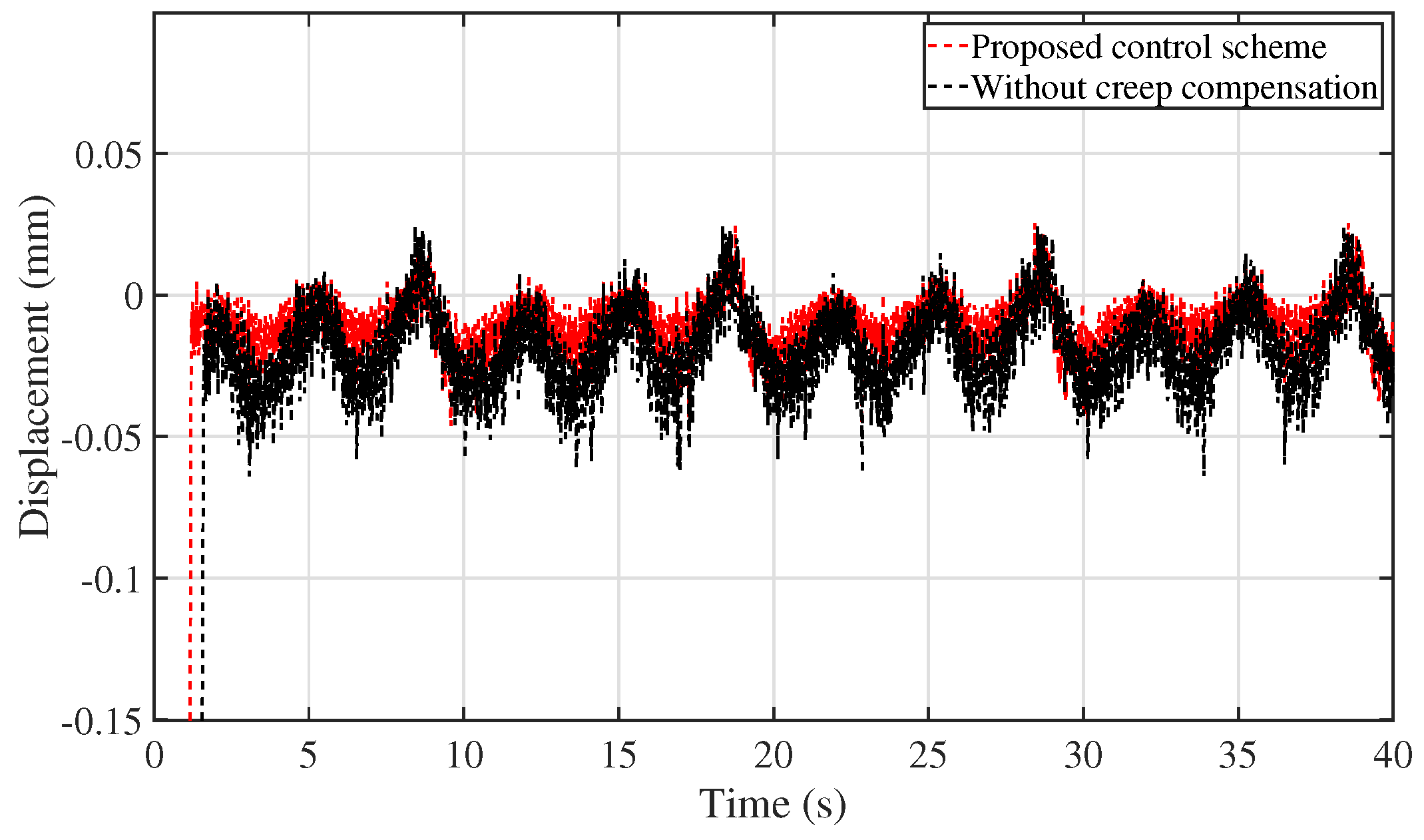
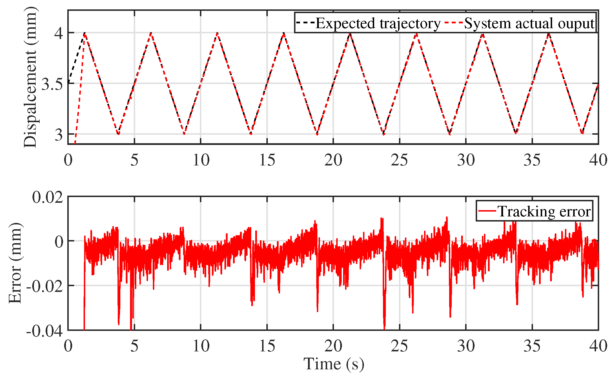
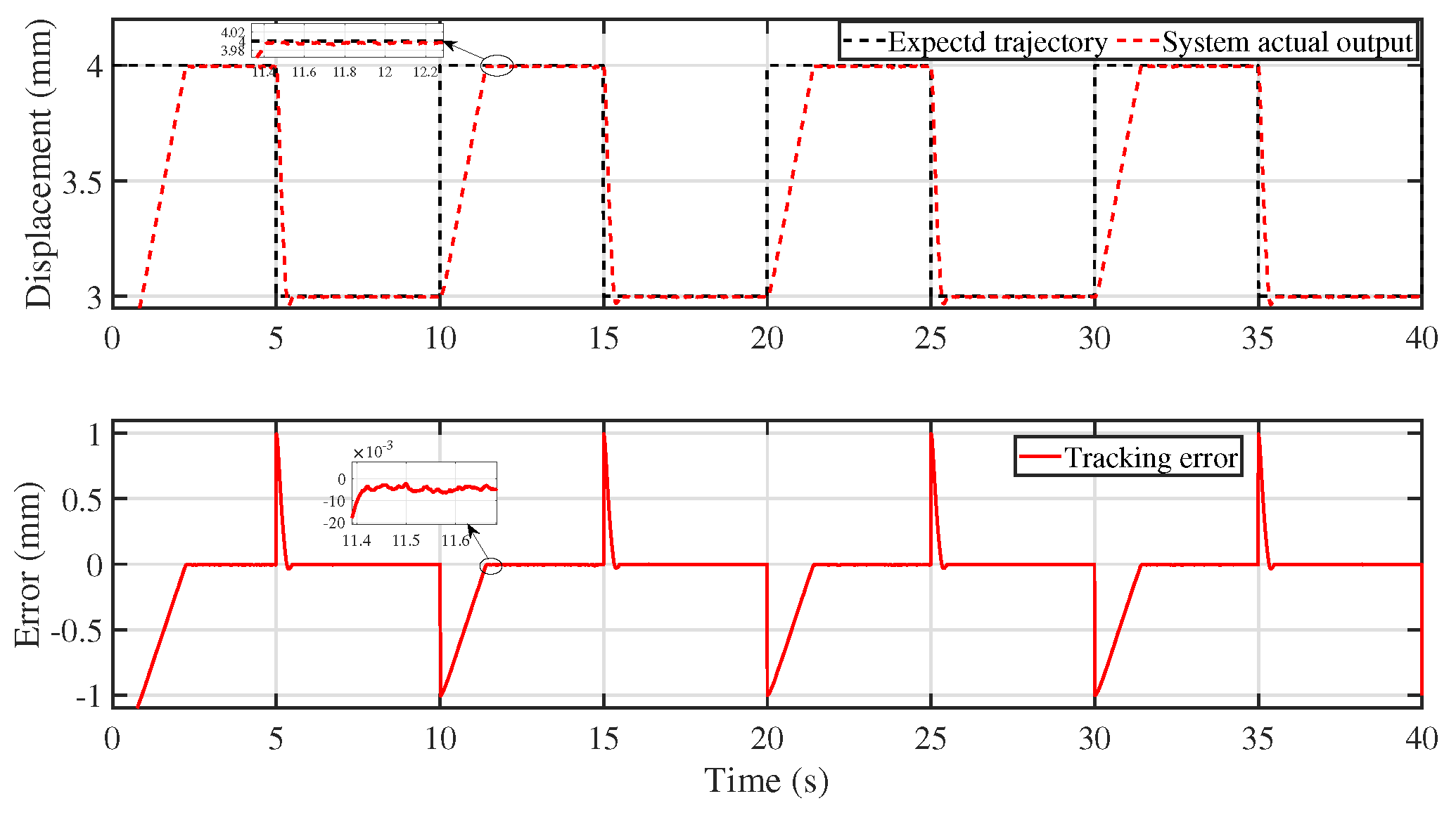
5.2. Experimental Validation of Control Performance

To validate the proposed control scheme, closed-loop tracking experiments are conducted on the DEA platform using single-frequency and compound-frequency reference trajectories. The control performance of the proposed scheme is compared with backstepping control without hysteresis, the model predictive control scheme, and classical PID control. Note that for nonlinear system control, existing algorithms need iterative parameter tuning to optimize performance. The experimental results of the four control algorithms were obtained after multiple tests, using the best-performing parameter set for comparison. In the experiments, the design parameters for the proposed control scheme are set as follows: $k_1=k_2=3.5$, ${\Gamma }_{11}={\Gamma }_{12}=diag\left\{2\right\}$, ${\sigma }_1=r_1=0.2$, $r_2=10$, and ${\gamma }_{\mu }=0.1$, and the initial values of estimations are selected as ${\widehat{\theta }}_1\left(0\right)={\widehat{\delta }}_1\left(0\right)=0$ and $\widehat{\mu }(0,{\rho }_1,{\rho }_2)=0.01$, the centers of basis functions in RBFNN are evenly spaced in [−1, 1] with 11 nodes, where ${\eta }_i=1,i=1,\dots ,11$. For the implict inverse algorithm, select $\zeta =0.01$. The sampling time of the MPC controller is 0.01 s, the experimental time is 40 s, the predictive horizon is 15, and the control horizon is 5. Consider that the maximum input of the high-voltage amplifier is 10 V, and the input constraint is [0, 10]. The input weight and rate weight are 0 and 0.75, respectively, and the output weight is 0.13. Setting the PID parameter, $K_P=0.8,K_I=1.67$ and $K_D=0.01$.

Due to the DEA being the flexible smart material, its working process is usually at low frequencies, the expected trajectory is chosen as $x_{d1}\left(t\right)=0.2sin\left(\pi t\right)+1.0$, and the experimental results are shown in Figure 10, Figure 11, Figure 12, Figure 13 and Figure 14. Figure 10 and Figure 11 show the comparisons of tracking performances and tracking errors, respectively. The results demonstrate that the proposed control scheme achieves the best control performance. The error accuracy of different control methods is summarized in

Table 2. Single-frequency tracking errors accuracy.

Kind of Tracking Error	MAE	RMSE
Proposed control scheme	0.35 × 10−2	0.44 × 10−2
Backstepping control	0.46 × 10−2	0.71 × 10−2
PID control	2.55 × 10−2	3.04 × 10−2
MPC	0.58 × 10−2	0.8 × 10−2

. The mean absolute error (MAE) is defined as $MAE={\sum }_{k=0}^N\left|e_1\left(k\right)\right|/N$, and the root mean square error (RMSE) is given by $RMSE=\sqrt{{\sum }_{k=0}^N{e}_1^2\left(k\right)/N}$, where $N=\mathrm{400,000}$. It obvious that compared to traditional backstepping control, the MPC scheme, and PID control methods, the proposed control scheme achieves smaller tracking errors with all parameters optimized. The control scheme proposed in this paper only employs the fractional-order method to describe and compensate for creep behavior. Compared to purely fractional-order modeling and control methods, it imposes a much smaller computational burden. On the other hand, learning-based control methods heavily rely on data and may produce significant errors when dealing with untrained operating conditions. Therefore, such methods are not suitable for real-time control applications requiring fast response. Figure 12 presents the estimation trajectories of $∥{\widehat{\theta }}_1∥,∥{\widehat{\delta }}_1∥$ with $∥{\widehat{\theta }}_1∥,∥{\widehat{\delta }}_1∥$ being the norm of ${\widehat{\theta }}_1,{\widehat{\delta }}_1$, and Figure 13 shows the 3D trajectory of $\widehat{\mu }(t,{\rho }_1,{\rho }_2)$. Figure 14 shows the control signal of the proposed scheme.

To verify the effectiveness of the developed control scheme, a multi-frequency composite trajectory $x_{d1}\left(t\right)=0.2sin\left(0.4\pi t\right)+0.4sin\left(0.2\pi t\right)+0.6sin\left(0.6\pi t\right)+2$ was adopted for comparison with a backstepping-based implicit inverse control scheme without creep inverse compensation. Figure 15 and Figure 16 show the tracking performance and tracking error, where all control parameters are the same as those in the above experiment. The experimental results confirm that the proposed control scheme achieves the best performance. The quantitative error accuracy is presented in

Table 3. Composite-frequency tracking error accuracy.

Kind of Tracking Error	MAE	RMSE
Proposed control scheme	0.0111	0.0133
Without creep compensation	0.0202	0.0235

.

Additionally, to further validate the effectiveness of the proposed control scheme, identical design parameters were maintained as in the previous experiment. Experimental tests were conducted using triangular and square waves as desired trajectories with results shown in Figure 17 and Figure 18. As observed from Figure 17 and Figure 18, although triangular and square waves are non-smooth functions, the proposed control scheme still achieved favorable tracking performance.

6. Practical Implications

The practical significance of this research lies in significantly improving the control accuracy of the DEA. By constructing a novel FCKP model, it effectively addressed the modeling challenges of hysteresis and creep dynamic characteristics while combining direct creep inverse compensation with implicit inverse compensation methods to enhance the DEA control performance. DEAs are widely used as flexible drive units in soft biomimetic robots, which are increasingly being developed for miniaturization and micro/nano-scale operations, making improved control accuracy particularly important. Currently, research on hysteresis compensation for DEA motion control is well established, but few studies have achieved precise modeling and control considering creep effects. This is primarily because compared to hysteresis, the influence of creep is relatively minor. However, when DEA control reaches micro/nano-scale displacements, creep effects can no longer be ignored. This study not only enhances DEA control precision but also provides new research insights for dynamic hysteresis control, offering broad engineering application value.

7. Conclusions

In this paper, a novel FCKP model is develop to describe the hysteresis with creep characteristics; then, the backstepping implicit inverse adaptive control scheme with creep direct inverse compensation is proposed to cope with the motion control problem of the DEA, among which the creep problem cannot be ignored. Firstly, the establishment of the FCKP model makes the hysteresis inverse compensation with creep in the DEA more implementable. Secondly, a implicit inverse algorithm is proposed for hysteresis, which combines a backstepping adaptive control strategy and creep direct inverse compensation to effectively reduce hysteresis nonlinearity with creep characteristics without explicitly modeling the hysteresis inverse, and the influence of creep on DEA motion control has been resolved. Finally, the designed control methodology was implemented on the DEA experimental platform, validating both the accuracy of the constructed FCKP model and the effectiveness of the control strategy.

Notably, this paper focuses on the DEA to provide an in-depth solution for modeling and controlling hysteresis with creep effects. The proposed model and control strategy are still applicable to other smart material actuators. Based on current experimental data, we have observed that rigid actuators such as piezoelectric ceramic actuators and giant magnetostrictive actuators exhibit relatively smaller creep effects compared to soft actuators like the DEA, which is primarily due to viscoelasticity. The future work will conduct comparative experiments on different materials to further validate the universality of this method.

References

1. Karner, T.; Belšak, R.; Gotlih, J. Using a fully fractional generalised Maxwell model for describing the time dependent sinusoidal creep of a dielectric elastomer actuator. Fractal Fract. 2022, 6, 720. [Google Scholar] [CrossRef]
2. Li, Q.; Sun, Z. Dynamic modeling and response analysis of dielectric elastomer incorporating fractional viscoelasticity and gent function. Fractal Fract. 2023, 7, 786. [Google Scholar] [CrossRef]
3. Hwang, G.; Park, J.; Cortes, D.S.D.; Hyeon, K.; Kyung, K.U. Electroadhesion-based high-payload soft gripper with mechanically strengthened structure. IEEE Trans. Ind. Electron. 2021, 69, 642–651. [Google Scholar] [CrossRef]
4. Yu, Y.; Zhang, C.; Wang, Y.; Zhou, M. Neural-network-based iterative learning control for hysteresis in a magnetic shape memory alloy actuator. IEEE/ASME Trans. Mechatron. 2021, 27, 928–939. [Google Scholar] [CrossRef]
5. Yu, Y.; Zhang, C.; Han, Z.; Zhou, M. Hysteresis modeling of magnetic shape memory alloy actuator based on volterra series. IEEE Trans. Magn. 2021, 57, 4001604. [Google Scholar] [CrossRef]
6. Xie, D.; Yang, Y.; Zhang, Y.; Yang, B. Precision positioning based on temperature dependence self-sensing magnetostrictive actuation mechanism. Int. J. Mech. Sci. 2024, 272, 109174. [Google Scholar] [CrossRef]
7. Liu, W.; Zhao, T. An active disturbance rejection control for hysteresis compensation based on neural networks adaptive control. ISA Trans. 2021, 109, 81–88. [Google Scholar] [CrossRef]
8. Jian, Y.; Huang, D.; Liu, J.; Min, D. High-precision tracking of piezoelectric actuator using iterative learning control and direct inverse compensation of hysteresis. IEEE Trans. Ind. Electron. 2018, 66, 368–377. [Google Scholar] [CrossRef]
9. Zhou, M.; Yang, X.; Zhang, C.; Pan, W.; Yu, Y.; Song, M.; He, Y.; Gao, W. Duhem model and inverse compensation controller for trajectory tracking in piezo-actuated micropositioning stage based on neural network. Sens. Actuators A Phys. 2024, 377, 115685. [Google Scholar] [CrossRef]
10. Wang, J.; Ni, Y.; Zhang, X.; Li, Z.; Wang, C.; Su, C.Y. Adaptive neural indirect inverse control for a class of fractional-order hysteretic nonlinear time-delay systems and its application. IEEE Trans. Ind. Electron. 2024, 71, 16357–16367. [Google Scholar] [CrossRef]
11. Zhang, Y.; Wang, Y.; Wu, J.; Meng, Q.; Su, C.Y. Model Reference Adaptive Control Method for Dielectric Elastomer Material-Based Intelligent Actuator. IEEE Trans. Syst. Man Cybern. Syst. 2024, 54, 2181–2191. [Google Scholar] [CrossRef]
12. Li, Z.; Shan, J.; Gabbert, U. Inverse compensation of hysteresis using Krasnoselskii-Pokrovskii model. IEEE/ASME Trans. Mechatron. 2018, 23, 966–971. [Google Scholar] [CrossRef]
13. Li, Z.; Li, Z.; Xu, H.; Zhang, X.; Su, C.Y. Development of a butterfly fractional-order backlash-like hysteresis model for dielectric elastomer actuators. IEEE Trans. Ind. Electron. 2022, 70, 1794–1801. [Google Scholar] [CrossRef]
14. Zhang, X.; Chen, X.; Zhu, G.; Su, C.Y. Output feedback adaptive motion control and its experimental verification for time-delay nonlinear systems with asymmetric hysteresis. IEEE Trans. Ind. Electron. 2019, 67, 6824–6834. [Google Scholar] [CrossRef]
15. Zhang, X.; Wang, Y.; Wang, C.; Su, C.Y.; Li, Z.; Chen, X. Adaptive estimated inverse output-feedback quantized control for piezoelectric positioning stage. IEEE Trans. Cybern. 2018, 49, 2106–2118. [Google Scholar] [CrossRef]
16. Zhang, Y.; Cheng, Q.; Chen, W.; Xiao, J.; Hao, L.; Li, Z. Dynamic modelling and inverse compensation for coupled hysteresis in pneumatic artificial muscle-actuated soft manipulator with variable stiffness. ISA Trans. 2024, 145, 468–478. [Google Scholar] [CrossRef]
17. Chen, X.; Su, C.Y.; Fukuda, T. Adaptive control for the systems preceded by hysteresis. IEEE Trans. Autom. Control 2008, 53, 1019–1025. [Google Scholar] [CrossRef]
18. Zhang, B.; Gupta, B.; Ducharne, B.; Sebald, G.; Uchimoto, T. Dynamic magnetic scalar hysteresis lump model based on Jiles–Atherton quasi-static hysteresis model extended with dynamic fractional derivative contribution. IEEE Trans. Magn. 2018, 54, 1–5. [Google Scholar] [CrossRef]
19. Padilha, J.; Kuo-Peng, P.; Sadowski, N.; Leite, J.; Batistela, N. Restriction in the determination of the Jiles-Atherton hysteresis model parameters. J. Magn. Magn. Mater. 2017, 442, 8–14. [Google Scholar] [CrossRef]
20. Alatawneh, N.; Al Janaideh, M. A frequency-dependent Prandtl–Ishlinskii model of hysteresis loop under rotating magnetic fields. IEEE Trans. Power Deliv. 2019, 34, 2263–2265. [Google Scholar] [CrossRef]
21. Dargahi, A.; Rakheja, S.; Sedaghati, R. Development of a field dependent Prandtl-Ishlinskii model for magnetorheological elastomers. Mater. Des. 2019, 166, 107608. [Google Scholar] [CrossRef]
22. Huang, K.; Lai, G.; Zhang, Y.; Liu, Z.; Wu, Y.; Chen, C.P. Prescribed fixed-time adaptive fuzzy control for uncertain MIMO nonlinear systems with Preisach operators. Nonlinear Dyn. 2024, 112, 471–489. [Google Scholar] [CrossRef]
23. Lai, G.; Deng, G.; Yang, W.; Wang, X.; Su, X. Tracking Control of Uncertain Neural Network Systems with Preisach Hysteresis Inputs: A New Iteration-Based Adaptive Inversion Approach. Actuators 2023, 12, 341. [Google Scholar] [CrossRef]
24. Jung, H.; Shim, J.Y.; Gweon, D. New open-loop actuating method of piezoelectric actuators for removing hysteresis and creep. Rev. Sci. Instruments 2000, 71, 3436–3440. [Google Scholar] [CrossRef]
25. Changhai, R.; Lining, S. Hysteresis and creep compensation for piezoelectric actuator in open-loop operation. Sens. Actuators A Phys. 2005, 122, 124–130. [Google Scholar] [CrossRef]
26. Liu, Y.; Shan, J.; Qi, N. Creep modeling and identification for piezoelectric actuators based on fractional-order system. Mechatronics 2013, 23, 840–847. [Google Scholar] [CrossRef]
27. Zhang, X.; Xu, H.; Chen, X.; Li, Z.; Su, C.Y. Modeling and adaptive output feedback control of butterfly-like hysteretic nonlinear systems with creep and their applications. IEEE Trans. Ind. Electron. 2022, 70, 5182–5191. [Google Scholar] [CrossRef]
28. Zhang, Y.; Wu, J.; Meng, Q.; Wang, Y.; Su, C.Y. Robust control of dielectric elastomer smart actuator for tracking high-frequency trajectory. IEEE Trans. Ind. Inform. 2023, 20, 224–234. [Google Scholar] [CrossRef]
29. Soleti, G.; Massenio, P.R.; Kunze, J.; Rizzello, G. Model-Based Robust Position Control of an Underactuated Dielectric Elastomer Soft Robot. IEEE Trans. Robot. 2025, 41, 1693–1710. [Google Scholar] [CrossRef]
30. Jiang, Z.; Li, Y.; Wang, Q. Dynamic compensation of load-dependent creep in dielectric electro-active polymer actuators. IEEE Sensors J. 2021, 22, 1948–1955. [Google Scholar] [CrossRef]
31. Chen, X.; Ren, J.; Gu, G.; Zou, J. Dynamic Model Based Neural Implicit Embedded Tracking Control Approach for Dielectric Elastomer Actuators With Rate-Dependent Viscoelasticity. IEEE Robot. Autom. Lett. 2024, 9, 9031–9038. [Google Scholar] [CrossRef]
32. Xu, Y.; Luo, Y.; Luo, X.; Chen, Y.; Liu, W. Fractional-order modeling of piezoelectric actuators with coupled hysteresis and creep effects. Fractal Fract. 2023, 8, 3. [Google Scholar] [CrossRef]
33. Xu, Z.; Wu, J.; Wang, Y. Fractional order modeling and internal model control method for dielectric elastomer actuator. Asian J. Control 2025, 27, 117–127. [Google Scholar] [CrossRef]
34. Phan, V.D.; Ahn, K.K. Fault-tolerant control for an electro-hydraulic servo system with sensor fault compensation and disturbance rejection. Nonlinear Dyn. 2023, 111, 10131–10146. [Google Scholar] [CrossRef]
35. Truong, H.V.A.; Phan, V.D.; Tran, D.T.; Ahn, K.K. A novel observer-based neural-network finite-time output control for high-order uncertain nonlinear systems. Appl. Math. Comput. 2024, 475, 128699. [Google Scholar] [CrossRef]
36. Phan, V.D.; Vo, C.P.; Ahn, K.K. Adaptive neural tracking control for flexible joint robot including hydraulic actuator dynamics with disturbance observer. Int. J. Robust Nonlinear Control 2024, 34, 8744–8767. [Google Scholar] [CrossRef]
37. Phan, V.D.; Phan, Q.C.; Ahn, K.K. Observer-Based Adaptive Fuzzy Tracking Control for a Valve-Controlled Electro-Hydraulic System in Presence of Input Dead Zone and Internal Leakage Fault. Int. J. Fuzzy Syst. 2025, 1–14. [Google Scholar] [CrossRef]
38. Lu, X.; Lin, Y.; Hu, T. Physic-based and control-oriented modeling based robust control for soft dielectric elastomer actuator. Smart Mater. Struct. 2020, 29, 035026. [Google Scholar] [CrossRef]
39. Wang, Y.; Zhang, X.; Li, Z.; Chen, X.; Su, C.Y. Adaptive implicit inverse control for a class of butterfly-like hysteretic nonlinear systems and its application to dielectric elastomer actuators. IEEE Trans. Ind. Electron. 2022, 70, 731–740. [Google Scholar] [CrossRef]
40. Liu, L.; Yun, H.; Li, Q.; Ma, X.; Chen, S.L.; Shen, J. Fractional order based modeling and identification of coupled creep and hysteresis effects in piezoelectric actuators. IEEE/ASME Trans. Mechatron. 2020, 25, 1036–1044. [Google Scholar] [CrossRef]
41. Li, Z.; Zhang, X. Model order reduction for the Krasnoselskii–Pokrovskii (KP) model. Smart Mater. Struct. 2019, 28, 095001. [Google Scholar] [CrossRef]
42. Zhou, M.; Zhang, Y.; Ji, K.; Zhu, D. Model reference adaptive control based on KP model for magnetically controlled shape memory alloy actuators. J. Appl. Biomater. Funct. Mater. 2017, 15, 31–37. [Google Scholar] [CrossRef]
43. Xu, R.; Tian, D.; Zhou, M. A rate-dependent KP modeling and direct compensation control technique for hysteresis in piezo-nanopositioning stages. J. Intell. Mater. Syst. Struct. 2022, 33, 629–640. [Google Scholar] [CrossRef]
44. Hoffstadt, T.; Maas, J. Adaptive sliding-mode position control for dielectric elastomer actuators. IEEE/ASME Trans. Mechatron. 2017, 22, 2241–2251. [Google Scholar] [CrossRef]
45. Suo, Z. Theory of dielectric elastomers. Acta Mech. Solida Sin. 2010, 23, 549–578. [Google Scholar] [CrossRef]
Figure 1. Driving process of DEA.
Fractalfract 09 00479 g001
Figure 2. KP kernel (left) and input–output response of KP hysteresis model (right).
Fractalfract 09 00479 g002
Figure 3. FCKP models with different slope parameter δ .
Fractalfract 09 00479 g003
Figure 4. FCKP models with different α .
Fractalfract 09 00479 g004
Figure 5. Structural diagram of the control scheme.
Fractalfract 09 00479 g005
Figure 6. Signal transmission of the dielectric elastomer driving platform.
Fractalfract 09 00479 g006
Figure 7. Comparison between actual data and the proposed model in open-loop experiments with constant input voltage.
Fractalfract 09 00479 g007
Figure 8. Open-loop input–output experiment of DEA and estimated model.
Fractalfract 09 00479 g008
Figure 9. Effect of creep reverse compensation.
Fractalfract 09 00479 g009
Figure 10. Comparison of tracking performance with different control schemes under single-frequency reference signal.
Fractalfract 09 00479 g010
Figure 11. Comparison of tracking errors with different control schemes under single-frequency reference signal.
Fractalfract 09 00479 g011
Figure 12. Trajectories of estimations with θ ^ 1 and δ ^ 1 .
Fractalfract 09 00479 g012
Figure 13. Estimate of density function.
Fractalfract 09 00479 g013
Figure 14. The control signals of the proposed control method under a single-frequency reference signal.
Fractalfract 09 00479 g014
Figure 15. Comparison of tracking performance with different control schemes under a complex frequency reference signal.
Fractalfract 09 00479 g015
Figure 16. Comparison of tracking errors with different control schemes under complex frequency reference signal.
Fractalfract 09 00479 g016
Figure 17. Tracking of triangular wave.
Fractalfract 09 00479 g017
Figure 18. Tracking of square wave.
Fractalfract 09 00479 g018