Article

Joint Parameter and State Estimation of Fractional-Order Singular Systems Based on Amsgrad and Particle Filter

1
School of Electrical Engineering and Automation, Nantong University, Nantong 226019, China
2
School of Zhang Jian, Nantong University, Nantong 226019, China
*
Author to whom correspondence should be addressed.
Fractal Fract. 2025, 9(8), 480; https://doi.org/10.3390/fractalfract9080480
Submission received: 15 June 2025 / Revised: 14 July 2025 / Accepted: 15 July 2025 / Published: 23 July 2025

Abstract

This article investigates modeling issues of fractional-order singular systems. The state estimation can be solved by using the particle filter. An improved Adaptive Moment Estimation (Adam) method—the Amsgrad algorithm can handle the optimization problem caused by parameter estimation. Thus, a hybrid approach that combines the particle filter and Amsgrad is proposed to estimate both parameters and states in fractional-order singular systems. This method leverages the strengths of the particle filter in handling nonlinear and high-dimensional problems, as well as the stability of the Amsgrad algorithm in optimizing parameters for dynamic systems. Then, the identification process is concluded to achieve a more accurate joint estimation. To validate the feasibility of the proposed hybrid algorithm, simulations involving three-order and four-order fractional-order singular systems are conducted. A comparative analysis with other algorithms demonstrates that the proposed method behaves better than the standard particle filter, Amsgrad and Gravitational search algorithm-Kalman filter algorithms.

1. Introduction

Recently, singular systems have been widely applied in power systems, economic systems, and electronic networks [1]. The parameter identification, control and stability analysis of singular systems are important in analyzing their dynamic indicators [2,3]. For example, Hong et al. derived a preconditioning-based method for solving singular systems [4]; a nonlinear singular density inhibition system with globally analytic solutions was analyzed in [5]; Zhang et al. developed a novel H scheme to control singular fractional-order interval models [6]; Shu et al. investigated the optimal control strategy for uncertain discrete-time singular models under the criterion of expected value [7]; Liu et al. proposed a dissipative control scheme based on dynamic quantization for switched nonlinear singular systems [8]; and Zhang et al. introduced an event-triggered output quantization method for discrete-time Markovian singular models [9]. Thus, current research on the control methods of singular systems has reached relative maturity [10]. However, few studies have addressed the parameter identification of singular systems, not to mention the joint estimation of fractional-order singular systems. This paper aims to propose a novel method for simultaneously identifying the parameters and states of fractional-order singular systems.
The particle filter (PF) algorithm is a nonlinear filtering approach on the basis of Monte Carlo simulation. It approximates probability density functions by propagating random samples in the state space. This approach obtains minimum variance estimates of system states [11]. Thus, the PF algorithm has been widely applied in system state estimation [12]. For instance, Xie et al. developed an adaptive PF for change-point detection in profile data within manufacturing systems [13]; Michalski et al. investigated multi-particle filtering techniques for nonlinear state estimation [14]; Abolmasoumi et al. proposed a robust PF design and demonstrated its application in the state estimation of power systems [15]; and Bao et al. developed the implicit method to solve nonlinear filtering [16]. In summary, particle filters have demonstrated practical applications in the system modeling [17], but they suffer from sample degeneracy and initialization dependency issues. Thus, this paper proposes a hybrid PF algorithm to compensate for these deficiencies when estimating states of fractional-order singular systems.
The adaptive moment estimation (Adam) algorithm enhances the optimization accuracy and efficiency by adaptively adjusting learning rates and incorporating momentum [18]. Thus, Adam has been widely used in optimization issues, but it still faces challenges, including high initialization sensitivity and strong dependence on learning rate updates. To address these limitations, Wang et al. constructed the multistage artificial neural network by an optimization method which combined particle swarm optimization and Adam [19]; and Chang et al. developed the novel model using wavelet transforms and Adam-optimized Long Short-Term Memory neural networks [20]. It can be observed that the Adam algorithm currently exhibits extensive applications. However, Adam’s inherent characteristics may compromise the model’s performance and stability. This paper employs the improved Amsgrad algorithm to establish a stable learning rate update strategy for system identification, and simultaneously reduce identification errors.
This paper proposes a hybrid algorithm combining PF with Amsgrad optimization for joint parameter and state estimation of fractional-order singular systems. This method integrates the advantages of PF in handling nonlinear high-dimensional problems with the stability of Amsgrad for dynamic system parameter optimization, enabling the accurate estimation of the fractional-order singular system through a joint optimization process.
Our main contributions are listed as follows: (a) A novel identification model is developed for a class of fractional-order singular systems. (b) An enhanced Adam algorithm is implemented by incorporating the Amsgrad optimizer to improve the stability and accuracy during parameter optimization. (c) A novel algorithm is proposed by integrating PF with Amsgrad optimization. This combined approach simultaneously enhances the stability of dynamic parameter optimization and enables state correction, thus it can achieve significant reduction in parameter identification errors and good fitting of system states.
The rest of the sections of our work are shown here as follows: The system description of fractional-order singular systems is given in Section 2. The analytical derivations of both PF and Amsgrad algorithms, along with the identification process of the proposed Amsgrad-particle filter (Ams-PF) hybrid method for fractional-order singular systems, are given in Section 3. The numerical simulations of both third-order and fourth-order singular systems, and the comparative analysis are presented in Section 4. Section 5 shows some conclusions.

2. System Description

The Grünwald–Letnikov (GL) definition is defined as [21]
D α x ( k ) = lim h 0 1 h α i = 0 ( 1 ) i α i x ( k i h ) ,
here α and h are the fractional order and sampling time. Theoretically, the upper limit for summation needs to range from 0 to . However, infinite summation is not feasible, and it usually requires truncation to a finite number of terms in numerical calculations. Thus, directly setting a fixed memory length m and only retaining the most recent m + 1 items yield [22]
D α x ( m h ) 1 h α i = 0 m ( 1 ) i α i x ( ( m i ) h ) .
Based on empirical values, m is usually taken as a large number (such as m = 1000–5000) to make the truncation error acceptable. The Newton’s binomial factor α i is computed by Euler’s function as [21]
α i = Γ ( α + 1 ) Γ ( i + 1 ) Γ ( α i + 1 ) ,
where Γ ( · ) is
Γ ( α ) = 0 e k k α 1 d k .
When h is 1 in the GL definition, the discrete fractional difference of the state vector D α x ( k i ) turns into [22]
D α x ( k i ) = j = 0 k i ( 1 ) j α j x ( k i j ) .
The fractional-order singular systems considered in this paper are formally defined by the following mathematical representation [23]:
E D α x ( k + 1 ) = A D α x ( k ) + B u ( k ) ,
y ( k ) = C D α x ( k ) + v ( k ) ,
x ( k ) denotes the state vector of the singular system containing all state variables, u ( k ) is the input signal, y ( k ) is the output signal, v ( k ) represents the measurement noise and chooses the Gaussian noise with zero mean and variance σ 2 . E is a singular matrix, typically of non-full rank. A , B , C represent the state transition, control and output matrices as follows:
E = 1 0 0 0 0 1 0 0 0 0 1 0 e 1 e 2 e n 1 0 R n × n , A = 0 1 0 0 0 0 1 0 a 1 a 2 a n 1 1 0 0 0 1 R n × n , B = [ b 1 , b 2 , , b n 1 , 1 ] T R n , C = [ 1 , 0 , 0 , , 0 ] R 1 × n .
Let x ̲ ( k + 1 ) = D α x ( k + 1 ) . According to the input-output relationship described by (1) and (2), along with the definitions of E , A and B , we can derive the following:
x ̲ 1 ( k + 1 ) x ̲ n 2 ( k + 1 ) x ̲ n 1 ( k + 1 ) e 1 x ̲ 1 ( k + 1 ) + + e n 1 x ̲ n 1 ( k + 1 ) = x ̲ 2 ( k ) x ̲ n 1 ( k ) a 1 x ̲ 1 ( k ) + + a n 1 x ̲ n 1 ( k ) + x ̲ n ( k ) x ̲ n ( k ) + b 1 u ( k ) b n 2 u ( k ) b n 1 u ( k ) u ( k ) .
Then, expanding the matrix Equation (3) yields the following:
x ̲ 1 ( k + 1 ) = x ̲ 2 ( k ) + b 1 u ( k ) , x ̲ n 2 ( k + 1 ) = x ̲ n 1 ( k ) + b n 2 u ( k ) , x ̲ n 1 ( k + 1 ) = a 1 x ̲ 1 ( k ) + + a n 1 x ̲ n 1 ( k ) + x ̲ n ( k ) + b n 1 u ( k ) , x ̲ n ( k ) + u ( k ) = e 1 x ̲ 1 ( k + 1 ) + + e n 1 x ̲ n 1 ( k + 1 ) .
According to the last equation of (4), we can obtain the following:
x ̲ n ( k ) = e 1 x ̲ 1 ( k + 1 ) + + e n 1 x ̲ n 1 ( k + 1 ) u ( k ) .
Substituting (5) into the (n − 1)-th equation of (4) yields the following:
x ̲ n 1 ( k + 1 ) = a 1 x ̲ 1 ( k ) + + a n 1 x ̲ n 1 ( k ) + e 1 x ̲ 1 ( k + 1 ) + + e n 1 x ̲ n 1 ( k + 1 ) + ( b n 1 1 ) u ( k ) .
Based on the recursive relationship, we can derive the following key results:
x ̲ 1 ( k ) = x ̲ 2 ( k 1 ) + b 1 u ( k 1 ) = x ̲ n 1 ( k n + 2 ) + b n 2 u ( k n + 2 ) + + b 2 u ( k 2 ) + b 1 u ( k 1 ) = [ a 1 x ̲ 1 ( k n + 1 ) + + a n 1 x ̲ n 1 ( k n + 1 ) + e 1 x ̲ 1 ( k n + 2 ) + + e n 1 x ̲ n 1 ( k n + 2 ) + ( b n 1 1 ) u ( k n + 1 ) ] + b n 2 u ( k n + 2 ) + + b 2 u ( k 2 ) + b 1 u ( k 1 ) .
Substituting the output matrix C into (2) yields the following:
y ( k ) = x ̲ 1 ( k ) + v ( k ) .
The input-output relationship is finally obtained as follows:
y ( k ) = a 1 x ̲ 1 ( k n + 1 ) + + a n 1 x ̲ n 1 ( k n + 1 ) + e 1 x ̲ 1 ( k n + 2 ) + + e n 1 x ̲ n 1 ( k n + 2 ) + ( b n 1 1 ) u ( k n + 1 ) + b n 2 u ( k n + 2 ) + + b 2 u ( k 2 ) + b 1 u ( k 1 ) + v ( k ) .
If the parameter and information vectors are defined as follows:
θ = a 1 , , a n 1 , e 1 , , e n 1 , b 1 , , b n 1 1 T R 3 ( n 1 ) ,
φ ( k ) = [ x ̲ 1 ( k n + 1 ) , , x ̲ n 1 ( k n + 1 ) , x ̲ 1 ( k n + 2 ) , , x ̲ n 1 ( k n + 2 ) ,
u ( k 1 ) , , u ( k n + 1 ) ] T R 3 ( n 1 ) .
The corresponding identification model is obtained as follows:
y ( k ) = φ T ( k ) θ + v ( k ) .

3. Algorithm Derivation

In practical applications, many dynamic systems face the challenge of incomplete parameter knowledge or singular system matrices. Thus, traditional parameter estimation methods may fail to obtain accurate results. To address these issues, this study proposes a combined approach using particle filter (PF) and Amsgrad optimization. The PF demonstrates strong nonlinear processing capabilities, which can effectively handle state estimation in complex dynamic systems. The Amsgrad algorithm, as an improved version of Adam optimization, can enhance the stability in the parameter identification [24]. By integrating these two methods, this research aims to obtain a joint estimation of both parameters and states in fractional-order singular systems.

3.1. Particle Filter (PF)

The PF is particularly suitable for state estimation in linear and nonlinear systems because it approximates posterior probability distributions using particles. This approach does not rely on system linearization or Gaussian noise assumptions. Thus, it is suitable for fractional singular systems because the long-term memory effect introduced by fractional derivatives gives the system certain nonlinear characteristics. In this study, the PF algorithm is primarily used to estimate system states. The main procedures are as follows:
(1) The particle initialization is performed first. The particle number is set as N. The states are initialized according to the distributions of input u ( k ) and noise v ( k ) . Each state of the particle is randomly initialized through a Gaussian distribution. Every particle represents a potential state solution in the system state space as
x ̲ ^ i ( 0 ) = 1 n + σ · randn ( n , 1 ) ,
x ̲ ^ i ( 0 ) represents the initial state of the i-th particle, which is also the estimated value of the initial state vector in the singular system. The notation 1 n is an n-dimensional column vector with all elements equal to 1. σ is the noise variance and randn ( n , 1 ) generates a column vector of random numbers following the standard normal distribution.
(2) Assume the data length is K. On the basis of Bayesian filter technique, the estimation for unknown states x ̲ l ( k ) , l = 1 , , n is transformed into processing the posterior probability density function p ( x ̲ l i ( k ) | y ( 1 : K ) , u ( 1 : K ) , θ ^ ( k 1 ) ) [25]. According to the maximum a posteriori criterion and Monte Carlo methods, the posterior probability density function of the intermediate term calculated from the estimated parameter vector θ ^ ( k 1 ) is approximated as follows [11]:
p ( x ̲ l i ( k ) | y ( 1 : K ) , u ( 1 : K ) , θ ^ ( k 1 ) ) i = 1 N w l i ( k ) Δ ( x ̲ l i ( k ) x ̲ ^ l i ( k ) ) ,
where w l i ( k ) represents the normalized weight of particles during recursion, and Δ ( · ) indicates the Dirac delta function. x ̲ ^ l i ( k ) denotes the state of i-th particle that is drawn from the posterior probability density function p ( x ̲ l i ( k ) | y ( 1 : K ) , u ( 1 : K ) , θ ^ ( k 1 ) ) .
(3) Nevertheless, directly extracting samples from the true posterior probability density function may be hard. To generate new sampling particles, the importance probability density function d ( · ) is introduced and replaces the true posterior probability density function [26]. Besides, d ( · ) must be easily sampled and can be chosen as the following measurement [12]:
d ( x ̲ l i ( k ) | y ( 1 : K ) , u ( 1 : K ) , θ ^ ( k 1 ) ) = p ( x ̲ l i ( k ) | x ̲ l i ( k 1 ) , θ ^ ( k 1 ) ) .
Let X l i ( k ) = { x ̲ ^ l i ( k ) , x ̲ ^ l i ( k 1 ) , , x ̲ ^ l i ( 1 ) }, Y ( k ) = { y ( k ) , y ( k 1 ) , , y ( 1 ) } . Based on the above equation, new particles are generated and their weights w l i ( k ) can be recursively computed as
w l i ( k ) = p ( X l i ( k ) , Y ( k ) ) d ( X l i ( k ) | Y ( k ) ) = p ( x ̲ ^ l i ( k ) , y ( k ) , X l i ( k 1 ) , Y ( k 1 ) ) d ( x ̲ ^ l i ( k ) | X l i ( k 1 ) , Y ( k ) ) d ( X l i ( k 1 ) | Y ( k ) ) = p ( y ( k ) | x ̲ ^ l i ( k ) , X l i ( k 1 ) , Y l ( k 1 ) ) p ( x ̲ ^ l i ( k ) | X l i ( k 1 ) , Y ( k 1 ) ) d ( x ̲ ^ l i ( k ) | X l i ( k 1 ) , Y ( k ) ) × p ( X l i ( k 1 ) | Y ( k 1 ) ) d ( X l i ( k 1 ) | Y ( k 1 ) ) = p ( y ( k ) | x ̲ ^ l i ( k ) ) p ( x ̲ ^ l i ( k ) | y ( k 1 ) , , y ( 1 ) , u ( 1 ) , , u ( k ) , θ ^ ( k 1 ) ) d ( x ̲ ^ l i ( k ) | y ( 1 ) , , y ( k ) , u ( 1 ) , , u ( k ) , θ ^ ( k 1 ) ) w l i ( k 1 ) = p ( y ( k ) | x ̲ ^ l i ( k ) ) w l i ( k 1 ) .
Then, the probability density function p ( y ( k ) | x ̲ ^ l i ( k ) ) is computed as [15]:
p ( y ( k ) | x ̲ ^ l i ( k ) ) = 1 2 π σ exp ( y ( k ) x ̲ ^ l i ( k ) ) 2 2 σ 2 .
By substituting p ( y ( k ) | x ̲ ^ l i ( k ) ) from (11) into the weight calculation formula, we can obtain the following:
w l i ( k ) = 1 2 π σ exp ( y ( k ) x ̲ ^ l i ( k ) ) 2 2 σ 2 w l i ( k 1 ) .
All particles can be directly extracted from the importance probability density function p ( x ̲ l ( k 1 ) | x ̲ ^ l i ( k 1 ) , θ ^ ( k 1 ) ) . Then, weights can be normalized and calculated as follows [11]:
w ˜ l i ( k ) = w l i ( k ) i = 1 N w l i ( k ) .
The normalized weight w ˜ i ( k ) ensures the rationality of particle weights and the validity of the probability distribution. Through normalization, it prevents numerical instability and error accumulation in computations, thereby improving the accuracy of state estimation.
(4) After some recursions of the above-mentioned methods, the particles have shown a certain degree of degradation. Then, a resampling approach can be introduced. The core idea of resampling is to replicate and eliminate particles based on their weights. Specifically, particles with higher weights are duplicated, while those with lower weights are discarded. After resampling, the total number of particles remains unchanged, but their distribution becomes more concentrated in high-weight regions. All particle weights are then reset to identical values. This process effectively prevents particle degeneracy by preferentially selecting particles with larger weights. The resampled particles are subsequently used as the initial particles for the next state update. Through the aforementioned process, the particle weights become w ˜ l i ( k ) = 1 N and the updated state can be obtained. The estimated state value becomes
x ̲ ^ l ( k ) = 1 N i = 1 N x ̲ ^ l i ( k ) .
The above steps are repeated until the predetermined recursion count is reached or the stopping condition is satisfied. In this way, the state estimation of fractional-order singular systems can be achieved.

3.2. Amsgrad Optimization

As is well known, the Adam algorithm is an improved method based on the traditional gradient descent. The gradient descent can maintain a constant learning rate throughout the parameter optimization process, which is relatively simplistic. In contrast, Adam dynamically modifies the learning rate during parameter identification based on some ongoing results. By computing both first-order and second-order moments of gradient, it enables an adaptive learning mode [27]. Thus, the Adam algorithm has been widely applied in various fields due to the efficient optimization capability [28]. The Amsgrad algorithm employed in this paper is an improved version of the Adam optimizer. Its primary advantage lies in adjusting the second-order moment of the gradient, thereby effectively preventing gradient explosion or vanishing issues. Thus, the Amsgrad can provide more stable optimization during dynamic system parameter optimization than the Adam method.
The number of parameters to be identified is 3 ( n 1 ) . The update rules of Amsgrad are implemented through the following steps:
(1) First, the optimization parameters β 1 , β 2 , V, S, ε are initialized. Let k denote the current recursion time. These parameters are determined based on parameter vector estimates. Thus, the criterion function is defined as follows [29]:
J ( θ ^ ( k ) ) = 1 2 v 2 ( k ) = 1 2 [ y ( k ) φ T ( k ) θ ^ ( k ) ] 2 ,
θ ^ ( k ) is the estimate of the parameter vector at the k-th recursion. φ T ( k ) θ ^ ( k ) calculates estimated outputs and y ( k ) φ T ( k ) θ ^ ( k ) represents errors between estimated outputs and actual outputs. The gradient is computed as the partial derivative of the criterion function with respect to the estimated parameter vector as follows:
J ( θ ^ ( k ) ) = J ( θ ^ ( k ) ) θ ^ ( k ) = φ ( k ) [ y ( k ) φ T ( k ) θ ^ ( k ) ] .
(2) The first-order moment estimate V ( k ) and its bias-corrected version V ^ ( k ) are defined as follows [30]:
V ( k ) = β 1 ( k ) V ( k 1 ) + ( 1 β 1 ( k ) ) J ( θ ^ ( k ) ) , ( β 1 ( k ) = β 1 k ) ,
V ^ ( k ) = V ( k ) 1 β 1 k ( k ) ,
where β 1 is the factor that controls the first-order moment estimate utilizing exponential weighted averaging. The above Equation (14) employs the first-order moment estimate of the criterion function to counteract oscillations in non-optimal directions during gradient descent and maintains continuity in optimal directions. During the initial optimization stages, V ( k ) tends to be biased towards its initial value, thus it requires bias compensation through the above operation (15).
(3) The second-order moment estimate S ( k ) and its bias-corrected version S ^ ( k ) are calculated as follows [30]:
S ( k ) = β 2 S ( k 1 ) + ( 1 β 2 ) J T ( θ ^ ( k ) ) J ( θ ^ ( k ) ) , ( β 1 ( k ) β 2 c < 1 ) ,
S ^ ( k ) = S ( k ) 1 β 2 k ,
where β 2 is the factor that controls the second-order moment estimate utilizing exponential weighted averaging. The above Equation (16) employs the second-order moment estimate of the criterion function to achieve adaptive control of the learning rate [29]. At the beginning of optimization, S ( k ) tends to be biased towards its initial value, thus it requires bias compensation through (17). To address the limitations in the Adam algorithm, the Amsgrad algorithm makes an improvement by modifying (17) as follows [31]:
S ^ ( k ) = max ( S ^ ( k 1 ) , S ( k ) 1 β 2 k ) .
By taking the maximum value operation, we improve the second-moment estimate in the Adam algorithm to prevent it from becoming too small or unstable. This enhances the robustness of the algorithm, avoids premature learning rate decay, and adapts to non-stationary objective functions. Thus, the parameter update process is stabilized. The proposed strategy is applicable to parameter optimization tasks that require stable training and avoid excessively large or small learning rates.
(4) The synergistic effect between the first-moment and second-moment estimates enables faster and better parameter optimization than Adam. The update of the parameter vector is [31]
θ ^ ( k ) = θ ^ ( k 1 ) λ ( k ) V ^ ( k ) S ^ ( k ) + ε , ( λ ( k ) = λ k ) ,
where λ ( k ) denotes the learning rate, and ε is a small constant used to prevent the occurrence of a zero error. At last, the parameter estimation of fractional-order singular systems is completed.
Remark 1.
The adjustment method of hyperparameters for Amsgrad are as follows:
  • Learning rate λ: Initial values should be higher for smooth problems and lower for noisy or nonlinear systems. Time decay ( λ ( k ) = λ / k ) is implemented to balance rapid convergence in the early stage and the precise refinement in the later stage.
  • First-order moment factor β 1 : For fractional-order systems with long memory effects, dynamic β 1 decay ( β 1 ( k ) = β 1 / k ) is used to mitigate historical gradient interference. And its initial value is close to 1.
  • Second-order moment factor β 2 : Maintaining β 2 0.999 with max operation of Amsgrad can prevent premature learning rate decay while preserving gradient variance information.
  • Stability constant ε: Setting ε to a tiny number such as 10 6 can prevent the denominator of (19) from reporting an error when the second-order moment estimate S ^ ( k ) is 0.

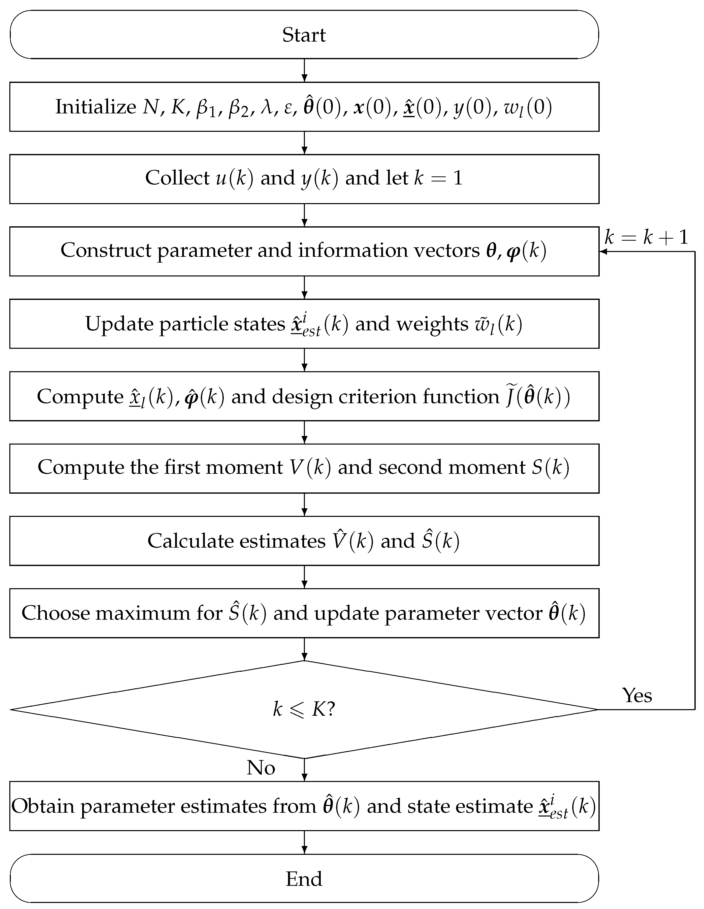
3.3. Joint Estimation Based on Amsgrad-Particle Filter (Ams-PF)

In the gradient calculation of Amsgrad, the vector φ ( k ) contains the unknown states
x ̲ 1 ( k n + 1 ) , , x ̲ n 1 ( k n + 1 ) , x 1 ( k n + 2 ) , , x ̲ n 1 ( k n + 2 ) . These states can be estimated through PF. Meanwhile, the state update in PF includes the matrices E , A , B , whose unknown parameters can be identified by the Amsgrad method. Thus, the PF and the Amsgrad optimization operate alternately during the recursive process to achieve accurate estimation of both system states and parameters.
(1) During the state update process, the parameter estimates based on Amsgrad are obtained. The optimized parameter vector θ ^ ( k ) from Amsgrad contains estimates of all parameters, which means
θ ^ ( k ) = [ a ^ 1 ( k ) , , a ^ n 1 ( k ) , e ^ 1 ( k ) , , e ^ n 1 ( k ) , b ^ 1 ( k ) , , b ^ n 1 ( k ) 1 ] T .
These parameter estimates are used to update the states in PF, that is
E ^ ( k ) D α x ̲ ^ i ( k + 1 ) = A ^ ( k ) x ̲ ^ i ( k ) + B ^ ( k ) u ( k ) .
where E ^ ( k ) , A ^ ( k ) , B ^ ( k ) are estimates of the state transition, control and output matrices, respectively. They are constructed as follows:
E ^ ( k ) = 1 0 0 0 0 1 0 0 0 0 1 0 e ^ 1 ( k ) e ^ 2 ( k ) e ^ n 1 ( k ) 0 R n × n , A ^ ( k ) = 0 1 0 0 0 0 1 0 a ^ 1 ( k ) a ^ 2 ( k ) a ^ n 1 ( k ) 1 0 0 0 1 R n × n , B ^ ( k ) = [ b ^ 1 ( k ) , b ^ 2 ( k ) , , b ^ n 1 ( k ) , 1 ] T R n .
The updated state vector x ̲ ^ e s t i ( k ) is calculated as follows:
x ̲ ^ n e x t i ( k ) = A ^ ( k ) x ̲ ^ i ( k 1 ) + B ^ ( k ) u ( k 1 ) ,
x ̲ ^ e s t i ( k ) = pinv ( E ^ ( k ) ) · x ̲ ^ n e x t i ( k ) ,
x ̲ ^ e s t i ( k ) = x ̲ ^ e s t , 1 i ( k ) , , x ̲ ^ e s t , l i ( k ) , , x ̲ ^ e s t , n i ( k ) T , l = 1 , , n .
The final estimated state is as follows:
x ̲ ^ l ( k ) = 1 N i = 1 N x ̲ ^ e s t , l i ( k ) .
(2) During the Amsgrad optimization process, we also utilize the updated φ ^ ( k ) obtained from PF as
φ ^ ( k ) = [ x ̲ ^ 1 ( k n + 1 ) , , x ̲ ^ n 1 ( k n + 1 ) , x ̲ ^ 1 ( k n + 2 ) , , x ̲ ^ n 1 ( k n + 2 ) , u ( k 1 ) , , u ( k n + 1 ) ] T R 3 ( n 1 ) ,
The new criterion function is defined as follows:
J ˜ ( θ ^ ( k ) ) = 1 2 [ y ( k ) φ ^ T ( k ) θ ^ ( k ) ] 2 ,
The gradient expression of (24) with respect to θ ^ ( k ) becomes
J ˜ ( θ ^ ( k ) ) = J ˜ ( θ ^ ( k ) ) θ ^ ( k ) = φ ^ ( k ) [ y ( k ) φ ^ T ( k ) θ ^ ( k ) ] .
The following optimization process is as described in Section 3.1.
(3) At each time step, the PF and the Amsgrad optimization alternate iteratively. The joint Amsgrad and particle filter (Ams-PF) algorithm operates through the following steps to identify fractional-order singular systems:
  • Initialize the particle number N, the recursion count K, and set parameters β 1 , β 2 , λ and ε . Small initial variables are defined as θ ^ ( 0 ) = 1 3 ( n 1 ) / p 0 , x ( 0 ) = x ̲ ^ ( 0 ) = 1 n / p 0 ,   y ( 0 ) = 1 / p 0 , w l ( 0 ) = 1 / p 0 , p 0 is a relatively large number.
  • Collect u ( k ) and y ( k ) , then set k = 1 . Construct parameter and information vectors θ , φ ( k ) by (7) and (8).
  • The system states based on the PF phase begins. Firstly, solutions of N particles are initialized according to (9). Then, update both the particle weights and states using (13), (20) and (21), and implement the resampling strategy. Finally, the particle weights are normalized to recursively obtain the state estimates x ̲ ^ l ( k ) by (22).
  • Construct the information vector estimate φ ^ ( k ) based on (23). Design the criterion function J ˜ ( θ ^ ( k ) ) according to (24) and compute its gradient value J ˜ ( θ ^ ( k ) ) using (25).
  • In the Amsgrad optimization phase, the system parameters are optimized. Firstly, the first moment V ( k ) and second moment S ( k ) are computed using (14) and (16), respectively. The parameter estimates are updated via gradient information, ensuring the system output converges closer to the true observed values. Then, compute the bias-corrected first moment estimate V ^ ( k ) by (15) and the bias-corrected second moment estimate S ^ ( k ) by (17). Besides, perform the maximum value operation based on (18). Finally, calculate the estimated parameter vector θ ^ ( k ) by (19).
  • Increase k by 1 and return to Step 3. Continue the recursive computation until k reaches the total data length K.
The combined approach benefits from the PF’s capability to efficiently estimate states in nonlinear and high-dimensional systems, while the Amsgrad optimization ensures stable and effective joint estimation through adaptive learning rate adjustment and gradient estimation. In summary, Figure 1 exhibits the flowchart of Ams-PF.
Remark 2.
The traditional gradient descent method is relatively sensitive to the initial parameters. If the initial particle distribution deviates too far from the true parameters, it may lead to convergence to a local optimum or divergence. Amsgrad retains the exponential moving average of the squares of historical gradients and prevents premature decay of the learning rate through maximum value constraints. In the parameter estimation stage, even if the initial particle distribution is poor, this mechanism can more stably adjust the parameter update step size and gradually correct the direction through long-term gradient information. In the joint optimization, the parameter estimation error propagates to the prediction stage of the particle filter through the state transition equation. Amsgrad reduces the dominant influence of the initial large gradient on subsequent updates by adaptively normalizing the parameter gradient, making the parameter estimation process more dependent on long-term statistical features rather than initial randomness.

3.4. Convergence and Error Bound Proof of the Ams-PF Algorithm

The following premise assumptions are given:
(1) For any k, J ˜ ( θ ^ ( k ) ) is a convex function of θ ^ ( k ) ;
(2) For any dimension j of the parameter vector, they are bounded as
θ j θ ^ j ( k ) 2 D j , θ j , θ ^ j ( k ) ;
(3) For any dimension j of the gradient, they are bounded as
J ˜ j ( θ ^ ( k ) ) 2 G j , t .
Let θ * = arg m i n θ ^ k = 1 K J ˜ ( θ ^ ( k ) ) . The indicator for determining convergence is the statistic Regret R ( K ) [32]:
R ( K ) = k = 1 K J ˜ ( θ ^ ( k ) ) J ˜ ( θ * ) .
Because J ˜ ( θ ^ ( k ) ) is a convex function, there is
J ˜ ( θ * ) J ˜ ( θ ^ ( k ) ) + J ˜ ( θ ^ ( k ) ) , θ ^ ( k ) θ * .
Substituting in R ( K ) yields
R ( K ) k = 1 K J ˜ ( θ ^ ( k ) ) , θ ^ ( k ) θ * .
We further split the above equation according to the variable dimensions and change the summation order to obtain
R ( K ) j = 1 3 ( n 1 ) k = 1 K J ˜ j ( θ ^ ( k ) ) ( θ ^ j ( k ) θ j * ) ,
where J ˜ i ( θ ^ ( k ) ) is as follows:
J ˜ j ( θ ^ ( k ) ) = J ˜ ( θ ^ ( k ) ) θ j ^ ( k ) = φ ^ j ( k ) y ( k ) φ ^ j T ( k ) θ ^ j ( k ) .
If we define a new term [33]
γ ( k ) = λ ( k ) 1 1 Π s = 1 k β 1 ( s ) ,
and ignore the small constant ε , the parameter update becomes
θ ^ j ( k + 1 ) = θ ^ j ( k ) γ ( k ) β 1 ( k ) V j ( k 1 ) + ( 1 β 1 ( k ) ) J ˜ j ( θ ^ ( k ) ) S ^ j ( k ) .
Separating the summation terms of (26) can obtain the following:
J ˜ j ( θ ^ ( k ) ) ( θ ^ j ( k ) θ j * ) = S ^ j ( k ) θ ^ j ( k ) θ j * 2 θ ^ j ( k + 1 ) θ j * 2 2 γ ( k ) 1 β 1 ( k ) ( 1 ) β 1 ( k ) 1 β 1 ( k ) V j ( k 1 ) θ ^ j ( k ) θ j * ( 2 ) + γ ( k ) 2 1 β 1 ( k ) V j ( k ) 2 S ^ j ( k ) ( 3 ) .
By expanding and contracting items (1), (2), (3) in (27), we derive that [34]
k = 1 K S ^ j ( k ) θ ^ j ( k ) θ j * 2 θ ^ j ( k + 1 ) θ j * 2 2 γ ( k ) 1 β 1 ( k ) D j 2 G j 2 λ ( K ) 1 β 1 ( 1 ) ,
k = 1 K β 1 ( k ) 1 β 1 ( k ) V j ( k 1 ) θ ^ j ( k ) θ j * G j D j k = 1 K β 1 ( k ) 1 β 1 ( k ) ,
k = 1 K γ ( k ) 2 1 β 1 ( k ) V j ( k ) 2 S ^ j ( k ) k = 1 K γ ( k ) 2 ( 1 β 1 ( k ) ) · r = 1 k ( 1 β 1 ( r ) ) 2 s = r + 1 k β 1 ( s ) 2 ( 1 β 2 ) β 2 k r · G j .
Thus, the upper bound of R ( K ) can be sorted out
R ( K ) j = 1 3 ( n 1 ) D j 2 G j 2 λ ( K ) 1 β 1 ( 1 ) + j = 1 3 ( n 1 ) G j D j k = 1 K β 1 ( k ) 1 β 1 ( k ) + j = 1 3 ( n 1 ) G j k = 1 K γ ( k ) 2 ( 1 β 1 ( k ) ) · r = 1 k ( 1 β 1 ( r ) ) 2 s = r + 1 k β 1 ( s ) 2 ( 1 β 2 ) β 2 k r .
According to the hyperparameters β 1 ( k ) in (14) and β 2 in (16), there are [24]
j = 1 3 ( n 1 ) G j D j k = 1 K β 1 ( k ) 1 β 1 ( k ) j = 1 3 ( n 1 ) G j D j 1 1 β 1 ( 1 ) k = 1 K β 1 ( k ) ,
j = 1 3 ( n 1 ) G j k = 1 K γ ( k ) 2 ( 1 β 1 ( k ) ) · r = 1 k ( 1 β 1 ( r ) ) 2 s = r + 1 k β 1 ( s ) 2 ( 1 β 2 ) β 2 k r j = 1 3 ( n 1 ) G j · k = 1 K λ ( k ) 2 ( 1 β 1 ( 1 ) ) 2 ( 1 β 2 ) ( 1 c ) .
From (28)–(30), we find that the order of magnitude of the upper bound of R ( K ) is only related to 1 λ ( K ) , k = 1 K β 1 ( k ) , and k = 1 K λ ( k ) . Because λ ( k ) = λ k , then
1 λ ( K ) = O ( K 1 2 ) , k = 1 K λ ( k ) = O ( K 1 2 ) .
Moreover, due to β 1 ( k ) = β 1 k , there is
k = 1 K β 1 ( k ) = O ( K 1 2 ) .
It can be seen by (31) and (32) that the upper order of R ( K ) is maintained at the optimal state ( K 1 2 ) . Thus, the average amortization value R ( K ) / K = O ( K 1 2 ) tends to 0 when K [35].
After Amsgrad optimization, the error of PF usually refers to the difference between the empirical distribution p ^ N = p ( x ̲ l i ( k ) | y ( 1 : K ) , u ( 1 : K ) , θ ^ ( k 1 ) ) based on θ ^ ( k 1 ) and the true posterior distribution p = p ( x ̲ l i ( k ) | y ( 1 : K ) , u ( 1 : K ) ) . For a particle set { x ̲ l i ( 1 : k ) , w l i ( k ) } i = 1 N before resampling, the empirical distribution is computed by (10). The weights follow [16]
w l i ( k ) p ( X l i ( k ) , Y ( k ) ) d ( X l i ( k ) | Y ( k ) ) .
The resampling operation generates an equally weighted particle set { x ̲ l j ( 1 : k ) , 1 N } j = 1 N from p ^ N , corresponding to the resampled empirical distribution [17]:
p ^ N res = p ^ ( x ̲ l j ( k ) | y ( 1 : K ) , u ( 1 : K ) , θ ^ ( k 1 ) ) 1 N j = 1 N Δ ( x ̲ l j ( k ) x ̲ ^ l j ( k ) ) .
Decompose the total error into
p ^ N res p p ^ N res p ^ N + p ^ N p ,
where p ^ N res p ^ N is the resampling error and p ^ N p is the initial sampling error.
Lemma 1.
Under the condition that the importance weights have finite variance ( Var ( w l i ( k ) ) < ), and for any bounded function J ˜ ( J ˜ 1 ), the error of the classical PF is [36]
E ( p ^ N ( J ˜ ) p ( J ˜ ) ) 2 Var ( w l ( k ) ) · J ˜ 2 N .
Proof. 
Based on the properties of importance sampling and the law of large numbers, there is
p ^ N ( J ˜ ) = i = 1 N w l i ( k ) J ˜ ( x ̲ l i ( 1 : k ) ) , E [ p ^ N ( J ˜ ) ] = p ( J ˜ ) .
By combining (33), the variance is calculated as
Var ( p ^ N ( J ˜ ) ) = 1 N Var q ( w l ( k ) J ˜ ) E q [ w l 2 ( k ) J ˜ 2 ] N Var ( w l ( k ) ) · J ˜ 2 N .
Lemma 2.
For any bounded function J ˜ ( J ˜ 1 ) , the empirical distribution after resampling satisfies [37]
E ( p ^ N res ( J ˜ ) p ^ N ( J ˜ ) ) 2 | p ^ N J ˜ 2 N .
Proof. 
After resampling, particle x ̲ l j ( 1 : k ) is conditionally independent and identically distributed from p ^ N , there is
E p ^ N res ( J ˜ ) | p ^ N = p ^ N ( J ˜ ) , Var p ^ N res ( J ˜ ) | p ^ N = Var p ^ N ( J ˜ ) N J ˜ 2 N .
Using Lemma 2 and the law of total expectation, the expectation of resampling error is
E ( p ^ N res ( J ˜ ) p ^ N ( J ˜ ) ) 2 = E E ( p ^ N res ( J ˜ ) p ^ N ( J ˜ ) ) 2 | p ^ N J ˜ 2 N .
The mean square bound of the total error is obtained by combining Lemma 1 and resampling error:
E ( p ^ N res ( J ˜ ) p ( J ˜ ) ) 2 2 E ( p ^ N res ( J ˜ ) p ^ N ( J ˜ ) ) 2 + E ( p ^ N ( J ˜ ) p ( J ˜ ) ) 2 2 1 + Var ( w l ( k ) ) · J ˜ 2 N .
The upper bound of the total variation error is derived through the Jensen inequality and the total variation norm ( · TV ):
E p ^ N res p TV p ^ N res p TV 2 2 1 + Var ( w l ( k ) ) · J ˜ 2 N .
If we define the difference between the initial particle distribution and the true distribution as F 0 , and let F = F 0 · 2 1 + Var ( w l ( k ) ) · J ˜ 2 , the error constant F ( k ) increases exponentially due to the mixality of state transitions for the k-step filtering:
F ( k ) F · ζ k , ζ > 1 .
In summary, the upper bound of Ams-PF error can be concluded as follows:
Theorem 1.
Let the resampling PF method under the following conditions:
(1) The variance of the importance weight is limited.
(2) The resampling algorithm is unbiased.
(3) The state transition model has exponential mixing.
Then, for any bounded function J ˜ ( J ˜ 1 ) , there exists a constant F and ζ > 1 , such that the upper bound of the resampling PF error is
E p ^ N res p TV F ζ k N .

4. Illustrative Examples

In this section, two examples, including a third-order singular system and a fourth-order singular system with fractional orders, are presented to evaluate the effectiveness. After each joint estimation process of Ams-PF, the system’s parameter vector and state vector are updated. To assess the performance of parameter identification and state estimation, the updating process monitors optimization progress by calculating the parameter estimation error at each recursion step.
The calculations and graphs are performed on MATLAB® 2022b in simulation. Finally, the optimization results are visualized through tables and graphical representations, demonstrating the variation trend of parameter estimation errors with the recursion time. These results prove that the joint estimation algorithm can stably converge to the vicinity of true values after multiple recursion cycles.

4.1. Three-Order Fractional Singular System

Consider the following three-order singular system with the state transition, control and output matrices defined, respectively, as follows:
E = 1 0 0 0 1 0 1.45 7.62 0 , A = 0 1 0 1.29 7.5 1 0 0 1 , B = 12.23 10.85 1 .
The fractional order is α = 0.2 . The parameter vector of this three-order singular system is
θ = [ e 1 , e 2 , a 1 , a 2 , b 1 , b 2 ] T = [ 1.45 , 7.62 , 1.29 , 7.5 , 12.23 , 10.85 ] T .
The variation range of parameters in the system matrix is [−20, 20], and they can be positive or negative during the optimization process. To quantify the discrepancy between identified results and true parameters, the parameter estimation error is defined as follows:
δ = θ ^ ( k ) θ θ ,
where θ ^ ( k ) represents the parameter identification results based on the Ams-PF, θ contains the true values of system parameters.
The input u ( k ) of the three-order singular system is the uncorrelated measurable random signal sequence with zero mean and unit variance, and the noise v ( k ) is the zero-mean Gaussian sequence with variance σ 2 = 0 . 8 2 . The proposed Ams-PF is used to identify this three-order singular system. Table 1 shows partial parameter estimates and error values. Figure 2 shows the variation curve of parameter estimation errors. Figure 3 presents the boxplot of each parameter estimation, and Figure 4 denotes a comparison between the estimated parameters and the true values of Ams-PF. The state and output fitting curves of the system are shown in Figure 5 and Figure 6, respectively. To prove the robustness of the algorithm, we conduct simulations at two higher noise levels, and the results are shown in Table 2 and Figure 7. Furthermore, parameters and states of the above system are estimated using the Amsgrad, PF and Gravitational search algorithm-Kalman filter (GSA-KF) methods. The estimation results are also displayed in Table 1, Figure 2, Figure 5 and Figure 6.

4.2. Four-Order Fractional Singular System

Here we further consider a four-order singular system with the following state transition, control and output matrices:
E = 1 0 0 0 0 1 0 0 0 0 1 0 4.35 5.6 3.22 0 , A = 0 1 0 0 0 0 1 0 4.30 5.55 3.17 1 0 0 0 1 , B = 0.38 6.5 1.33 1 .
The fractional order is α = 0.1 . The parameter vector of the four-order singular system is defined as follows:
θ = [ e 1 , e 2 , e 3 , a 1 , a 2 , a 3 , b 1 , b 2 , b 3 ] T = [ 4.35 , 5.6 , 3.22 , 4.30 , 5.55 , 3.17 , 0.38 , 6.5 , 1.33 ] T .
Different from Example 4.1, the variance in noise v ( k ) is set as σ 2 = 0 . 6 2 . The proposed Ams-PF, Amsgrad, PF and GSA-KF algorithms are employed to estimate both parameters and states in this four-order singular system. The results are shown in Table 3 and Figure 8, Figure 9, Figure 10 and Figure 11. To verify the robustness under parameter uncertainty, we conduct 10 Monte Carlo experiments under the initial value uncertainty. The average values and standard deviations of Ams-PF are demonstrated by Table 4.
From Table 1, Table 2, Table 3 and Table 4 and Figure 2, Figure 3, Figure 4, Figure 5, Figure 6, Figure 7, Figure 8, Figure 9, Figure 10 and Figure 11, we can draw the following conclusions:
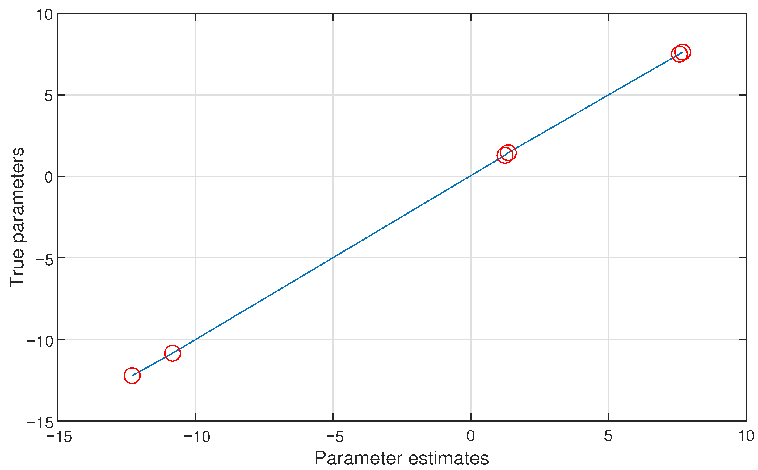
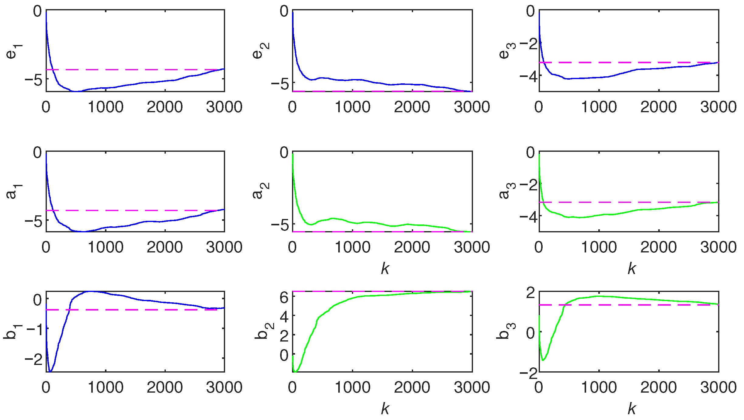
  • By horizontally looking at the values in Table 1 and Table 3, it can be observed that the parameters identified by Ams-PF gradually approach the true values as k increases. It can be seen from the last line of each method that the final identification errors of Ams-PF are 0.77586 and 0.99473 , which are significantly smaller than those of the Amsgrad ( 55.51342 and 61.68410 ) and GSA-KF ( 40.03237 and 46.87218 ) methods. Thus, the Ams-PF algorithm can effectively identify fractional singular systems and its identification performance is satisfactory.
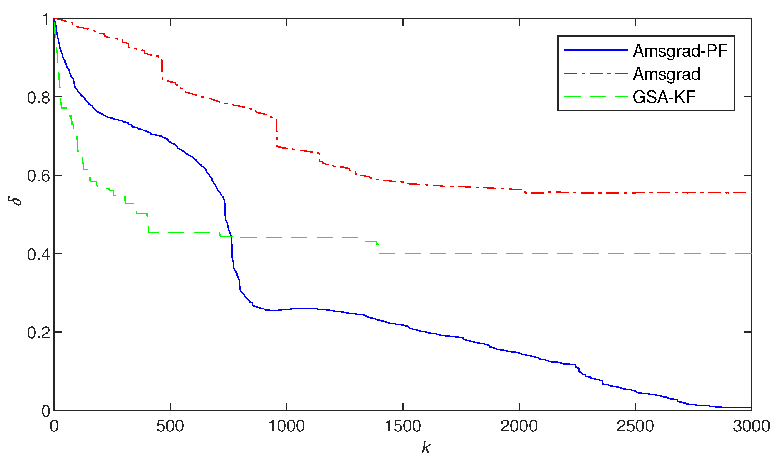
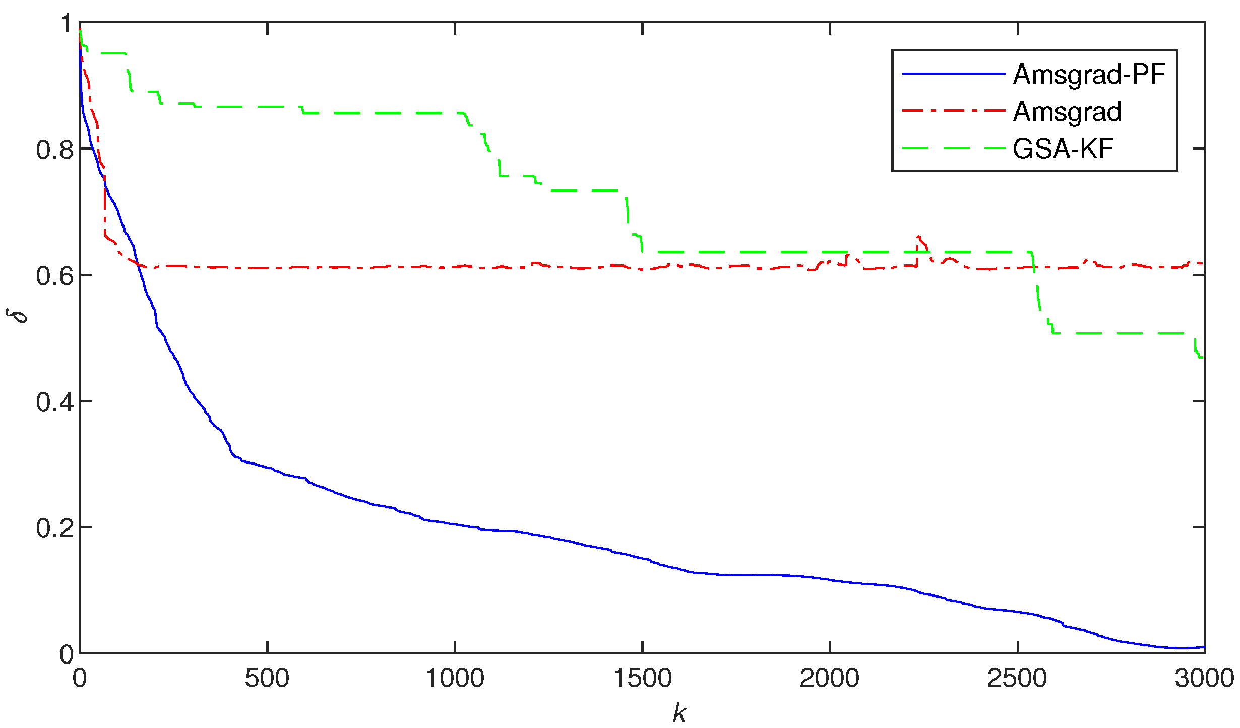
  • In Figure 2, Figure 3 and Figure 4, Figure 8 and Figure 9, the Ams-PF algorithm exhibits excellent convergence speed and identification accuracy. Moreover, the system parameters identified by Ams-PF all converge near their true values with minimal estimation errors. Thus, it exhibits a stronger ability to escape local optima and has a faster convergence speed than Amsgrad and GSA-KF.
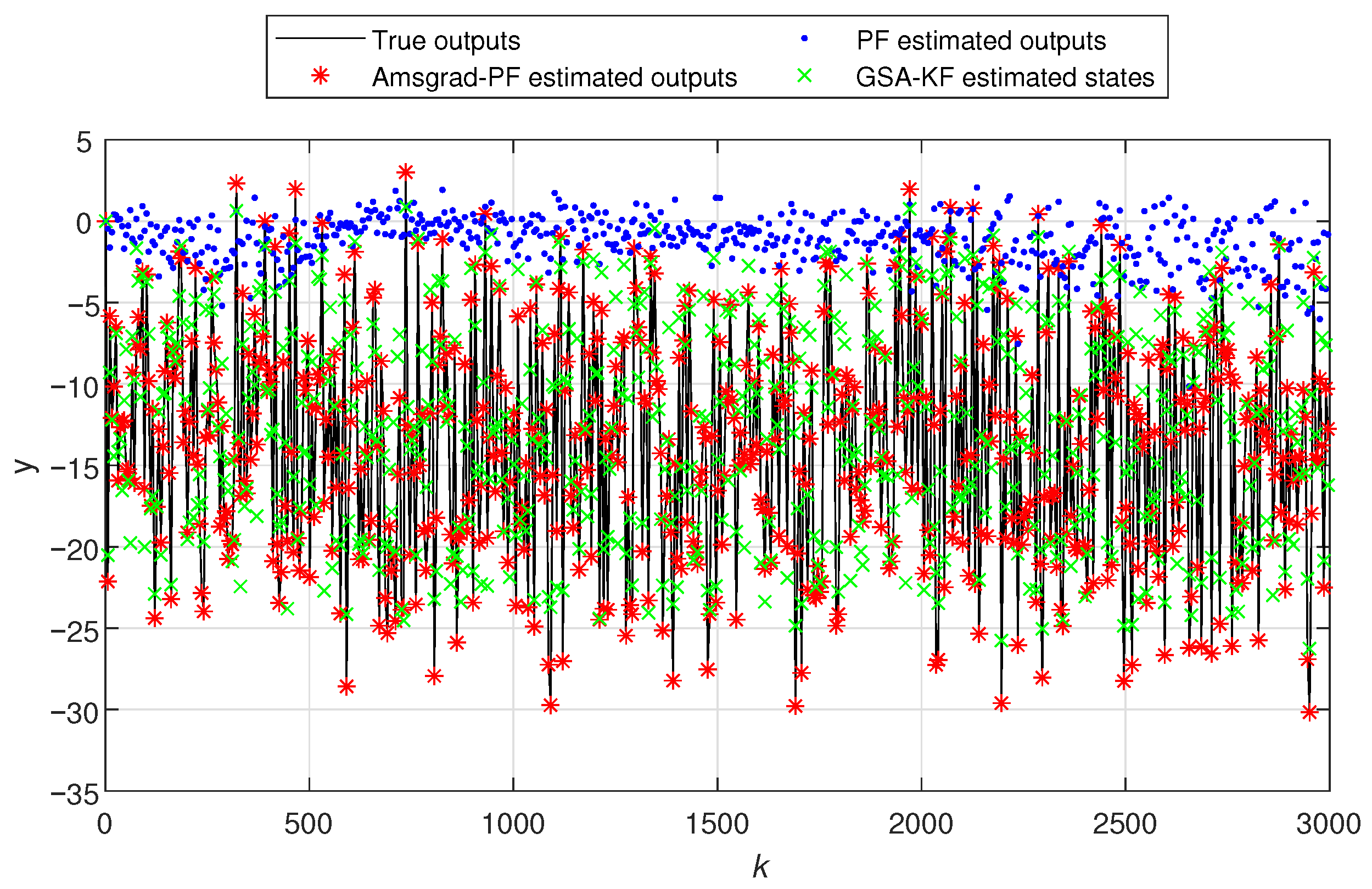
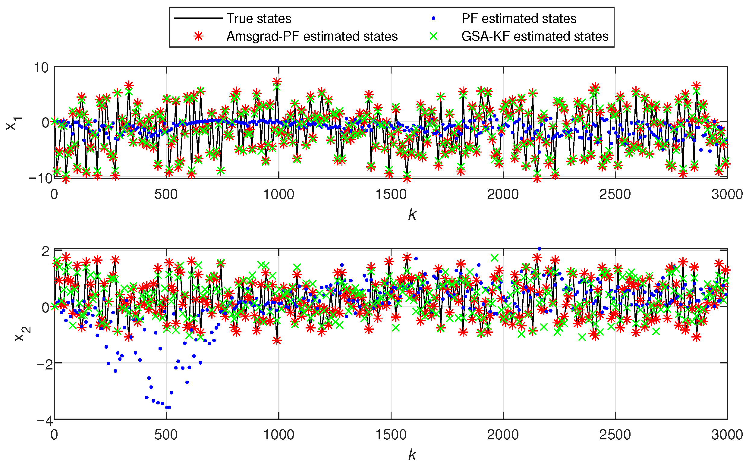
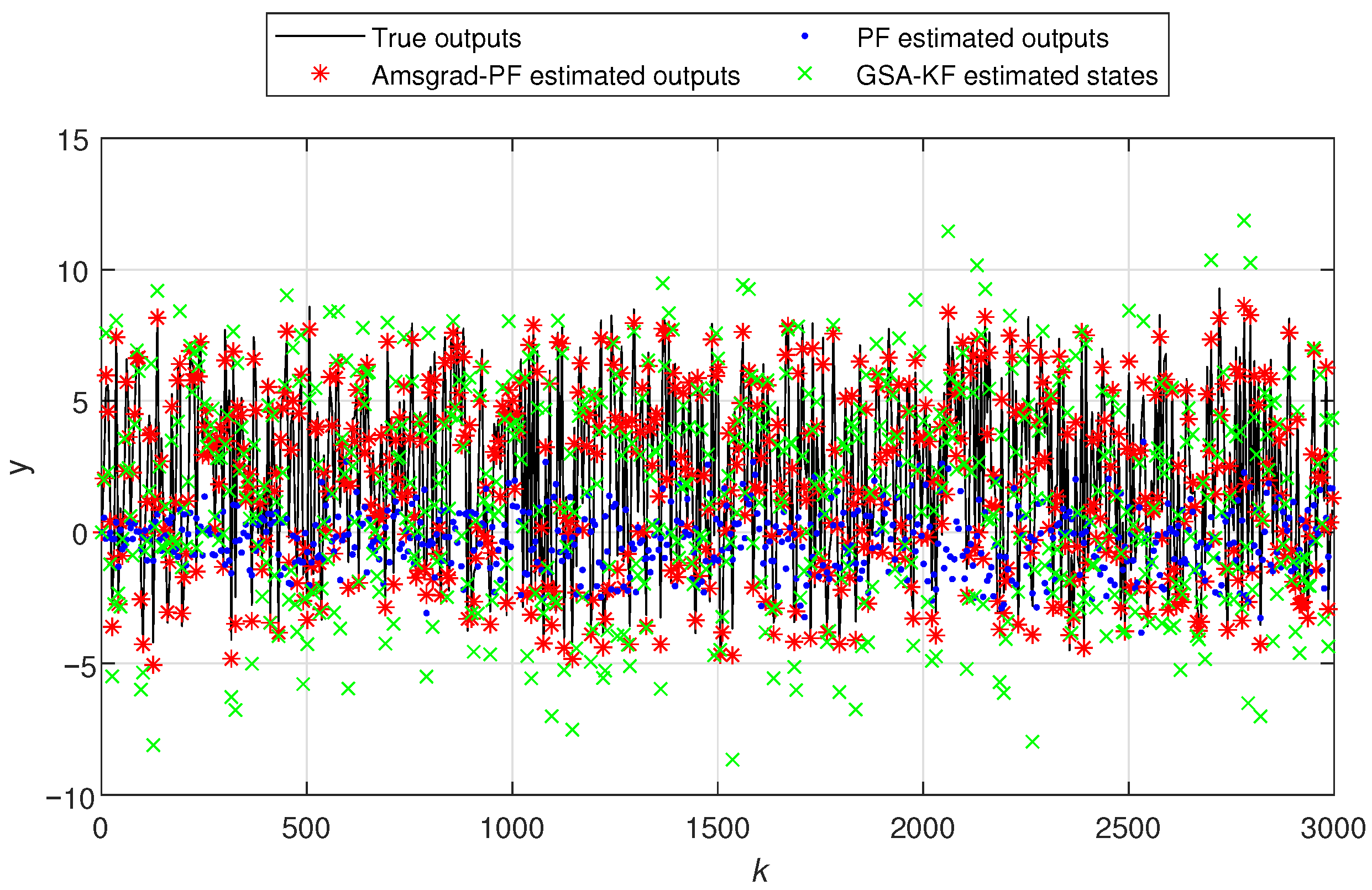
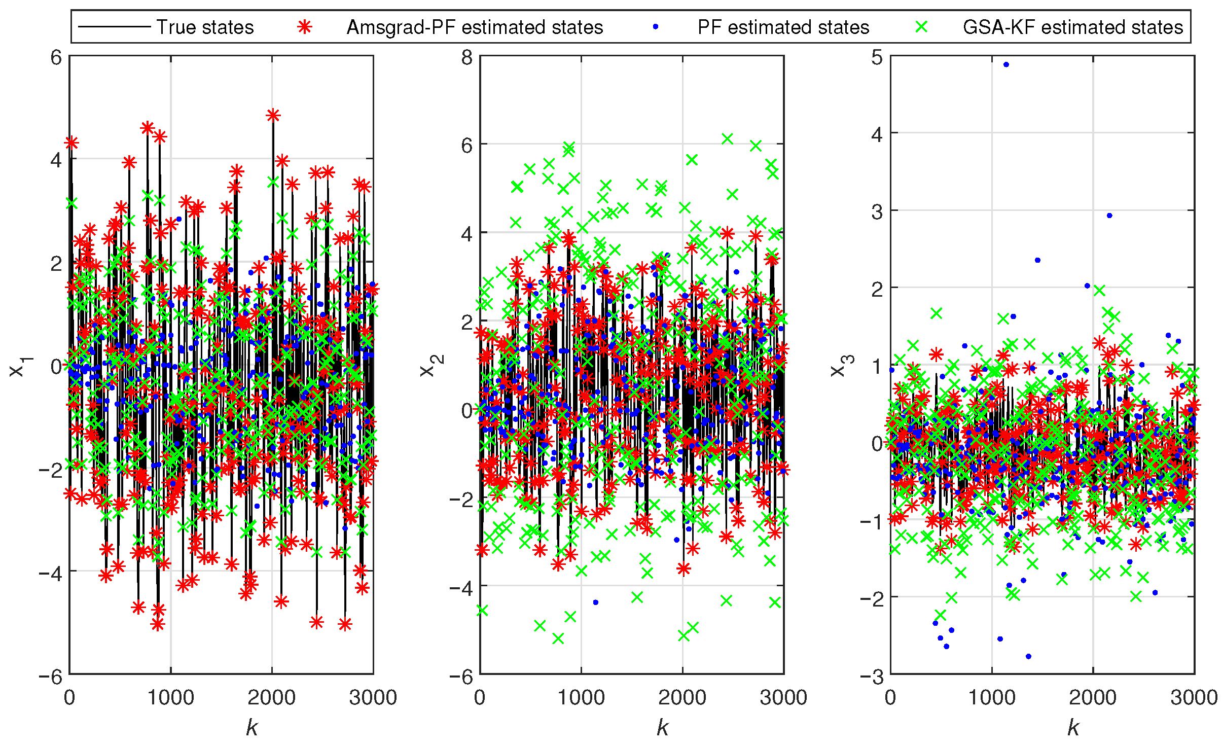
  • In Figure 5 and Figure 10, the black line represents the true output, the red stars indicate the estimated outputs of Ams-PF, the blue dots represent the estimated outputs of PF, and the green forks denote the estimated outputs of GSA-KF. The system states in Figure 6 and Figure 11 are the same. As can be seen from these figures, the red stars are closest to the black line, which means that the estimated outputs and states of Ams-PF have a best fit with the true output and state values. These performances further demonstrate that the Ams-PF algorithm achieves satisfactory fitting between estimated and actual states, estimated outputs and actual outputs. The fitting performance is excellent and clearly superior to that of the PF and GSA-KF. Thus, the Ams-PF algorithm can effectively accomplish state estimation for fractional singular systems.
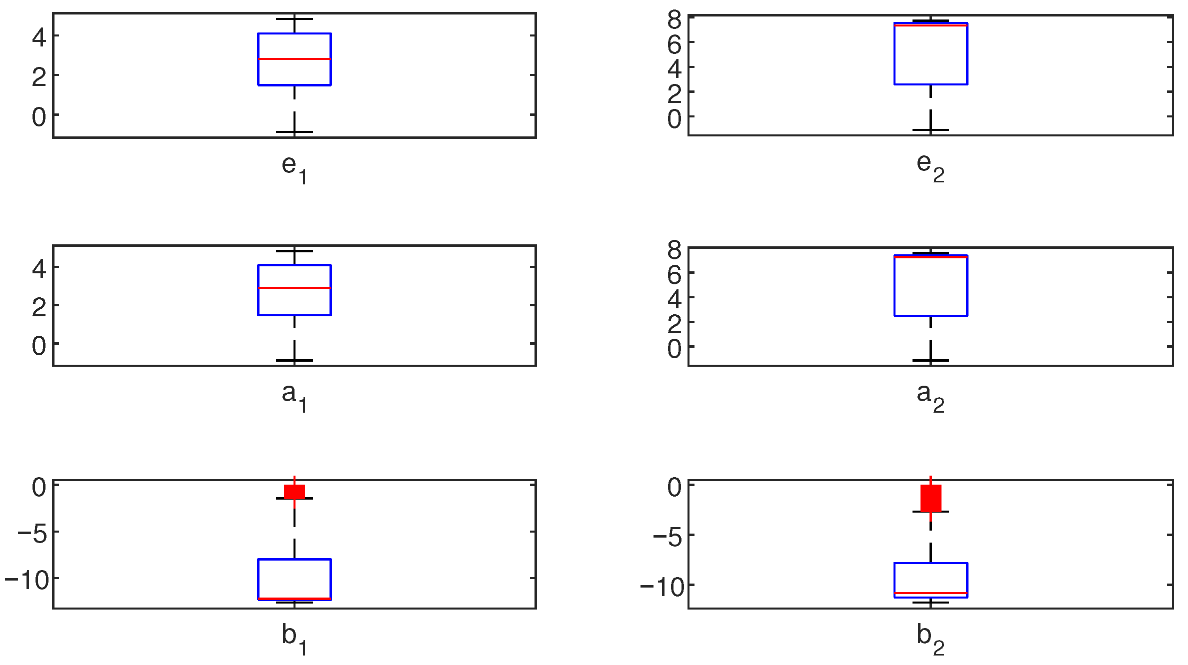
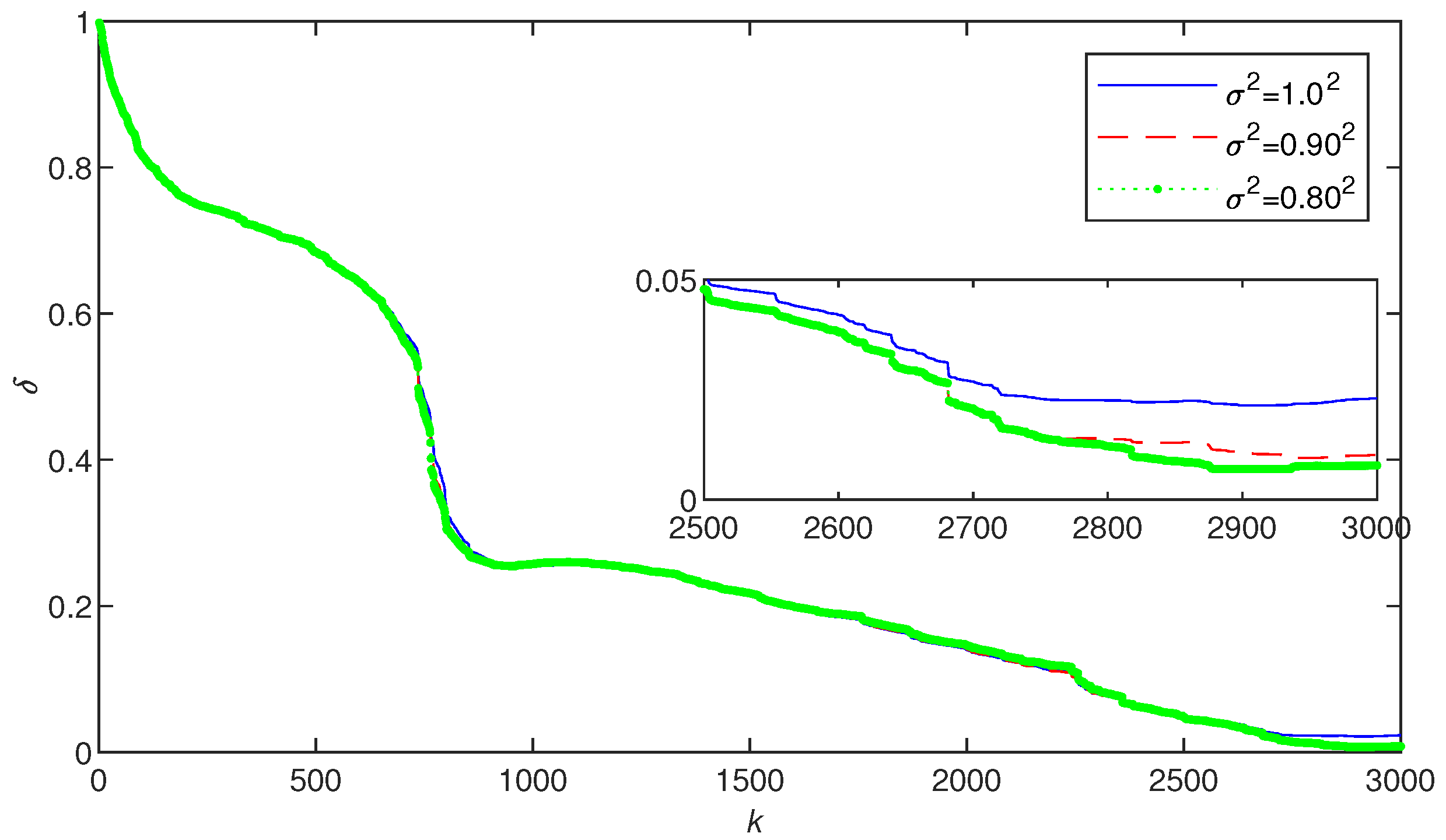
  • From Table 2 and Figure 7, it can be seen that as the noise variance increases, the parameter estimation error becomes larger. However, this change is very minor. In Table 4, the final average value of Ams-PF identification error is 1.15654 and the standard deviation is 0.30091. Thus, we can conclude that the Ams-PF method can guarantee a certain robustness under different noise interferences or parameter uncertainty.

5. Conclusions

Singular systems have been widely applied in multiple fields, including control engineering, economic management, chemical processes, communication networks, and aerospace systems. Fractional-order singular systems are becoming increasingly important because they can approximate many systems with inconsistent speeds. Consequently, the accurate modeling of the fractional singular system becomes particularly important. This paper proposes an Ams-PF algorithm for joint parameter and state estimation of some fractional singular systems. The Amsgrad algorithm is computationally efficient and possesses strong optimization capability. Due to its powerful parallel search ability, it can effectively identify multiple parameters in singular systems. The PF algorithm approximates the probability density function by propagating random samples in the state space and uses the sample mean instead of the integration operation. Thus, minimum variance estimates of singular system states are obtained. By combining these advantages, the proposed Ams-PF algorithm can accelerate parameter convergence speed and improve estimation accuracy. Meanwhile, it can handle the relationship between states and parameters in fractional singular systems and enhance the overall joint estimation performance. Two simulation examples demonstrate that the Ams-PF achieves high estimation accuracy, fast convergence speed and excellent identification performance. Therefore, the Ams-PF algorithm can effectively identify fractional singular systems by delivering superior state estimation results and demonstrating significant practical application value.

Author Contributions

Conceptualization, K.Z.; Methodology, K.Z.; Software, Z.W.; Validation, Z.W.; Formal analysis, T.Z.; Investigation, K.Z.; Resources, T.S.; Data curation, T.Z.; Writing – original draft, T.S.; Writing – review and editing, K.Z. and T.Z.; Visualization, Z.W.; Supervision, T.S.; Project administration, T.S.; Funding acquisition, T.Z. All authors have read and agreed to the published version of the manuscript.

Funding

This work was supported in part by the National Natural Science Foundation of China (62473215), and the Natural Science Foundation of Nantong City (JC2023064, JC2023006).

Data Availability Statement

The original contributions presented in this study are included in the article. Further inquiries can be directed to the corresponding author.

Conflicts of Interest

The authors declare no conflicts of interest.

Abbreviations

The following abbreviations are used in this manuscript:
PFParticle Filter
Ams-PFAmsgrad-Particle Filter
AdamAdaptive Moment Estimation
GLGrünwald–Letnikov
GSA-KFGravitational Search Algorithm-Kalman Filter

References

  1. Alsaedi, R. Existence results related to a singular fractional double-phase problem in the whole space. Fractal Fract. 2024, 8, 292. [Google Scholar] [CrossRef]
  2. Liu, X.; Yang, R. Predefined-time adaptive robust control of a class of nonlinear singular systems. Proc. Inst. Mech. Eng. Part J. Syst. Control Eng. 2024, 239, 3–15. [Google Scholar] [CrossRef]
  3. Li, H.; Zhou, B.; Michiels, W. Prescribed-time unknown input observers design for singular systems: A periodic delayed output approach. IEEE Trans. Syst. Man Cybern. Syst. 2023, 54, 741–751. [Google Scholar] [CrossRef]
  4. Hong, L.; Zhang, N. On the preconditioned MINRES method for solving singular linear systems. Comput. Appl. Math. 2022, 41, 1007–1026. [Google Scholar] [CrossRef]
  5. Zhang, Z.; Li, Y. Global classical solutions of a nonlinear consumption system with singular density-suppressed motility. Appl. Math. Lett. 2024, 151, 1021–1034. [Google Scholar] [CrossRef]
  6. Zhang, Q.; Lu, J. H control for singular fractional-order interval systems. ISA Trans. 2021, 110, 105–106. [Google Scholar] [CrossRef] [PubMed]
  7. Shu, Y.; Li, B.; Zhu, Y. Optimal control for uncertain discrete-time singular systems under expected value criterion. Fuzzy Optim. Decis. Mak. 2020, 20, 331–364. [Google Scholar] [CrossRef]
  8. Liu, R.; Chang, X.; Chen, Z. Dissipative control for switched nonlinear singular systems with dynamic quantization. Commun. Nonlinear Sci. Numer. Simul. 2023, 127, 102–108. [Google Scholar] [CrossRef]
  9. Zhang, Y.; Mu, X. Event-triggered output quantized control of discrete Markovian singular systems. Automatica 2022, 135, 109–110. [Google Scholar] [CrossRef]
  10. Allahverdiev, B.; Tuna, H. Singular discontinuous Hamiltonian systems. J. Appl. Anal. Comput. 2022, 12, 1386–1402. [Google Scholar] [CrossRef] [PubMed]
  11. Ristic, B.; Houssineau, J. Robust target motion analysis using the possibility particle filter. IET Radar Sonar Navig. 2019, 13, 18–22. [Google Scholar] [CrossRef]
  12. Liu, Y.; Shi, Q.; Wei, Y. State of charge estimation by square root cubature particle filter approach with fractional order model of lithium-ion battery. Sci. China-Technol. Sci. 2022, 65, 1760–1771. [Google Scholar] [CrossRef]
  13. Xie, X.; Du, J.; Wu, J. Adaptive particle filter for change point detection of profile data in manufacturing systems. IEEE Trans. Autom. Sci. Eng. 2024, 21, 7143–7157. [Google Scholar] [CrossRef]
  14. Michalski, J.; Kozierski, P. MultiPDF particle filtering in state estimation of nonlinear objects. Nonlinear Dyn. 2021, 106, 2165–2182. [Google Scholar] [CrossRef]
  15. Abolmasoumi, A.; Farahani, A.; Mili, L. Robust particle filter design with an application to power system state estimation. IEEE Trans. Power Syst. 2024, 39, 1810–1821. [Google Scholar] [CrossRef]
  16. Bao, F.; Cao, Y.; Han, X. An implicit algorithm of solving nonlinear filtering problems. Commun. Comput. Phys. 2014, 16, 382–402. [Google Scholar] [CrossRef]
  17. Kang, J.; Chen, X.; Tao, Y. Optimal transportation particle filter for linear filtering systems with correlated noises. IEEE Trans. Aerosp. Electron. Syst. 2023, 58, 5190–5203. [Google Scholar] [CrossRef]
  18. Waseem; Ullah, A.; Awwad, F.; Ismail, E. Analysis of the corneal geometry of the human eye with an artificial neural network. Fractal Fract. 2023, 7, 764. [Google Scholar] [CrossRef]
  19. Wang, L.; Liu, Z. Data-driven product design evaluation method based on multi-stage artificial neural network. Appl. Soft Comput. 2021, 103, 1302–1317. [Google Scholar] [CrossRef]
  20. Chang, Z.; Zhang, Y.; Chen, W. Electricity price prediction based on hybrid model of adam optimized LSTM neural network and wavelet transform. Energy 2019, 187, 1000–1016. [Google Scholar] [CrossRef]
  21. Chen, H.; Shi, Y.; Zhang, J.; Zhao, Y. Sharp error estimate of a Grünwald–Letnikov scheme for reaction-subdiffusion equations. Numer. Algorithms 2022, 89, 1465–1477. [Google Scholar] [CrossRef]
  22. Zong, T.; Li, J.; Lu, G. Identification of fractional order Wiener-Hammerstein systems based on adaptively fuzzy PSO and data filtering technique. Appl. Intell. 2022, 52, 1–14. [Google Scholar] [CrossRef]
  23. Zhang, Q.; Lu, J. Novel admissibility and robust stabilization conditions for fractional-order singular systems with polytopic uncertainties. Asian J. Control 2024, 26, 70–84. [Google Scholar] [CrossRef]
  24. Tong, Q.; Liang, G.; Bi, J. Calibrating the adaptive learning rate to improve convergence of ADAM. Neurocomputing 2022, 481, 333–356. [Google Scholar] [CrossRef] [PubMed]
  25. Aspeel, A.; Gouverneur, A.; Jungers, R. Optimal intermittent particle filter. IEEE Trans. Signal Process. 2022, 70, 2814–2825. [Google Scholar] [CrossRef]
  26. Zong, T.; Li, J.; Lu, G. Maximum likelihood LM identification based on particle filtering for scarce measurement-data MIMO Hammerstein Box-Jenkins systems. Math. Comput. Simul. 2025, 230, 241–255. [Google Scholar] [CrossRef]
  27. Habibi, Z.; Zayyani, H.; Korki, M. A robust Markovian block sparse adaptive algorithm with its convergence analysis. IEEE Trans. Circuits Syst. Ii Express Briefs 2024, 71, 1546–1550. [Google Scholar] [CrossRef]
  28. Padhy, M.; Vigneshwari, S.; Ratnam, M. Application of empirical Bayes adaptive estimation technique for estimating winds from MST radar covering higher altitudes. Signal Image Video Process. 2023, 17, 3303–3311. [Google Scholar] [CrossRef]
  29. Li, J.; Xiao, K.; Gu, J.; Hua, L. Parameter estimation of multiple-input single-output Hammerstein controlled autoregressive system based on improved adaptive moment estimation algorithm. Int. J. Robust Nonlinear Control 2023, 33, 7094–7113. [Google Scholar] [CrossRef]
  30. Yang, M.; Yue, F.; Lu, B.; Zhao, H.; Ma, G.; Wang, L. Quantum gate control pulse optimization based on the Adam algorithm. Quantum Inf. Process. 2025, 24, 175. [Google Scholar] [CrossRef]
  31. Iqbal, N.; Wang, H.; Zheng, Z.; Yao, M. Reinforcement learning-based heuristic planning for optimized energy management in power-split hybrid electric heavy duty vehicles. Energy 2024, 302, 131773. [Google Scholar] [CrossRef]
  32. Xu, Y.; Xu, Y.; Yan, Y. Parallel and distributed asynchronous adaptive stochastic gradient methods. Math. Program. Comput. 2023, 15, 471–508. [Google Scholar] [CrossRef]
  33. Radhakrishnan, P.; Senthilkumar, G. Nesterov-accelerated adaptive moment estimation NADAM-LSTM based text summarization. J. Intell. Fuzzy Syst. 2024, 46, 6781–6793. [Google Scholar]
  34. Li, X.; Yin, Y.; Feng, R. Double total variation (DTV) regularization and improved adaptive moment estimation (IADAM) optimization method for fast MR image reconstruction. Comput. Methods Programs Biomed. 2023, 233, 6172–6201. [Google Scholar] [CrossRef] [PubMed]
  35. Hu, T.; Liu, X.; Ji, K.; Lei, Y. Convergence of adaptive stochastic mirror descent. IEEE Trans. Neural Netw. Learn. Syst. 2025, 1–12. [Google Scholar] [CrossRef] [PubMed]
  36. Crisan, D.; Doucet, A. A survey of convergence results on particle filtering methods for practitioners. IEEE Trans. Signal Process. 2002, 50, 736–746. [Google Scholar] [CrossRef]
  37. Hu, X.; Schön, T.; Ljung, L. A general convergence result for particle filtering. IEEE Trans. Signal Process. 2011, 59, 3424–3429. [Google Scholar] [CrossRef]
Figure 1. Flowchart of Ams-PF.
Fractalfract 09 00480 g001
Figure 2. Variation curves of identification error versus k in the three-order fractional singular system based on Ams-PF, Amsgrad and GSA-KF.
Fractalfract 09 00480 g002
Figure 3. Boxplot of every parameter estimation in the three-order fractional singular system.
Fractalfract 09 00480 g003
Figure 4. Comparison between the estimated parameters and the true values of Ams-PF.
Fractalfract 09 00480 g004
Figure 5. Fitting curve of estimated and true outputs in the three-order fractional singular system.
Fractalfract 09 00480 g005
Figure 6. Fitting curves of estimated and true state components in the three-order fractional singular system.
Fractalfract 09 00480 g006
Figure 7. Identification errors of the three-order fractional singular system based on Ams-PF under various noises.
Fractalfract 09 00480 g007
Figure 8. Variation curves of identification error versus k in the four-order fractional singular system based on Ams-PF, Amsgrad and GSA-KF.
Fractalfract 09 00480 g008
Figure 9. Variation of each parameter estimate versus k in the four-order fractional singular system.
Fractalfract 09 00480 g009
Figure 10. Fitting curve of estimated and true outputs in the four-order fractional singular system.
Fractalfract 09 00480 g010
Figure 11. Fitting curves of estimated and true state components in the four-order fractional singular system.
Fractalfract 09 00480 g011
Table 1. Parameter estimation and errors of the three-order fractional singular system ( σ 2 = 0 . 8 2 ).
AlgorithmParameterk = 100k = 200k = 500k = 1000k = 2000k = 3000True Value
Ams-PF e 1 −0.61541−0.024761.141924.723563.354761.357201.45000
e 2 −1.06909−0.92999−0.245116.489387.482467.681507.62000
a 1 −0.62677−0.019941.181924.738523.422331.237151.29000
a 2 −1.12186−0.97711−0.287726.383957.359427.562797.50000
b 1 −4.49469−5.55102−6.21625−11.97485−12.32042−12.28608−12.23000
b 2 −4.56647−5.58235−6.20746−11.42739−11.01381−10.81964−10.85000
δ ( % ) 81.6777775.7637268.4062325.7389214.630150.775860.00000
Amsgrad e 1 −0.00006−0.00006−0.00007−0.00007−0.00008−0.000091.45000
e 2 −0.00006−0.00006−0.00007−0.00007−0.00008−0.000097.62000
a 1 −0.00006−0.00006−0.00007−0.00007−0.00008−0.000091.29000
a 2 −0.00006−0.00006−0.00007−0.00007−0.00008−0.000097.50000
b 1 −0.32544−0.58082−2.51044−5.70348−10.32070−13.04685−12.23000
b 2 −0.40543−0.70195−3.22139−7.46451−11.53878−10.95777−10.85000
δ ( % ) 97.8377596.2169183.8186766.8342456.3118455.513420.00000
GSA-KF e 1 1.602281.878922.136520.553121.709220.714781.45000
e 2 1.113660.462822.170601.040382.378032.592757.62000
a 1 0.43591−0.224260.78218−0.102660.24588−0.313171.29000
a 2 0.993660.74029−0.333930.82055−0.261980.975897.50000
b 1 −5.61093−6.65074−11.22424−13.54027−13.27158−12.65576−12.23000
b 2 −3.68962−4.99514−9.76241−8.89775−10.09497−8.62924−10.85000
δ ( % ) 68.4379456.6157145.4203844.0123340.0323740.032370.00000
Table 2. Parameter estimation and errors of the three-order fractional singular system based on Ams-PF under different noises.
Noisek e 1 e 2 a 1 a 2 b 1 b 2 δ ( % )
σ 2 = 0 . 9 2 100−0.61993−1.07816−0.63087−1.12662−4.51960−4.5953181.58529
200−0.02616−0.93060−0.02162−0.97967−5.58548−5.6208375.62647
5001.12818−0.251721.16804−0.29629−6.24719−6.2426168.32139
10004.686126.428754.696506.32621−11.92001−11.3828925.59878
20003.269997.445643.357067.30810−12.31156−11.0040514.11934
30001.562267.554201.386927.44336−12.32993−10.860131.01396
σ 2 = 1 . 0 2 100−0.62497−1.07610−0.63717−1.13089−4.57133−4.6510981.37875
200−0.03067−0.93304−0.02977−0.98243−5.64181−5.6818575.41060
5001.10890−0.265371.14559−0.31072−6.29412−6.2948468.21139
10004.611116.312604.616626.21463−11.79260−11.2785025.36458
20003.240967.307393.327947.16698−12.27024−10.9829214.03265
30001.632357.341081.428737.24212−12.31576−10.874922.30512
True Value1.450007.620001.290007.50000−12.23000−10.850000.00000
Table 3. Parameter estimation and errors of the four-order fractional singular system.
AlgorithmParameterk = 100k = 200k = 500k = 1000k = 2000k = 3000True Value
Ams-PF e 1 −4.15262−5.26322−5.93478−5.67812−5.17051−4.28444−4.35000
e 2 −3.89106−4.56233−4.68299−4.80976−5.13349−5.62614−5.60000
e 3 −3.37188−3.87983−4.22355−4.13936−3.58811−3.22194−3.22000
a 1 −4.02288−5.03670−5.81737−5.54977−5.08730−4.22023−4.30000
a 2 −3.91768−4.78959−4.76688−4.92696−5.06612−5.55220−5.55000
a 3 −3.42535−3.75496−4.09824−3.97158−3.57478−3.16901−3.17000
b 1 −2.37429−1.656050.060440.18526−0.13507−0.31770−0.38000
b 2 −1.528450.185784.080405.789426.284966.496796.50000
b 3 −1.30907−0.485741.468461.760741.571581.361581.33000
δ ( % ) 70.3258354.4135629.4161120.4070411.599740.994730.00000
Amsgrad e 1 −2.00252−2.08265−2.09940−2.09940−2.09940−2.09941−4.35000
e 2 −2.00252−2.08265−2.09940−2.09940−2.09940−2.09941−5.60000
e 3 −2.00252−2.08265−2.09940−2.09940−2.09940−2.09941−3.22000
a 1 −2.00252−2.08265−2.09940−2.09940−2.09940−2.09941−4.30000
a 2 −2.00252−2.08265−2.09940−2.09940−2.09940−2.09941−5.55000
a 3 −2.00252−2.08265−2.09940−2.09940−2.09940−2.09941−3.17000
b 1 2.40826−0.55162−0.33212−0.457761.02542−1.80296−0.38000
b 2 8.372236.677816.451436.781198.725135.862816.50000
b 3 3.135730.185060.426330.297081.43440−0.397911.33000
δ ( % ) 64.5574661.1060461.1088761.2427062.0257161.684100.00000
GSA-KF e 1 0.820031.004732.03327−2.68556−3.48806−3.42608−4.35000
e 2 1.676981.208650.934942.642961.08677−2.40842−5.60000
e 3 0.466810.01001−0.43139−1.086021.30994−2.98696−3.22000
a 1 0.75629−0.19207−0.362700.99605−0.31427−1.31883−4.30000
a 2 0.49804−0.54719−0.10848−0.79584−0.28896−1.59978−5.55000
a 3 −0.25889−0.73610−0.09367−0.082380.51672−1.45601−3.17000
b 1 0.49905−0.41279−0.91987−0.02331−0.96026−0.36071−0.38000
b 2 4.540395.341745.503826.179146.017446.213136.50000
b 3 0.842290.786740.431522.448882.522410.422491.33000
δ ( % ) 95.0254888.9578786.5664685.5791263.5602046.872180.00000
Table 4. Ams-PF average values and standard deviations over 10 Monte Carlo experiments for the four-order fractional singular system.
k e 1 e 2 e 3 a 1 a 2
100 4.15208 ± 0.01442 3.89174 ± 0.01335 3.37200 ± 0.01353 4.02282 ± 0.01428 3.91675 ± 0.01307
200 5.26386 ± 0.01310 4.56333 ± 0.01222 3.88017 ± 0.01250 5.03806 ± 0.01384 4.78877 ± 0.01145
500 5.93645 ± 0.01349 4.68408 ± 0.01250 4.22407 ± 0.01532 5.81906 ± 0.01481 4.76761 ± 0.01180
1000 5.67426 ± 0.01358 4.81180 ± 0.01372 4.15230 ± 0.02347 5.54824 ± 0.01513 4.93122 ± 0.01286
2000 5.16709 ± 0.02157 5.13283 ± 0.03660 3.60131 ± 0.01546 5.09186 ± 0.01526 5.06688 ± 0.03522
3000 4.27683 ± 0.03262 5.62203 ± 0.03032 3.24030 ± 0.02420 4.21272 ± 0.03236 5.55482 ± 0.03117
k a 3 b 1 b 2 b 3 δ ( % )
100 3.42702 ± 0.01334 2.37493 ± 0.01038 1.53010 ± 0.01246 1.30937 ± 0.01086 70.34049 ± 0.09424
200 3.75744 ± 0.01073 1.65694 ± 0.00847 0.18407 ± 0.01311 0.48606 ± 0.00945 54.43138 ± 0.12940
500 4.10007 ± 0.01190 0.06292 ± 0.00704 4.08329 ± 0.01017 1.47155 ± 0.00722 29.41798 ± 0.13127
1000 3.97786 ± 0.01550 0.18901 ± 0.00483 5.79624 ± 0.01559 1.76237 ± 0.00385 20.41996 ± 0.20451
2000 3.58415 ± 0.01887 0.14046 ± 0.01034 6.31104 ± 0.01556 1.56180 ± 0.01665 11.60933 ± 0.36103
3000 3.18144 ± 0.02504 0.32285 ± 0.00521 6.50560 ± 0.00940 1.35708 ± 0.00768 1.15654 ± 0.30091
Disclaimer/Publisher’s Note: The statements, opinions and data contained in all publications are solely those of the individual author(s) and contributor(s) and not of MDPI and/or the editor(s). MDPI and/or the editor(s) disclaim responsibility for any injury to people or property resulting from any ideas, methods, instructions or products referred to in the content.

