Distinctive LMI Formulations for Admissibility and Stabilization Algorithms of Singular Fractional-Order Systems with Order Less than One

Abstract

This paper presents three novel sufficient and necessary conditions for the admissibility of singular fractional-order systems (FOSs), a stabilization criterion, and a solution algorithm. The strict linear matrix inequality (LMI) stability criterion for integer-order systems is generalized to singular FOSs by using column-full rank matrices. This admissibility criterion does not involve complex variables and is different from all previous results, filling a gap in this area. Based on the LMIs in the generalized condition, the improved criterion utilizes a variable substitution technique to reduce the number of matrix variables to be solved from one pair to one, reflecting the admissibility more essentially. This improved result simplifies the programming process compared to the traditional approach that requires two matrix variables. To complete the state feedback controller design, the system matrices in the generalized admissibility criterion are decoupled, but bilinear constraints still occur in the stabilization criterion. For this case, where a feasible solution cannot be found using the MATLAB LMI toolbox, a branch-and-bound algorithm (BBA) is designed to solve it. Finally, the validity of these criteria and the BBA is verified by three examples, including a real circuit model.

1. Introduction

Fractional-order systems (FOSs) have attracted a wide range of attention in recent years from an application point of view, since many physical systems can be described concisely and accurately in terms of FOSs [1,2]. In fact, physical systems with properties such as viscoelasticity and memory can be modeled succinctly and accurately using FOSs, such as inverted pendulums with viscoelastic solution joints [3], circuits containing super capacitors [4,5], and cement-based materials [6]. In addition, FOSs have also been successfully applied in image processing tasks, such as edge detection and image enhancement, due to their superior ability to capture fine-scale variations and long-range dependencies [7]. Thanks to the great efforts of researchers, many valuable results have been obtained for stability analysis [8] and controller synthesis [9,10,11] of FOSs.

Stability is a fundamental issue in control theory [12,13,14,15,16]. One of the most famous conditions for the stability of integer-order systems (IOSs) is the Lyapunov stability theorem. While extensive research has been conducted on the stability analysis of IOSs [17,18,19], the studies on FOSs remain relatively limited. Matignon [20] first provided stability criteria from a frequency domain perspective. However, the research results in [20] lack a systematic approach to addressing FOS stability issues and are limited to stability analysis rather than control applications. Since the early 1960s, the linear matrix inequalities (LMIs) approach has been instrumental in control theory, primarily since many control-related problems can be formulated as convex optimization problems involving LMIs [21]. Considering that the concavity and convexity of the stability region of fractional-order systems varies with the order belonging to different intervals, researchers have classified the order of FOSs into two primary ranges: $[1,2)$ and $(0,1)$ [22,23]. There are many results for FOSs for both of these cases. Among them, refs. [24,25] give stability criterion using one and two complex variables, respectively. Farges et al. [26] simplified the programming by reducing the number of solved complex variables from two to one of the criterion in [25] to one. However, the above results [24,25,26] involve complex variables, which cause difficulties in solving feasible solutions and controller design. Many open problems still remain in the stability analysis and controller synthesis of singular FOSs. In particular, some methods require too many decision variables [27,28], while others lead to LMI conditions containing equality constraints [29,30], both of which cause difficulties in solving feasible solutions. For example, Theorem 1 in [29] is an admissibility criterion that generalizes a related result for systems of integer order to systems of singular fractional order, but it contains a non-strict LMI that cannot be solved directly using the LMI toolbox. These limitations make these criteria too complex to be used directly in controller design. Specifically, ref. [28] makes assumptions about the form of the variables in the controller design, thus introducing conservatism. Furthermore, the results in [31,32] were in the bilinear matrix inequality form, which is more complicated to solve. None of the matrix inequalities in Theorem 3 in [31] and Theorem 2 in [32] are linear and similarly cannot be solved directly using the LMI toolbox. To eliminate these drawbacks, some results have been proposed for the synthesis of state feedback controllers in the form of LMI based on matrix singular value decomposition [33]. However, the results presented in [33] only provide sufficient conditions. For singular FOSs of the order belonging to $(0,2)$, refs. [34,35] provided design methods for state feedback controllers and state output feedback controllers, respectively. Nevertheless, refs. [34,35] focused only on the stability problem rather than the broader admissibility problem and provided results under the assumption that singular FOSs are regular, which is not always the case. In recent years, some results using strict LMIs have been reported for solving control problems of various types of FOSs. In [4], the problem of the stability and robust stabilization of FOSs is investigated and an approach using strict LMIs with minimal decision variable is proposed. In [5,36,37,38], control methods for singular FOSs are also proposed, including state feedback control, derivative feedback control, and $H_{\infty }$ control. For $\alpha \in (0,2)$, Zhang et al. [39] proposed a unified framework for singular FOSs.

The above discussion motivates us to focus on the issues of admissibility and stabilization of singular FOSs. First, the strict LMI criterion for IOSs in [18] is generalized to the case of singular FOSs, enriching the results of the admissibility criteria for singular FOSs. Subsequently, the number of matrices to be solved in the LMI criterion is reduced from a pair to only one, and the solution is simpler and clearer with more efficient and critical results. In addition, in the column-full-rank matrix-based stabilization criterion, bilinear constraints arise that cannot be solved directly using the LMI toolbox in MATLAB R2024a. In this regard, a Branch-Bound Algorithm (BBA) is designed to solve the bilinear problem encountered in the design of state feedback controllers. The main contributions are summarized as follows:

(1)

The proposed admissibility criteria are different from all existing criteria. Extending the results of [18] from IOSs to singular FOSs with order $\alpha \in (0,1)$ further enriches the theory of admissibility analysis. Moreover, unlike the method in [28], which requires numerous decision variables, the proposed criterion involves only a single LMI variable, thereby reducing computational complexity.

(2)

These criteria provide several advantageous characterizations of existing results. The proposed approach avoids the use of complex variables [24,25,26], making it well-suited for handling eigenvalues of system matrices with positive real parts. It also eliminates the need for a large number of LMI variables [27] and does not include equality constraints [29,30], thereby facilitating both controller design and numerical implementation.

(3)

For bilinear matrix inequalities that cannot be directly solved using the LMI toolbox [31,32], the proposed BBA provides an effective approach of obtaining feasible solutions and facilitates the design of state feedback controllers. In addition, the algorithm features low computational complexity and achieves high efficiency in solving feasible solutions.

The paper is organized as follows: The foundational results needed for the analysis are provided in Section 2. Section 3 details the main findings related to singular FOSs. Section 4 validates these results with computational examples. In conclusion, Section 5 presents final remarks and highlights the main contributions.

2. Problem Statements and Preliminaries

Notations: A matrix $X\in {\mathbb{C}}^{n\times n}$ is a complex matrix of dimension $n\times n$, while $X\in {\mathbb{R}}^{n\times n}$ indicates a real matrix of the same size. A complex number $\lambda$ is expressed as $\lambda =\Re \left(\lambda \right)+\Im \left(\lambda \right)\mathrm{j}$, where $\Re \left(\lambda \right)$ and $\Im \left(\lambda \right)$ refer to the real and imaginary parts of $\lambda$, respectively, and $\mathrm{j}$ is the imaginary unit. The identity matrix of an appropriate dimension is denoted by I. The notation $X<0$ ($X>0$) implies that all eigenvalues of the matrix X are negative (positive). The conjugate transpose of X is represented by $X^{*}$, and the standard transpose by $X^T$. The symmetric part of X, defined as $X+X^T$, is abbreviated as $\mathrm{sym}\left(X\right)$, and the anti-symmetric part of X, defined as $X-X^T$, is abbreviated as $\mathrm{asym}\left(X\right)$. The symbol $X\otimes Y$ denotes the Kronecker product of the matrices X and Y. Given a fractional order $0<\alpha <2$, let $\Theta =\left[\begin{array}{cc}a& b\\ -b& a\end{array}\right]$, where $a=sin\left({\displaystyle \frac{\pi \alpha }{2}}\right)$ and $b=cos\left({\displaystyle \frac{\pi \alpha }{2}}\right)$.

Consider the following singular fractional-order linear system:

$$\begin{array}{c}\hfill E{D}^{\alpha }x\left(t\right)=Ax\left(t\right)+Bu\left(t\right),\end{array}$$

(1)

where $x\left(t\right)\in {\mathbb{R}}^n$ is the state vector; $\alpha \in (0,1)$ is the fractional order; $A\in {\mathbb{R}}^{n\times n}$ and $B\in {\mathbb{R}}^{n\times l}$ represent the known matrices; and $E\in {\mathbb{R}}^{n\times n}$ signifies a singular matrix with a rank of m, where m is less than n. The symbol $D^{\alpha }$ is the fractional differential operator of order $\alpha$ of $x\left(t\right)$, defined using Caputo derivative as follows:

$$D^{\alpha }x\left(t\right)={\displaystyle \frac{d^{\alpha }x\left(t\right)}{d{t}^{\alpha }}}={\displaystyle \frac{1}{\Gamma (k-\alpha )}}{\int }_0^t{\left(t-\tau \right)}^{k-\alpha -1}{x}^{\left(k\right)}\left(\tau \right)d\tau ,$$

where k is an integer satisfying $k-1<\alpha \le k$, $\Gamma (·)$ is Euler Gamma function:

$$\Gamma \left(z\right)={\int }_0^{\infty }{t}^{z-1}{e}^{-t}dt.$$

The Caputo definition is used here and throughout the paper since its Laplace transform permits the use of classical initial values of whole-order derivatives with a clear physical interpretation.

In the case of $u\left(t\right)=0$, system (1) reduces to

$$\begin{array}{c}\hfill E{D}^{\alpha }x\left(t\right)=Ax\left(t\right).\end{array}$$

(2)

For the given system (2), there exist $n\times n$ dimensional real invertible matrices G and W satisfying

$$GEW=\left[\begin{array}{cc}I& 0\\ 0& 0\end{array}\right],GAW=\left[\begin{array}{cc}{A}_1& A_2\\ A_3& A_4\end{array}\right].$$

(3)

Before deriving the admissibility criterion, we first present the following definitions and lemmas.

Lemma 1

([5]). A sufficient and necessary condition for the system (2) to be impulse-free is that the matrix $A_4$ is non-singular.

Lemma 2

([5]). The system described in (2) is admissible if and only if the following statements hold, respectively:

(1)

for $\alpha \in (0,1)$, there exist $n\times n$ dimensional real square matrices X and Y such that

$$\left[\begin{array}{cc}EX& EY\\ -EY& EX\end{array}\right]=\left[\begin{array}{cc}{X}^T{E}^T& -Y^T{E}^T\\ Y^T{E}^T& X^T{E}^T\end{array}\right]\ge 0,$$

$$\mathrm{sym}\left(A\left(aX-bY\right)\right)<0.$$

(2)

for $\alpha \in (0,1)$, there exist $n\times n$ dimensional real square matrices X and Y, and the $(n-m)\times n$ dimensional real matrix Q, such that

$$\left[\begin{array}{cc}X& Y\\ -Y& X\end{array}\right]>0,$$

(4)

$$\mathrm{sym}\left(A\left((aX-bY)E^T+S^{T}Q\right)\right)<0,$$

(5)

where $S=\mathrm{null}\left(E^T\right)$, the function $\mathrm{null}(·)$ returns $(·)$ the standard orthogonal basis of the zero space. The definition of the matrix S, which appears later in this paper, remains the same and will not be repeated.

Lemma 3

([4]). The system described in (2) with $E=I$ is asymptotically stable if and only if there exist $n\times n$ dimensional real square matrices X and Y satisfying inequality (4) and

$$\mathrm{sym}\left(aAX-bAY\right)<0.$$

Lemma 4 

([39]). Given an $n\times n$ complex matrix Z,

$$Z>0,$$

if and only if

$$\left[\begin{array}{cc}X& Y\\ -Y& X\end{array}\right]>0,$$

or

$$\left[\begin{array}{cc}X& -Y\\ Y& X\end{array}\right]>0,$$

where the real and imaginary parts of Z are X and Y, respectively.

3. Main Results

3.1. Novel Admissibility Conditions for Singular FOSs

This section introduces new admissibility criteria based on LMIs.

Theorem 1. 

In the case of $0<\alpha <1$, the system described in (2) is admissible if and only if there exist the $n\times n$ dimensional symmetric real matrix P and $n\times n$ dimensional anti-symmetric real matrix Q that satisfy the following LMIs:

$$\left[\begin{array}{cc}{E}^{T}PE+A^{T}S{S}^{T}A& E^{T}QE\\ -E^{T}QE& E^{T}PE+A^{T}S{S}^{T}A\end{array}\right]>0,$$

(6)

$$\mathrm{sym}\left(A^T{(aP-bQ)}^{T}E\right)-A^{T}S{S}^{T}A<0.$$

(7)

Proof. (Sufficiency) 

There exist reversible matrices G and W satisfying inequality (3). Decompose the matrix $G^T$ as

$$G^T=\left[\begin{array}{cc}{G}_1& G_2\end{array}\right].$$

(8)

Let

$$S=G_2.$$

(9)

Then, $G^{-T}S=G^{-T}{G}_2={\left[\begin{array}{cc}0& I\end{array}\right]}^T.$ Suppose that inequalities (6) and (7) hold. Let

$$G^{-T}P{G}^T=\left[\begin{array}{cc}{P}_1& P_2\\ P_2^T& P_3\end{array}\right].$$

Multiplying the 1-1 block in (6) by $W^T$ on the left side and on the right by its transpose yields

$$\begin{array}{cc}& W^T{E}^{T}PEW+W^T{A}^{T}S{S}^{T}AW\hfill \\ \hfill =& W^T{W}^{-T}\left[\begin{array}{cc}I& 0\\ 0& 0\end{array}\right]G^{-T}{G}^T\left[\begin{array}{cc}{P}_1& P_2\\ P_2^T& P_3\end{array}\right]G{G}^{-1}\left[\begin{array}{cc}I& 0\\ 0& 0\end{array}\right]W^{-1}W\hfill \\ & +W^T{W}^{-T}\left[\begin{array}{cc}{A}_1^T& A_3^T\\ A_2^T& A_4^T\end{array}\right]G^{-T}{G}_2{G}_2^T{G}^{-1}\left[\begin{array}{cc}{A}_1& A_2\\ A_3& A_4\end{array}\right]W^{-1}W\hfill \\ \hfill =& \left[\begin{array}{cc}\ast & \ast \\ \ast & A_4^T{A}_4\end{array}\right]>0,\hfill \end{array}$$

where ∗ is the entries that are not relevant in the following discussion. Thus, $A_4^T{A}_4>0$, i.e., $A_4$ is a non-singular matrix. According to Lemma 1, system (2) is regular and impulse-free. The next step involves demonstrating the stability of system (2). Let $\lambda =\Re \left(\lambda \right)+\Im \left(\lambda \right)\mathrm{j}\in \mathbb{C}$ be the generalized eigenvalue of system (2) and $x\in {\mathbb{C}}^n$ be the eigenvector corresponding to $\lambda$, i.e.,

$$\lambda Ex=Ax.$$

(10)

By pre-multiplying Equation (7) by $x^{*}$ and post-multiplying by its conjugate transpose, the following result is obtained:

$$\begin{array}{cc}\hfill & x^{*}{A}^T\left(aP+bQ\right)Ex+x^{*}{E}^T\left(aP-bQ\right)Ax-x^{*}{A}^{T}S{S}^{T}Ax\hfill \\ \hfill =& \overline{\lambda }{x}^{*}{E}^T\left(aP+bQ\right)Ex+\lambda x^{*}{E}^T\left(aP-bQ\right)Ex\hfill \\ \hfill =& 2x^{*}{E}^T\left(a\Re \left(\lambda \right)P-b\Im \left(\lambda \right)Q\mathrm{j}\right)Ex<0.\hfill \end{array}$$

(11)

For $0<\alpha <1$, there are $a>0$ and $b>0$. System (2) is stable when $\Re \left(\lambda \right)\le 0$ (with $\Im \left(\lambda \right)\ne 0$ in the case that $\Re \left(\lambda \right)=0$). Thus, only the case $\Re \left(\lambda \right)>0$ is considered. In this scenario, $\Im \left(\lambda \right)\ne 0$. Let $X=E^{T}PE+A^{T}S{S}^{T}A,Y=-E^{T}QE.$ By applying Lemma 4, inequality (6) is equivalent to

$$(E^{T}PE+A^{T}S{S}^{T}A)-E^{T}QE\mathrm{j}>0,$$

(12)

and

$$(E^{T}PE+A^{T}S{S}^{T}A)+E^{T}QE\mathrm{j}>0.$$

(13)

By pre- and post-multiplying inequalities (12) and (13) and the 1–1 block in inequality (6) with $x^{*}$ and its conjugate transpose, respectively, we obtain the following three results:

$$\begin{array}{cc}\hfill & x^{*}{E}^{T}PEx+x^{*}{A}^{T}S{S}^{T}Ax-x^{*}{E}^{T}QEx\mathrm{j}\hfill \\ \hfill =& x^{*}{E}^{T}PEx+\overline{\lambda }\lambda x^{*}{E}^{T}S{S}^{T}Ex-x^{*}{E}^{T}QEx\mathrm{j}\hfill \\ \hfill =& x^{*}{E}^T\left(P-Q\mathrm{j}\right)Ex>0,\hfill \end{array}$$

(14)

$$\begin{array}{cc}\hfill & x^{*}{E}^{T}PEx+x^{*}{A}^{T}S{S}^{T}Ax+x^{*}{E}^{T}QEx\mathrm{j}\hfill \\ \hfill =& x^{*}{E}^{T}PEx+\overline{\lambda }\lambda x^{*}{E}^{T}S{S}^{T}Ex+x^{*}{E}^{T}QEx\mathrm{j}\hfill \\ \hfill =& x^{*}{E}^T\left(P+Q\mathrm{j}\right)Ex>0,\hfill \end{array}$$

(15)

$$\begin{array}{cc}\hfill & x^{*}{E}^{T}PEx+x^{*}{A}^{T}S{S}^{T}Ax\hfill \\ \hfill =& x^{*}{E}^{T}PEx+\overline{\lambda }\lambda x^{*}{E}^{T}S{S}^{T}Ex\hfill \\ \hfill =& x^{*}{E}^{T}PEx>0.\hfill \end{array}$$

(16)

These expressions compactly illustrate that $x^{*}{E}^T\left(P\pm Q\mathrm{j}\right)Ex$ and $x^{*}{E}^{T}PEx$ are all positive definite, thereby establishing the desired inequality conditions. The following discussion is categorized based on the comparison of $\Im \left(\lambda \right)$ with zero.

(1)

Case 1: $\Im \left(\lambda \right)>0$. By the definition of b, it follows that $b\Im \left(\lambda \right)>0$. According to inequalities (11), (14), and (16), there is

$$\begin{array}{cc}& x^{*}{E}^T\left(a\Re \left(\lambda \right)P-b\Im \left(\lambda \right)Q\mathrm{j}\right)Ex\hfill \\ \hfill =& b\Im \left(\lambda \right)x^{*}{E}^T\left(P-Q\mathrm{j}\right)Ex+\left(a\Re \left(\lambda \right)-b\Im \left(\lambda \right)\right)x^{*}{E}^{T}PEx<0,\hfill \end{array}$$

which indicates that $a\Re \left(\lambda \right)-b\Im \left(\lambda \right)<0$, i.e.,

$${\displaystyle \frac{\Re \left(\lambda \right)}{\Im \left(\lambda \right)}}<{\displaystyle \frac{b}{a}}.$$

(17)

(2)

Case 2: $\Im \left(\lambda \right)<0$. By the definition of b, it follows that $b\Im \left(\lambda \right)<0$.

(i)

If $b\Im \left(\lambda \right)=-a\Re \left(\lambda \right)$, from inequality (15), it follows that

$$\begin{array}{c}\hfill x^{*}{E}^T\left(a\Re \left(\lambda \right)P-b\Im \left(\lambda \right)Q\mathrm{j}\right)Ex=a\Re \left(\lambda \right)x^{*}{E}^T\left(P+Qj\right)Ex>0,\end{array}$$

which contradicts inequality (11). Therefore, $b\Im \left(\lambda \right)\ne -a\Re \left(\lambda \right)$.

(ii)

If $0>b\Im \left(\lambda \right)>-a\Re \left(\lambda \right)$, from inequality (14), inequality

$$\begin{array}{cc}& x^{*}{E}^T\left(a\Re \left(\lambda \right)P-b\Im \left(\lambda \right)Q\mathrm{j}\right)Ex\hfill \\ \hfill =& a\Re \left(\lambda \right)x^{*}{E}^T\left(P-Qj\right)Ex+\left(a\Re \left(\lambda \right)-b\Im \left(\lambda \right)\right)x^{*}{E}^{T}Q\mathrm{j}Ex<0\hfill \end{array}$$

indicates that $x^{*}{E}^{T}QjEx<0$. Then, according to inequality (15), we have that

$$\begin{array}{cc}& x^{*}{E}^T\left(a\Re \left(\lambda \right)P-b\Im \left(\lambda \right)Q\mathrm{j}\right)Ex\hfill \\ \hfill =& a\Re \left(\lambda \right)x^{*}{E}^{T}PEx-b\Im \left(\lambda \right)x^{*}{E}^{T}Q\mathrm{j}Ex\hfill \\ \hfill >& a\Re \left(\lambda \right)x^{*}{E}^T\left(P+Qj\right)Ex>0,\hfill \end{array}$$

which contradicts inequality (11). Thus, this case is not valid.

(iii)

If $b\Im \left(\lambda \right)<-a\Re \left(\lambda \right)$, from inequalities (15) and (16), one obtains that

$$\begin{array}{cc}& x^{*}{E}^T\left(a\Re \left(\lambda \right)P-b\Im \left(\lambda \right)Q\mathrm{j}\right)Ex<-b\Im \left(\lambda \right)x^{*}{E}^T\left(P+Qj\right)Ex<0.\hfill \end{array}$$

Therefore, inequality (11) always holds. At this point,

$$-{\displaystyle \frac{\Re \left(\lambda \right)}{\Im \left(\lambda \right)}}<{\displaystyle \frac{b}{a}}.$$

(18)

In summary, the fact that the inequalities (17) and (18) hold indicates that condition

$$\left|\arg \left(\lambda \right)\right|>\alpha {\displaystyle \frac{\pi }{2}}$$

(19)

holds. Therefore, the system (2) is stable.

(Necessity) Suppose that system (2) is admissible. According to the property of a block matrix, there exist invertible matrices $R,L$ satisfying the following conditions:

$$REL=\left[\begin{array}{cc}I& 0\\ 0& 0\end{array}\right],RAL=\left[\begin{array}{cc}{\overline{A}}_1& 0\\ 0& I\end{array}\right],$$

(20)

as well as

$$\left|\arg \left(\mathrm{spec}\left({\overline{A}}_1\right)\right)\right|>{\displaystyle \frac{\alpha }{2}}\pi .$$

(21)

According to Lemma 3, there exist matrices $X_1$ and $Y_1\in {\mathbb{R}}^{m\times m}$ that satisfy the inequalities (4) and (5). Set

$$\widehat{X}=\left[\begin{array}{cc}{X}_1& 0\\ 0& I\end{array}\right],\widehat{Y}=\left[\begin{array}{cc}{Y}_1& 0\\ 0& 0\end{array}\right],P=R^T\widehat{X}R,Q=R^T\widehat{Y}R,S=R^T\left[\begin{array}{c}0\\ I\end{array}\right].$$

(22)

Then,

$$\begin{array}{cc}\hfill & E^{T}PE+A^{T}S{S}^{T}A\hfill \\ \hfill =& L^{-T}\left[\begin{array}{cc}I& 0\\ 0& 0\end{array}\right]R^{-T}·R^T\widehat{X}R·R^{-1}\left[\begin{array}{cc}I& 0\\ 0& 0\end{array}\right]L^{-1}\hfill \\ \hfill & +L^{-T}\left[\begin{array}{cc}{\overline{A}}_1^T& 0\\ 0& I\end{array}\right]R^{-T}·R^T\left[\begin{array}{c}0\\ I\end{array}\right]\left[\begin{array}{cc}0& I\end{array}\right]R·R^{-1}\left[\begin{array}{cc}{\overline{A}}_1& 0\\ 0& I\end{array}\right]L^{-1}\hfill \\ \hfill =& L^{-T}\widehat{X}{L}^{-1},\hfill \\ \hfill & E^{T}QE=L^{-T}\left[\begin{array}{cc}I& 0\\ 0& 0\end{array}\right]R^{-T}·R^T\widehat{Y}R·R^{-1}\left[\begin{array}{cc}I& 0\\ 0& 0\end{array}\right]L^{-1}=L^{-T}\widehat{Y}{L}^{-1}.\hfill \end{array}$$

(23)

From inequalities (4), (5), and (23), inequality (6) holds. Meanwhile,

$$\begin{array}{cc}& A^T{\left(aP-bQ\right)}^{T}E+E^T\left(aP-bQ\right)A-A^{T}S{S}^{T}A\hfill \\ \hfill =& L^{-T}\left[\begin{array}{cc}{\overline{A}}_1& 0\\ 0& I\end{array}\right]R^{-T}·\left(a{R}^T\widehat{X}R+b{R}^T\widehat{Y}R\right)·R^{-1}\left[\begin{array}{cc}I& 0\\ 0& 0\end{array}\right]L^{-1}\hfill \\ & +L^{-T}\left[\begin{array}{cc}I& 0\\ 0& 0\end{array}\right]R^{-T}·\left(a{R}^T\widehat{X}R-b{R}^T\widehat{Y}R\right)·R^{-1}\left[\begin{array}{cc}{\overline{A}}_1^T& 0\\ 0& I\end{array}\right]L^{-1}\hfill \\ & -L^{-T}\left[\begin{array}{cc}{\overline{A}}_1^T& 0\\ 0& I\end{array}\right]R^{-T}·R^T\left[\begin{array}{c}0\\ I\end{array}\right]\left[\begin{array}{cc}0& I\end{array}\right]R·R^{-1}\left[\begin{array}{cc}{\overline{A}}_1& 0\\ 0& I\end{array}\right]L^{-1}\hfill \\ \hfill =& L^{-T}\left[\begin{array}{cc}\mathrm{sym}\left({\overline{A}}_1\left(a{X}_1+b{Y}_1\right)\right)& 0\\ 0& -I\end{array}\right]L^{-1}<0,\hfill \end{array}$$

which shows that inequality (7) holds. □

Remark 1. 

Theorem 1 extends the admissibility criterion for singular IOSs established in [18] to singular FOSs in the interval $(0,1)$ using minor LMI variables. For conventional linear systems ($E=I,S=0$ and $\alpha =1$), conditions (6) and (7) reduce to the well-known condition that the matrix A is Hurwitz: there exists a matrix $P>0$ such that $A^{T}P+PA<0$.

According to Theorem 1, by setting $P=X+X^T$ and $Q=X+X^T$, an admissibility criterion using only one LMI variable can be obtained.

Corollary 1. 

In the case of $0<\alpha <1$, the system described in (2) is admissible if and only if there exists the $n\times n$ dimensional real matrix X that satisfies the following LMIs

$$\left[\begin{array}{cc}{E}^T\mathrm{sym}\left(X\right)E+A^{T}S{S}^{T}A& E^T\mathrm{asym}\left(X\right)E\\ -E^T\mathrm{asym}\left(X\right)E& E^T\mathrm{sym}\left(X\right)E+A^{T}S{S}^{T}A\end{array}\right]>0,$$

(24)

$$\mathrm{sym}\left(A^T{(a\mathrm{sym}\left(X\right)-b\mathrm{asym}\left(X\right))}^{T}E\right)-A^{T}S{S}^{T}A<0.$$

(25)

Remark 2. 

Corollary 1 is derived from a strict LMI-based criterion that eliminates the need for equality constraints and avoids the introduction of redundant decision variables. This simplification enhances computational efficiency and leads to more practical and fundamental results.

Remark 3. 

While Theorem 1 provides necessary and sufficient conditions for determining the acceptability of the system (2), it suffers from the disadvantage that it involves bilinear matrix inequalities, which complicates the design of the controller. The following result addresses this limitation by introducing a matrix Q that linearizes the nonlinear term $A^{T}S{S}^{T}A$ associated with A in Theorem 1.

Theorem 2. 

In the case of $0<\alpha <1$, the system described in (2) is admissible if and only if there exists the $n\times n$ dimensional symmetric real matrix P, $n\times n$ dimensional anti-symmetric real matrix Q, and $(n-m)\times n$ dimensional real matrix H that satisfy the following LMIs:

$$\left[\begin{array}{cc}{E}^{T}PE+\mathrm{sym}\left(A^{T}SH\right)& E^{T}QE\\ -E^{T}QE& E^{T}PE+\mathrm{sym}\left(A^{T}SH\right)\end{array}\right]>0,$$

(26)

$$\mathrm{sym}\left(A^T{(aP-bQ)}^{T}E\right)-\mathrm{sym}\left(A^{T}SH\right)<0.$$

(27)

Proof. (Sufficiency) 

There exist reversible matrices G and W satisfying inequality (3). Then, the 1-1 block in (26) becomes

$$\begin{array}{cc}\hfill & W^{-T}\left[\begin{array}{cc}I& 0\\ 0& 0\end{array}\right]G^{-T}P{G}^{-1}\left[\begin{array}{cc}I& 0\\ 0& 0\end{array}\right]W^{-1}+\mathrm{sym}\left(W^{-T}\left[\begin{array}{cc}{A}_1^T& A_3^T\\ A_2^T& A_4^T\end{array}\right]G^{-T}SH\right)\hfill \\ \hfill =& W^{-T}\left[\begin{array}{cc}\ast & \ast \\ \ast & 0\end{array}\right]W^{-1}+\mathrm{sym}\left(W^{-T}\left[\begin{array}{cc}{A}_1^T& A_3^T\\ A_2^T& A_4^T\end{array}\right]G^{-T}S\left(HW\right)W^{-1}\right)\hfill \\ \hfill =& W^{-T}\left[\begin{array}{cc}\ast & \ast \\ \ast & A_4^T{W}_2+W_2^T{A}_4\end{array}\right]W^{-1}>0,\hfill \end{array}$$

(28)

where G and S satisfied (8) and (9); $HW=\left[\begin{array}{cc}{W}_1& W_2\end{array}\right]$. Thus, $A_4^T{W}_2$ is a non-singular matrix, i.e., $A_4$ is a non-singular matrix. According to Lemma 1, system (2) is regular and impulse-free. Subsequently, from the stability analysis presented in the sufficiency proof of Theorem 1, it follows that the satisfaction of inequalities (26) and (27) establishes the stability of the system. Thus, the system (2) is proved to be admissible since it is regular, impulse-free, and stable.

(Necessity) Assuming system (2) is admissible, based on Theorem 1, it follows that inequalities (6) and (7) hold. Let

$$Q=-{\displaystyle \frac{S^{T}A}{2}}.$$

Then, inequalities (26) and (27) hold. □

Remark 4. 

The stability of FOSs refers to the convergence of the state $x\left(t\right)$ to the equilibrium point $x=0$ as $t\to \infty$ for any initial condition $x\left(0\right)$. Due to the difference in the stability regions, it is impossible to apply the stability criterion for IOSs (i.e., the Lyapunov stability theorem) to FOSs in a direct way. For the stability of FOSs, Matignon proposed a first criterion that relates the stability of a fractional-order system to the position of the eigenvalues of the system matrix in the complex plane. This is a stability criterion given from the perspective of the frequency domain, and it is not possible to use a computer to systematically determine the stability of a fractional-order system. For the admissibility of singular fractional-order systems, Theorem 1, Corollary 1, and Theorem 2 are all strict LMI criteria from a time-domain perspective, which can be used to easily find feasible solutions using the MATLAB LMI toolbox.

Remark 5. 

For $0<\alpha <1$ and $E=I$, one obtains $S=0$ for Theorems 1 and 2. In this case, the LMI conditions given in Theorems 1 and 2 all reduce to the LMI conditions provided in Lemma 3. For $\alpha =1$, the singular FOSs reduces to the singular IOSs. Thus, Theorem 1, Corollary 1, and Theorem 2 extend the Lyapunov stability theorem from the normal IOSs to the singular FOSs of order $0<\alpha <1$.

3.2. Novel Stabilization Conditions for Singular FOSs

Consider the state feedback controller given by

$$u\left(t\right)=Kx\left(t\right).$$

(29)

Applying the controller in (29) to system (1) yields the following closed-loop singular FOS

$$E{D}^{\alpha }=(A+BK)x\left(t\right).$$

(30)

Remark 6. 

Consider the system (31)

$$E^T{D}^{\alpha }x\left(t\right)=A^{T}x\left(t\right).$$

(31)

Since systems (2) and (31) have the same generalized eigenvalues, system (2) is admissible if and only if system (31) is admissible. Therefore, Theorems 1 and 2 remain valid by simultaneously taking $\widehat{E}=E^T,\widehat{A}=A^T,$ and $\widehat{S}$, satisfying ${\widehat{E}}^T\widehat{S}=0$.

Considering the closed-loop singular FOS (30) and applying Theorem 2 in conjunction with Remark 5, the desired results are obtained immediately.

Theorem 3. 

For the system described in (2), the existence of the state feedback controller (29) makes the closed-loop system (30) admissible if and only if there exist $n\times n$ dimensional symmetric real matrices P, $n\times n$ dimensional antisymmetric real matrices Q, and the $(n-m)\times n$ dimensional real matrix H that satisfies

$$\left[\begin{array}{cc}EP{E}^T+\mathrm{sym}\left(ASH+BKSH\right)& EQ{E}^T\\ -EQ{E}^T& EP{E}^T+\mathrm{sym}\left(ASH+BKSH\right)\end{array}\right]>0,$$

(32)

$$\mathrm{sym}\left(A{(aP-bQ)}^T{E}^T\right)-\mathrm{sym}\left(ASH\right)+\mathrm{sym}\left(BK\left({(aP-bQ)}^T{E}^T-SH\right)\right)<0.$$

(33)

In Theorem 3, the feedback gain K is coupled to $SH$ and $\left({(aP-bQ)}^T{E}^T-SH\right)$, respectively. This means that Theorem 3 contains bilinear terms; it cannot be solved directly using the LMI toolbox. Therefore, a BBA is employed to determine the control system parameters $P,Q,H$, and K, subject to the conditions of LMIs (32) and (33). First, the variables M and N are introduced to linearize the bilinear term $BKSH$ in Equations (32) and (33), yielding relaxation LMIs (34) and (35):

$$\left[\begin{array}{cc}E{P}_1{E}^T+\mathrm{sym}\left(AS{H}_1+BN\right)& E{Q}_1{E}^T\\ -E{Q}_1{E}^T& E{P}_1{E}^T+\mathrm{sym}\left(AS{H}_1+BN\right)\end{array}\right]>0,$$

(34)

$$\mathrm{sym}\left(A{(a{P}_1-b{Q}_1)}^T{E}^T\right)-\mathrm{sym}\left(AS{H}_1\right)+\mathrm{sym}\left(B\left(M-N\right)\right)<0.$$

(35)

Then, solving LMIs (34) and (35) using the MATLAB LMI toolbox yields the initial values of $P,Q,H,M$, and N. Afterwards, the initial value of K is obtained via Equation (36):

$$K_1=\left(M-N\right){\left({(a{P}_1-b{Q}_1)}^T{E}^T-SH\right)}^{-1}.$$

(36)

Since the required feasible solutions $P,Q,H$, and K need to satisfy the Equations (32) and (33), only the inequalities (37), (38), and (39) need to be considered:

$$\left[\begin{array}{ccc}-EP{E}^T-\mathrm{sym}(\left((A+B)SH\right)& -EQ{E}^T& 0_{3\times 3}\\ -EQ{E}^T& -EP{E}^T-\mathrm{sym}(\left((A+BK)SH\right)& 0_{3\times 3}\\ 0_{3\times 3}& 0_{3\times 3}& \mathrm{sym}((A+BK){(aP-bQ)}^T{E}^T-SH)\end{array}\right]<0,$$

(37)

as well as

$$\begin{array}{cc}\hfill & \left[\begin{array}{cc}E{P}_i{E}^T+\mathrm{sym}\left((A+B{K}_{i+1})S{H}_i\right)& E{Q}_i{E}^T\\ -E{Q}_i{E}^T& E{P}_i{E}^T+\mathrm{sym}\left((A+B{K}_{i+1})S{H}_i\right)\end{array}\right]>0,\hfill \\ \hfill & \mathrm{sym}\left((A+B{K}_{i+1}){(a{P}_i-b{Q}_i)}^T{E}^T-S{H}_i\right)<0,\hfill \end{array}$$

(38)

$$\begin{array}{cc}\hfill & \left[\begin{array}{cc}E{P}_{i+1}{E}^T+\mathrm{sym}\left((A+B{K}_i)S{H}_{i+1}\right)& E{Q}_{i+1}{E}^T\\ -E{Q}_{i+1}{E}^T& E{P}_{i+1}{E}^T+\mathrm{sym}\left((A+B{K}_i)S{H}_{i+1}\right)\end{array}\right]>0,\hfill \\ \hfill & \mathrm{sym}\left((A+B{K}_i){(a{P}_{i+1}-b{Q}_{i+1})}^T{E}^T-S{H}_{i+1}\right)<0,\hfill \end{array}$$

(39)

where $i=1,\dots ,N$ is the total number of iterations. The implementation of the BBA is shown in Figure 1. The process operations in Figure 1 are explained in

Table 1. Description of the operation of the BBA.

Operation	Description
Initialization	Set the fractional order $\alpha$; system matrices E, A, B, S, tolerance, and step size parameters, including the number of iterations N; the iteration step size $I_k$; the number of iterations of K $N_k$; the initial increase step size of K $I_{u_k}$; and the initial decrease step size $I_{d_k}$.
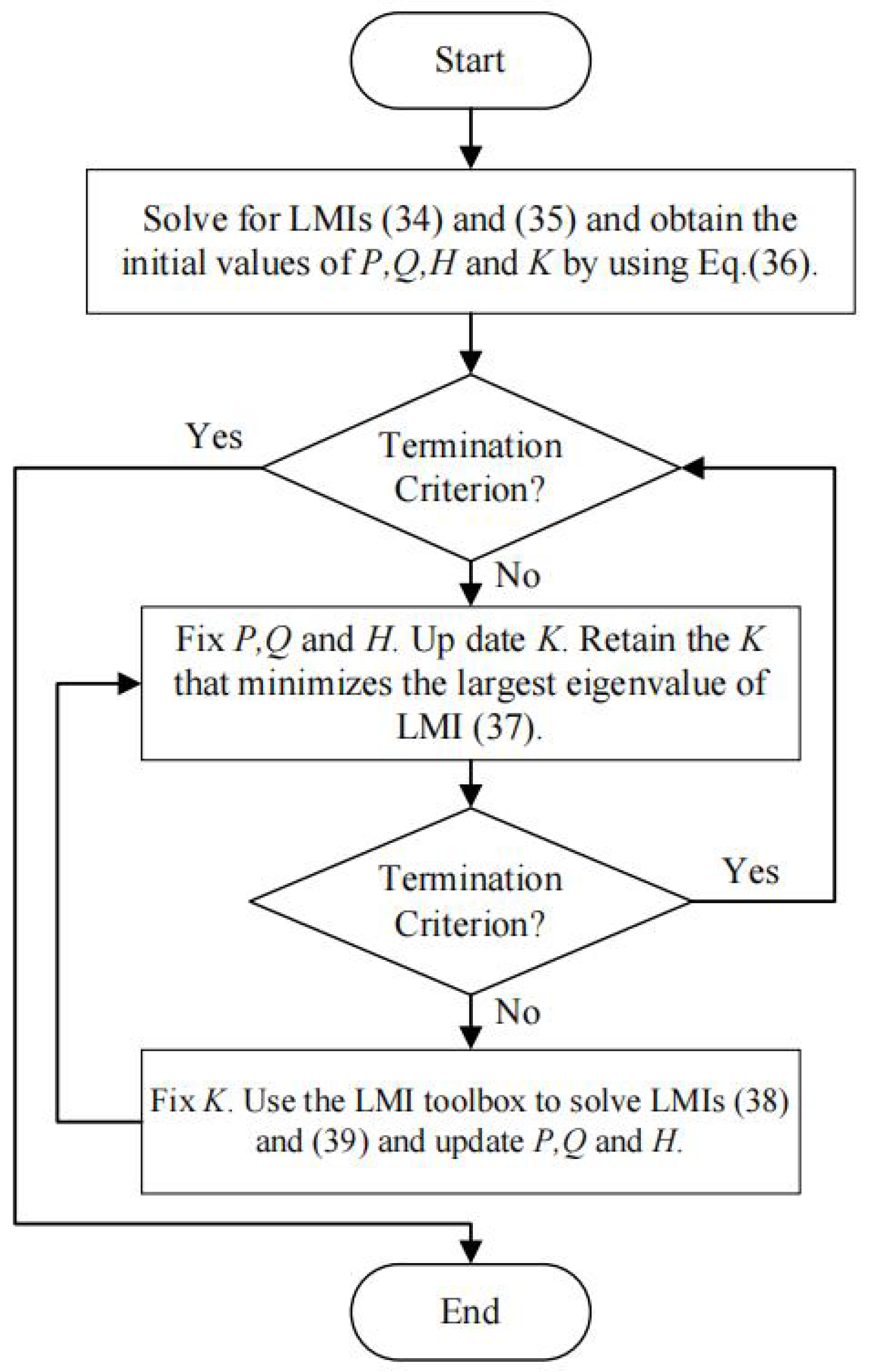
Solve the initial LMI system	Use MATLAB LMI toolbox to solve the LMIs (34)–(36) to obtain the initial values $P_1,Q_1,H_1$, and $K_1$.
Inner iteration: update K	With P, Q, and H fixed, the MATLAB LMI toolbox is used to solve LMI (38) to update the initial value of K in the internal iteration. Then, update K using increasing step size $I_{u_k}$ or the decreasing step size $I_{d_k}$ for, at most, $N_k$ iterations. Evaluate eigenvalues of (37) to check feasibility.
Step size adjustment	For the K obtained after each internal iteration, if the maximum positive eigenvalue of (37) increases, reduce the step size to half of the original.
	Then, if the maximum positive eigenvalue of (37) still increases, switch the step size, i.e., switch the increasing step size to a decreasing step size or switch the decreasing step size to an increasing step size.
	If the maximum positive eigenvalue of (37) decreases, increase the step size to twice the original.
	Then, if the maximum positive eigenvalue of (37) still decreases, continue to increase the step size.
Update P, Q, and H	With K fixed, use MATLAB LMI toolbox to solve the LMI (39) and update P, Q, and H.
Termination	If the eigenvalues of LMI (37) are all negative, return optimal K. If not, return the best K obtained and the corresponding eigenvalue condition.

.

Remark 7. 

The proposed algorithm solves an LMI problem in each iteration, with computational complexity primarily determined by the dimensions of the matrix variables. It involves a two-level iterative process: the outer loop updates $P,Q,$ and H, while the inner loop adjusts the feedback gain K via step size control. The overall complexity is approximately $O(N·N_k)$. For high-dimensional systems or slow convergence, the computational burden increases significantly. Numerical stability may be affected by matrix inversion and eigenvalue computations, especially near-singular matrices or eigenvalues close to zero. Proper step size selection and termination criteria are essential. Robustness can be enhanced by introducing constraints, such as bounding the spectral radius of P.

4. Numerical Examples

Numerical examples are provided to verify the results presented in Section 3. These examples serve to confirm the theoretical findings and demonstrate their validity under various conditions.

Example 1. 

Set the parameters of System (2) as $\alpha =0.6$ and

$$E=\left[\begin{array}{ccc}4& 2& 6\\ 7& 0& 4\\ 7& 0& 4\end{array}\right],A=\left[\begin{array}{ccc}4& -2& -3\\ -3& -1& -6\\ -3& 4& 1\end{array}\right].$$

It has been verified that $det(\lambda E-A)=-32{\lambda }^2-43\lambda -95$, indicating that the system in Example 1 is regular. The degree of $det(\lambda E-A)$, given by $deg(det(\lambda E-A\left)\right)=\mathrm{rank}\left(E\right)=2$, implies that the system in Example 1 is impulse-free. The roots of the characteristic polynomial $det(\lambda E-A)=0$ are $-0.6719\pm 1.5866\mathrm{j}$. All roots satisfy the stability condition $\left|arg\left(\mathrm{spec}\left(E,A\right)\right)\right|>\alpha {\displaystyle \frac{\pi }{2}}$, which confirms the stability of the system in Example 1. Therefore, the system in Example 1 is admissible. Set $S={\left[\begin{array}{ccc}0& 1& -1\end{array}\right]}^T$. Solving the LMIs (6) and (7) yields the following feasible solutions:

$$\begin{array}{c}\hfill P=\left[\begin{array}{ccc}20.5820& -6.7861& -6.7861\\ -6.7861& -185.6321& 192.5336\\ -6.7861& 192.5336& -185.6321\end{array}\right],Q=\left[\begin{array}{ccc}0& 9.7232& -10.2875\\ -9.7232& 0& 17.2646\\ 10.2875& -17.2646& 0\end{array}\right].\end{array}$$

Solving the LMIs (24) and (25) yields the following feasible solution:

$$X=\left[\begin{array}{ccc}10.2910& 1.4686& -8.5368\\ -8.2546& -92.8160& 104.8991\\ 1.7507& 87.6345& -92.8160\end{array}\right].$$

The feasible solutions obtained by solving the LMIs in (26) and (27) are as follows:

$$\begin{array}{cc}& P=\left[\begin{array}{ccc}70.8939& -18.6547& -18.6547\\ -18.6547& -102.4241& 117.6885\\ -18.6547& 117.6885& -102.4241\end{array}\right],Q=\left[\begin{array}{ccc}0& 34.3500& -37.3959\\ -34.3500& 0& 62.4540\\ 37.3959& -62.4540& 0\end{array}\right],\hfill \\ & H=\left[\begin{array}{ccc}40.3752& 10.1722& 71.5487\end{array}\right].\hfill \end{array}$$

The state responses of the system in Example 1 are shown in Figure 2, which shows that the system is admissible and its state tends to zero.

As a comparison, for the parameters of the singular FOS in Example 1, the feasible solution is solved using the method shown in Theorem 2 in [31]. It is not possible to define complex variables directly in MATLAB, so it is necessary to use two real variables to define the complex variable X in programming, which increases the programming difficulty. In addition, set $S={\left[\begin{array}{ccc}-0.2615& -0.8498& 0.4576\end{array}\right]}^T$. Solving the LMIs of Theorem 2 in [31] yields feasible solutions as follows:

$$\begin{array}{cc}& X={10}^3\left[\begin{array}{ccc}2.3477& 1.3031& -1.7284\\ 1.3031& 6.6862& -2.8081\\ -1.7284& -2.8081& 2.3671\end{array}\right]+{10}^3\left[\begin{array}{ccc}0& 2.2879& -0.4008\\ -2.2879& 0& 2.2149\\ 0.4008& -2.2149& 0\end{array}\right]\mathrm{j},\hfill \\ & Y={10}^3{\left[\begin{array}{ccc}0.7315& 7.4587& 4.0505\end{array}\right]}^T.\hfill \end{array}$$

It can be seen that the order of magnitude of the feasible solutions obtained is bad, while the order of magnitude of the solutions obtained using our approach is valid.

Example 2. 

Set the parameters of System (2) as $\alpha =0.5$, and

$$E=\left[\begin{array}{ccc}-5& -22& -25\\ 4& -11& -2\\ 7& -16& -1\end{array}\right],A=\left[\begin{array}{ccc}5& -4& -2\\ -2& 2& -1\\ -4& 3& -2\end{array}\right],B=\left[\begin{array}{c}3\\ 2\\ 4\end{array}\right].$$

Similar to the calculations in Example 1, it is verified that the system in Example 2 is regular and impulse-free when $\alpha =0.5$. However, the system is unstable, indicating that it is not admissible. Set $S={\left[\begin{array}{ccc}13& -234& 143\end{array}\right]}^T,N=100,N_k=50,I_k=0.01,I_{u_k}=0.02,I_{d_k}=-0.04,$ and the spectral radius of the matrix P is ${10}^4$. According to the BBA shown in Figure 1, the feasible solutions are obtained as:

$$\begin{array}{cc}& P={10}^4\left[\begin{array}{ccc}-5.6471& -2.7100& 3.5317\\ -2.7100& -1.2764& 1.6589\\ 3.5317& 1.6589& -2.1427\end{array}\right],Q=\left[\begin{array}{ccc}0& -254.0788& 622.7066\\ 254.0788& 0& 132.6209\\ -622.7066& -132.6209& 0\end{array}\right],\hfill \\ & H=\left[\begin{array}{ccc}-35.5814& -8.9278& -13.2592\end{array}\right],K=\left[\begin{array}{ccc}19.1699& -99.0303& -164.5462\end{array}\right].\hfill \end{array}$$

The proposed BBA was implemented and executed in MATLAB R2024a on a laptop equipped with an Intel(R) Core(TM) i5-8250U CPU @ 1.60GHz (1.80GHz turbo). The execution time for a single run of the algorithm was approximately 0.0289 s, indicating that the method is computationally efficient and suitable for real-time or iterative design applications in low-dimensional systems. As shown in Figure 3, although the open-loop singular system is unstable, the state feedback controller (29) can be employed to stabilize the closed-loop system.

Remark 8. 

Example 2 can be solved for admissibility and stabilization singular FOSs of an order between $(0,1)$ via strict LMI frameworks. Referring to

Table 2. Comparison of the proposed approaches with existing results for FOSs.

Ref.	System Type	Fractional-Order Field	Variables	No Equality Constraints	No Bilinear Problem
Theorem 3 in [31]	Singular FOSs	$\alpha \in (0,1)$	6	✓	×
Theorem 2 in [32]	Singular FOSs	$\alpha \in [1,2)$	5	✓	×
Theorem 1 in [29]	Singular FOSs	$\alpha \in [1,2)$	4	×	✓
Theorem 1 in [28]	FOSs	$\alpha \in (0,1)$	4	✓	✓
Our Theorems 1 and 2	Singular FOSs	$\alpha \in (0,1)$	2/3	✓	✓
Our Corollary 1	Singular FOSs	$\alpha \in (0,1)$	1	✓	✓
Our Theorem 3	Singular FOSs	$\alpha \in (0,1)$	3	✓	×

, our approaches involve fewer real decision variables and remove the equality constraints, which makes it easy to solve for the decision variables. Overall, from the comparison in Table 2, our results outperform the existing ones.

Example 3. 

Consider electrical circuit from [5] shown in Figure 4. It includes resistor R; capacitors $C_1,C_2,C_3$ in the supercondensator; and source voltages $e_1$ and $e_2$, where the relationship between current and charge in a capacitor can be modeled succinctly and accurately using a fractional-order system. Specifically, let the current $i_C\left(t\right)$ in the supercondensator with the capacity C be the α order derivative of its charge $q\left(t\right)$

$$i_C\left(t\right)={\displaystyle \frac{d^{\alpha }q\left(t\right)}{d{t}^{\alpha }}}.$$

Taking into account that $q\left(t\right)=C{u}_C\left(t\right)$, we obtain

$$i_C\left(t\right)=C{\displaystyle \frac{d^{\alpha }{u}_C\left(t\right)}{d{t}^{\alpha }}}.$$

The electrical circuit the equations are as follows:

$$\left[\begin{array}{ccc}R{C}_1& 0& 0\\ C_1& C_2& -C_3\\ 0& 0& 0\end{array}\right]{\displaystyle \frac{d^{\alpha }}{d{t}^{\alpha }}}\left[\begin{array}{c}{u}_1\\ u_2\\ u_3\end{array}\right]=\left[\begin{array}{ccc}-1& 0& -1\\ 0& 0& 0\\ 0& -1& -1\end{array}\right]\left[\begin{array}{c}{u}_1\\ u_2\\ u_3\end{array}\right]+\left[\begin{array}{cc}1& 0\\ 0& 0\\ 0& 1\end{array}\right]\left[\begin{array}{c}{e}_1\\ e_2\end{array}\right].$$

(40)

Let $\alpha =0.78$ and $R=C_1=C_2=C_3=1$; the system can be readily verified to be regular, impulse-free, and unstable. Set $S={\left[\begin{array}{ccc}0& 0& 1\end{array}\right]}^T,N=100,N_k=50,I_k=0.01,I_{u_k}=0.01,$$I_{d_k}=-0.02,$ and the spectral radius of the matrix P is ${10}^8$. According to the BBA shown in Figure 1, the feasible solutions are obtained as:

$$\begin{array}{cc}& P={10}^8\left[\begin{array}{ccc}0.0670& -0.0035& -0.0033\\ -0.0035& -2.1484& -2.2187\\ -0.0033& -2.2187& -2.1555\end{array}\right],Q={10}^7\left[\begin{array}{ccc}0& 2.5118& 2.5102\\ -2.5118& 0& -2.4945\\ -2.5102& 2.4945& 0\end{array}\right],\hfill \\ & H={10}^8\left[\begin{array}{ccc}1.6863& -0.0475& -7.3304\end{array}\right],K=\left[\begin{array}{ccc}-117.9231& 120.3295& 1.4042\\ 120.0179& -120.7647& -0.7122\end{array}\right].\hfill \end{array}$$

Using the $tic$ and $toc$ commands, we know that the program runs in 0.0311 s. The running time is also very short for similar reasons as in Example 2. Involving the gain matrix K obtained using the BBA shown in Figure 1, the state responses of the closed-loop system in Example 3 are shown in Figure 5. It is clear that while the open-loop singular system is unstable, the closed-loop singular system is admissible.

5. Conclusions

In this paper, we study the admissibility criterion and stabilization criterion for fractional-order singular FOSs in a class of intervals $(0,1)$. The successful generalization of the strict LMI stability criterion for IOS to FOSs has never been reported before, enriching the results of the admissibility criteria. The improved criterion that involved only one matrix variable reflects the admissibility of singular FOSs more essentially and simplifies the programming. The designed BBA effectively solves the bilinear constraints that are difficult to solve for feasible solutions with the MATLAB LMI toolbox and facilitates the synthesis of state feedback controllers. For the singular FOSs in this paper, our future work is to propose a robust stabilization criterion based on the method in this paper.

References

- Lim, Y.; Oh, M.; Ahn, H. Stability and stabilization of fractional-order linear systems subject to input saturation. IEEE Trans. Autom. Control 2013, 58, 1062–1067. [Google Scholar] [CrossRef]
- Zhang, X.F.; Liu, R.; Ren, J.X.; Cui, Q.L. Adaptive fractional image enhancement algorithm based on rough set and particle swarm optimization. Fractal Fract. 2022, 6, 100. [Google Scholar] [CrossRef]
- Sabatier, J.; Moze, M.; Farges, C. On stability of fractional order systems. In Proceedings of the Third IFAC Workshop on Fractional Differentiation and Its Applications FDA’08, Ankara, Turkey, 5–7 November 2008. [Google Scholar]
- Zhang, X.F.; Lin, C.; Chen, Y.Q.; Boutat, D. A unified framework of stability theorems for LTI fractional order systems with 0 < α < 2. IEEE Trans. Circuits Syst. II Express Briefs 2020, 67, 3237–3241. [Google Scholar]
- Zhang, X.F.; Chen, Y.Q. Admissibility and robust stabilization of continuous linear singular fractional order systems with the fractional order α: The 0 < α < 1 case. ISA Trans. 2018, 82, 42–50. [Google Scholar] [CrossRef] [PubMed]
- Wang, L.; Zeng, X.M.; Yang, H.M.; Lv, X.D.; Guo, F.X.; Shi, Y.; Hanif, A. Investigation and application of fractal theory in cement-based materials: A review. Fractal Fract. 2021, 5, 247. [Google Scholar] [CrossRef]
- Zhang, J.-X.; Zhang, X.F.; Boutat, D.; Liu, D.-Y. Fractional-order complex systems: Advanced control, intelligent estimation and reinforcement learning image-processing algorithms. Fractal Fract. 2025, 9, 67. [Google Scholar] [CrossRef]
- Huang, L.L.; Wu, G.C.; Baleanu, D.; Wang, H.Y. Discrete fractional calculus for interval-valued systems. Fuzzy Sets Syst. 2021, 404, 141–158. [Google Scholar] [CrossRef]
- Gong, P.; Lan, W.; Han, Q.L. Robust adaptive fault-tolerant consensus control for uncertain nonlinear fractional-order multi-agent systems with directed topologies. Automatica 2020, 117, 109011. [Google Scholar] [CrossRef]
- Wang, X.Y.; Zhang, X.F.; Pedrycz, W.; Yang, S.-H.; Boutat, D. Consensus of T-S fuzzy fractional-order, singular perturbation, multi-agent systems. Fractal Fract. 2024, 8, 523. [Google Scholar] [CrossRef]
- Guo, Y.; Lin, C. The disturbance rejection control of fractional-order system. Math. Method. Appl. Sci. 2025, 48, 11559–12614. [Google Scholar] [CrossRef]
- Zhang, J.-X.; Ding, J.L.; Chai, T.Y. Fault-tolerant prescribed performance control of wheeled mobile robots: A mixed-gain adaption approach. IEEE Trans. Autom. Control 2024, 69, 5500–5507. [Google Scholar] [CrossRef]
- Zhang, J.-X.; Xu, K.D.; Wang, Q.-G. Prescribed performance tracking control of time-delay nonlinear systems with output constraints. IEEE/CAA J. Autom. Sin. 2024, 11, 1557–1565. [Google Scholar] [CrossRef]
- Zhang, J.-X.; Ding, J.L.; Chai, T.Y. Cyclic performance monitoring-based fault-tolerant funnel control of unknown nonlinear systems with actuator failures. IEEE Trans. Autom. Control 2025. early access. [Google Scholar] [CrossRef]
- Zhang, J.-X.; Cui, E.-Y.; Shi, P. Low-complexity high-performance control of unknown block-triangular MIMO nonlinear systems. IEEE Trans. Ind. Electron. 2024, 72, 7515–7523. [Google Scholar] [CrossRef]
- Zhang, J.-X.; Yang, G.-H. Low-complexity tracking control of strict-feedback systems with unknown control directions. IEEE Trans. Autom. Control 2019, 64, 5175–5182. [Google Scholar] [CrossRef]
- Zhang, J.-X.; Liu, Y.-Q.; Chai, T.Y. Singularity-free low-complexity fault-tolerant prescribed performance control for spacecraft attitude stabilization. IEEE Trans. Autom. Sci. Eng. 2025, 22, 15408–15419. [Google Scholar] [CrossRef]
- Wu, J.L.; Yung, C.F. A new generalized bounded real lemma for continuous-time descriptor systems. Asian J. Control 2022, 24, 2729–2737. [Google Scholar] [CrossRef]
- Feng, Z.; Shi, P. Two equivalent sets: Application to singular systems. Automatica 2017, 77, 198–205. [Google Scholar] [CrossRef]
- Matignon, D. Stability result on fractional differential equations with applications to control processing. Comput. Eng. Syst. Appl. 1996, 2, 963–968. [Google Scholar]
- Amini, A.; Azarbahram, A.; Sojoodi, M. H∞ consensus of nonlinear multi-agent systems using dynamic output feedback controller: An LMI approach. Nonlinear Dyn. 2016, 85, 1865–1886. [Google Scholar] [CrossRef]
- El-Khazali, R.; Momani, S. Stability analysis of composite fractional systems. Int. J. Appl. Math. 2003, 12, 73–85. [Google Scholar]
- Tavazoei, M.; Haeri, M. A note on the stability of fractional order systems. Math. Comput. Simul. 2009, 79, 1566–1576. [Google Scholar] [CrossRef]
- Ahn, H.; Chen, Y.Q. Necessary and sufficient stability condition of fractional-order interval linear systems. Automatica 2008, 44, 2985–2988. [Google Scholar] [CrossRef]
- Sabatier, J.; Moze, M.; Farges, C. LMI stability conditions for fractional order systems. Comput. Math. Appl. 2010, 59, 1594–1609. [Google Scholar] [CrossRef]
- Farges, C.; Moze, M.; Sabatier, J. Pseudo-state feedback stabilization of commensurate fractional order systems. Automatica 2010, 46, 1730–1734. [Google Scholar] [CrossRef]
- Jiao, Z.; Zhong, Y. Robust stability for fractional-order systems with structured and unstructured uncertainties. Comput. Math. Appl. 2012, 3258–3266. [Google Scholar] [CrossRef]
- Lu, J.G.; Chen, Y.Q. Robust stability and stabilization of fractional-order interval systems with the fractional order α: The 0 < α < 1 Case. IEEE Trans. Autom. Control 2009, 152–158. [Google Scholar]
- Marir, S.; Chadli, M.; Basin, M. Necessary and sufficient admissibility conditions of dynamic output feedback for singular linear fractional-order systems. Asian J. Control 2023, 25, 2439–2450. [Google Scholar] [CrossRef]
- Liu, Y.C.; Cui, L.; Duan, D.P. Dynamic output feedback stabilization of singular fractional-order systems. Math. Probl. Eng. 2016, 9694780. [Google Scholar] [CrossRef]
- Marir, S.; Chadli, M.; Bouagada, D. A novel approach of admissibility for singular linear continuous-time fractional-order systems. Int. J. Control Autom. Syst. 2017, 15, 959–964. [Google Scholar] [CrossRef]
- Marir, S.; Chadli, M. Robust admissibility and stabilization of uncertain singular fractional-order linear time-invariant systems. IEEE/CAA J. Autom. Sin. 2019, 6, 685–692. [Google Scholar] [CrossRef]
- Ji, Y.; Qiu, J.Q. Stabilization of fractional-order singular uncertain systems. ISA Trans. 2015, 56, 53–643. [Google Scholar] [CrossRef] [PubMed]
- N’Doye, I.; Darouach, M.; Zasadzinski, M.; Radhy, N. Robust stabilization of uncertain descriptor fractional-order systems. Automatica 2013, 49, 1907–1913. [Google Scholar] [CrossRef]
- Wei, Y.H.; Tse, P.W.; Yao, Z.; Wang, Y. The output feedback control synthesis for a class of singular fractional order systems. ISA Trans. 2017, 69, 1–9. [Google Scholar] [CrossRef]
- Shen, J.; Lam, J. State feedback H∞ control of commensurate fractional-order systems. Int. J. Syst. Sci. 2014, 45, 363–372. [Google Scholar] [CrossRef]
- Marir, S.; Chadli, M.; Basin, M. Bounded real lemma for singular linear continuous-time fractional-order systems. Automatica 2022, 135, 109962. [Google Scholar] [CrossRef]
- Di, Y.; Zhang, J.-X.; Zhang, X.F. Robust stabilization of descriptor fractional-order interval systems with uncertain derivative matrices. Appl. Math. Comput. 2023, 453, 128076. [Google Scholar] [CrossRef]
- Zhang, L.X.; Zhang, J.-X.; Zhang, X.F. Generalized criteria for admissibility of singular fractional order systems. Fractal Fract. 2023, 7, 363. [Google Scholar] [CrossRef]