Inverse Problem for a Time-Dependent Source in Distributed-Order Time-Space Fractional Diffusion Equations

Abstract

This paper investigates the problem of identifying a time-dependent source term in distributed-order time-space fractional diffusion equations (FDEs) based on boundary observation data. Firstly, the existence, uniqueness, and regularity of the solution to the direct problem are proved. Using the regularity of the solution and a Gronwall inequality with a weakly singular kernel, the uniqueness and stability estimates of the solution to the inverse problem are obtained. Subsequently, the inverse source problem is transformed into a minimization problem of a functional using the Tikhonov regularization method, and an approximate solution is obtained by the conjugate gradient method. Numerical experiments confirm that the method provides both accurate and robust results.

1. Introduction

In recent decades, researchers in the field of physics have discovered an anomalous super-slow diffusion process characterized by logarithmic growth in mean square displacement [1,2,3]. These processes find widespread applications in various fields such as physics, polymer science, and particle dynamics. Compared to certain anomalous diffusion forms described by fractional-order models, these processes exhibit higher complexity. The traditional framework of fractional diffusion models is insufficient to fully describe the phenomenon of super-slow diffusion. To better characterize this phenomenon, the mathematical community has developed distributed-order FDEs as a more comprehensive modeling framework. Extensive research has been conducted on initial-boundary value problems (IBVPs) for distributed-order FDEs, with significant contributions made in theoretical analysis, numerical methods, and applications (see references [4,5,6,7,8]). However, in practical applications, we often encounter situations where certain critical parameters, such as boundary conditions, initial values, diffusion coefficients, or source terms are unavailable. These limitations necessitate the reconstruction of unknown quantities using supplementary measurement data. Consequently, this results in the occurrence of inverse problems associated with fractional differential equations. This inverse problem framework has become increasingly important in various scientific and engineering fields where complete system information is inaccessible.

The inverse source problem continues to attract significant attention within the scientific community, owing to its wide-ranging applications in areas such as medical imaging, geophysical exploration, and other applied sciences. For classical elliptic and parabolic partial differential equations, substantial progress has been achieved in source identification, giving rise to a comprehensive and well-established body of research. In contrast, the study of inverse source problems for FDEs is comparatively less developed and remains at an early stage. To date, most research efforts have focused on time FDEs, with notable results and advancements documented in works such as [9,10,11,12]. However, there remains much to explore in this area, including both theoretical challenges and practical applications.

For the inverse problem of distributed-order FDEs, several results have already been achieved, for instance, determining the weight function of the distributed derivative [13,14,15,16], the backward problem [17,18], and the inverse potential problem [19,20].

Regarding the inverse source problem for distributed-order FDEs, Zhang and Liu [21] addressed the challenge of recovering time-dependent internal sources from nonrestrictive integral observations. Sun and Liu [22] investigated the solvability of the time-distributed order equation for an inverse problem with a time-dependent source term, developed a gradient-type algorithm, and presented supporting numerical results. Hai [23] examined the time-distributed order diffusion equation with a spatially dependent source term on the Hilbert scale and proposed a general regularization technique based on filtering methods.

We address the DTSFDE presented in the form below

$${\partial }_{0^{+}}^{(\mu )}u(x,t)=-{(-\Delta )}^{{\displaystyle \frac{\beta }{2}}}u(x,t)+p(t)f(x),(x,t)\in \Omega \times (0,T],$$

(1)

where $\Omega \subset R^d$ and $d=1,2,\dots$, $T>0$ is the final time, ${\partial }_{0^{+}}^{(\mu )}u(x,t)$ is the distributed order derivative operator defined by

$${\partial }_{0^{+}}^{(\mu )}u(x,t)={\int }_0^1\mu (\alpha ){\partial }_{0^{+}}^{\alpha }u(x,t)d\alpha ,t\in (0,T],0<\alpha <1,$$

with a weight function $\mu (\alpha )\ge 0$ satisfying $\mu \in L^1(0,1)$ and ${\int }_0^1\mu (\alpha )d\alpha =c_0>0$ [24], and ${\partial }_{0^{+}}^{\alpha }u$ is the Caputo fractional derivative

$${\partial }_{0^{+}}^{\alpha }u(x,t)={\displaystyle \frac{1}{\Gamma (1-\alpha )}}{\int }_0^t{\displaystyle \frac{\partial u(x,s)}{\partial s}}{\displaystyle \frac{\mathrm{d}s}{{(t-s)}^{\alpha }}},t\in (0,T],0<\alpha <1,$$

where $\Gamma (·)$ is the Gamma function.

The fractional Laplacian operator ${(-\Delta )}^{{\displaystyle \frac{\beta }{2}}}$ is defined for $\beta (1<\beta \le 2)$ with the spectral decomposition for the Laplace operator $-\Delta$ [25]. The definition is summarized in Definition 1 in Section 2.

The unknown function u is assumed to satisfy the following initial and boundary conditions:

$$\begin{array}{c}\hfill \left\{\begin{array}{c}u(x,0)=a(x),x\in \overline{\Omega },\hfill \\ {\displaystyle \frac{\partial u}{\partial n}}(x,t)=0,(x,t)\in \partial \Omega \times (0,T].\hfill \end{array}\right.\end{array}$$

(2)

If the source term and initial values are known, Equations (1) and (2) become a forward problem, while the inverse problem is to infer the time term $p(t)$ from the following additional data in the problem ((1) and (2)):

$$u(x,t)=G(x,t),in\Gamma ,$$

(3)

where $\Gamma$ is a part of the $\partial \Omega$.

Based on the information available to us, the identification of the source term in a distributed-order time-space FDE is a relatively recent research topic with substantial scientific and practical significance. Currently, few studies—either domestically or internationally—have addressed this issue, which highlights the novelty and importance of the problem investigated in this work.

2. Preliminaries

In the following discussion, we utilize right-sided distributed-order derivatives, defined as

$${\partial }_{T^{-}}^{(\mu )}v(t)={\int }_0^1\mu (\alpha ){\partial }_{T^{-}}^{\alpha }v(t))d\alpha ,\alpha \in (0,1),$$

(4)

where ${\partial }_{T^{-}}^{\alpha }v(t)$ is the right-sided Caputo fractional derivative given by

$${\partial }_{T^{-}}^{\alpha }v(t)=-{\displaystyle \frac{1}{\Gamma (1-\alpha )}}{\int }_t^{T}v(t){(s-t)}^{-\alpha }ds.$$

(5)

Additionally, for $\alpha \in (0,1)$, the operators $I_{0^{+}}^{\alpha }v(t)$ and $I_{T^{-}}^{\alpha }v(t)$ denote the left- and right-sided Riemann–Liouville fractional integrals, respectively:

$$\begin{array}{c}\hfill \left\{\begin{array}{c}{I}_{0^{+}}^{\alpha }v(t)={\displaystyle \frac{1}{\Gamma (\alpha )}}{\int }_0^{t}v(s){(t-s)}^{\alpha -1}ds,\hfill \\ I_{T^{-}}^{\alpha }v(t)={\displaystyle \frac{1}{\Gamma (\alpha )}}{\int }_t^{T}v(s){(s-t)}^{\alpha -1}ds.\hfill \end{array}\right.\end{array}$$

(6)

Next, we present the spectral decomposition definition of the fractional Laplacian operator (for more information on the properties and physical significance of the fractional Laplacian operator $-{\Delta }^{{\displaystyle \frac{\beta }{2}}}$, please refer to reference [25]).

Definition 1 

(see [26,27,28]). Let ${\overline{\lambda }}_n$ and ${\psi }_n$ denote the eigenvalues and corresponding eigenfunctions of the negative Laplacian, satisfying

$$\left\{\begin{array}{c}-\Delta {\psi }_n={\overline{\lambda }}_n{\psi }_n,in\Omega ,\\ {\displaystyle \frac{\partial {\psi }_n}{\partial n}}=0,on\partial \Omega ,\end{array}\right.$$

with the eigenvalues fulfilling $0={\overline{\lambda }}_0<{\overline{\lambda }}_1\le \dots \le {\overline{\lambda }}_n\le \dots$.

For $1<\beta \le 2$, we define the Hilbert space

$$D({(-\Delta +1)}^{{\displaystyle \frac{\beta }{2}}})=\{v=\sum _{n=0}^{\infty }{a}_n{\psi }_n\in L^2{(\Omega ):\parallel v\parallel }_{D({(-\Delta +1)}^{{\displaystyle \frac{\beta }{2}}})}^2=\sum _{n=0}^{\infty }{a}_n^2{({\overline{\lambda }}_n+1)}^{\beta }<\infty \}.$$

For any $v\in D({(-\Delta +1)}^{{\displaystyle \frac{\beta }{2}}})$, the fractional Laplacian operators are defined as

$${(-\Delta )}^{{\displaystyle \frac{\beta }{2}}}v=\sum _{n=0}^{\infty }{a}_n{\overline{\lambda }}_n^{{\displaystyle \frac{\beta }{2}}}{\psi }_n,{(-\Delta +1)}^{{\displaystyle \frac{\beta }{2}}}v=\sum _{n=0}^{\infty }{a}_n{({\overline{\lambda }}_n+1)}^{{\displaystyle \frac{\beta }{2}}}{\psi }_n,$$

which are bounded linear operators mapping $D({(-\Delta +1)}^{{\displaystyle \frac{\beta }{2}}})$ into $L_2(\Omega )$. Furthermore, the following norm equivalence holds:

$${\parallel v\parallel }_{D({(-\Delta +1)}^{{\displaystyle \frac{\beta }{2}}})}={|{(-\Delta +1)}^{{\displaystyle \frac{\beta }{2}}}v|}_{L_2(\Omega )}.$$

For simplicity, throughout the remainder of the paper, we denote ${\lambda }_n={\overline{\lambda }}_n^{\beta /2}$.

To facilitate subsequent analysis, we present several definitions, properties, and lemmas from fractional calculus.

Lemma 1 

([29]). Suppose ${\psi }_n(x)$ is the eigenfunction of $(-\Delta )$ associated with the eigenvalue ${\overline{\lambda }}_n$ in Ω, and let g denote a sufficiently smooth function. Then,

$$({\psi }_n,{(-\Delta )}^{{\displaystyle \frac{\beta }{2}}}g)={\overline{\lambda }}_n^{{\displaystyle \frac{\beta }{2}}-1}{\int }_{\partial \Omega }\left({\displaystyle \frac{\partial \phi }{\partial n}}g(x)-{\psi }_n(x){\displaystyle \frac{\partial g}{\partial n}}\right)dS+({(-\Delta )}^{{\displaystyle \frac{\beta }{2}}}{\psi }_n,g).$$

Lemma 2 

([30]). Assume $f_1(t),f_2(t)\in AC[0,T]$, then

$${\int }_0^T({\partial }_{0^{+}}^{(\mu )}{f}_1)(t)f_2(t)dt-{\int }_0^T{f}_1(t)({\partial }_{T^{-}}^{(\mu )}{f}_2)(t)dt=-f_1(0)(H_{T^{-}}^{(\mu )}{f}_2)(0)+(H_{0^{+}}^{(\mu )}{f}_1)(T)f_2(T),$$

(7)

where

$$(H_{0^{+}}^{(\mu )}{f}_1)(t)={\int }_0^1\mu (\alpha )I_{0^{+}}^{1-\alpha }{f}_1(t)d\alpha ,(H_{T^{-}}^{(\mu )}{f}_2)(t)={\int }_0^1\mu (\alpha )I_{T^{-}}^{1-\alpha }{f}_2(t)d\alpha .$$

(8)

Lemma 3. 

([31]). Let $0<\alpha <1$ and $f(t)\in C^1(0,T)$, then

$$L({\partial }_{0+}^{\alpha }f)(s)=s^{\alpha }(Lf)(s)-s^{\alpha -1}f(0).$$

(9)

To facilitate the presentation of the solution to Equation (1), we introduce the following distributed-order ordinary differential equation:

$$\begin{array}{c}\hfill \left\{\begin{array}{c}{\partial }_{0^{+}}^{(\mu )}{\omega }_n(t)=-{\lambda }_n{\omega }_n(t),t\in (0,T]\hfill \\ {\omega }_n(0)=1.\hfill \end{array}\right.\end{array}$$

(10)

The uniqueness of the solution to the above equation can be found in [15]. By [22], ${\omega }_n(t)$ has the following properties:

Lemma 4. 

If $\mu \not\equiv 0$ and $\mu (0)\ne 0$, then the following conclusion holds:

1. 

For $n\in N^{+}$, let ${\omega }_n(t)\in C[0,T)\cap C^{\infty }(0,T)$ be a completely monotonic function, that is ${(-1)}^n{\displaystyle \frac{d^n}{d{t}^n}}{\omega }_n(t)\ge 0,$

2. 

$0\le {\omega }_n(t)\le 1$ for $t\in [0,T]$.

3. 

If $t^{1-\xi }{\displaystyle \frac{d}{dt}}{\omega }_n(t)$ is continuous and bounded on the interval $[0,T]$, then it holds that

$$0\le -{\displaystyle \frac{d}{dt}}{\omega }_n(t)\le C{\lambda }_n{t}^{\xi -1},\xi \in \left(0,{\displaystyle \frac{1}{2}}\right).$$

Lemma 5 

(see [15]). Defining operators $K_{0^{+}}^{(\mu )}{\omega }_n$,

$$K_{0^{+}}^{(\mu )}{\omega }_n(t)={\int }_0^t\chi (t-\tau ){\omega }_n(\tau )d\tau ,where\chi (t)={\displaystyle \frac{1}{2\pi i}}{\int }_{\gamma -i\infty }^{\gamma +i\infty }{\displaystyle \frac{e^{st}}{{\int }_0^1\mu (\alpha ){\mathrm{s}}^{\alpha }d\alpha }}ds,$$

then the following conclusions hold:

1.

$\chi (t)\in C^{\infty }(0,\infty ),$

2.

$(K_{0+}^{(\mu )}{\partial }_{0+}^{(\mu )}){\omega }_n(t)={\omega }_n(t)-{\omega }_n(0)$,

3.

$({\partial }_{0+}^{(\mu )}{K}_{0+}^{(\mu )}){\omega }_n(t)={\omega }_n(t),$ for ${\omega }_n\in C^{\infty }(0,T)$.

Lemma 6. 

Suppose $p(t)\in C^1[0,T]$, ${\lambda }_n\ge 0$, define $r_0(t)$, $r_n(t)$ as follows:

$$\begin{array}{cc}\hfill r_0(t)=& {\int }_0^t{\displaystyle \frac{dp(\tau )}{d\tau }}{K}_{0^{+}}^{(\mu )}{\omega }_0(t-\tau )d\tau +p(0)K_{0^{+}}^{(\mu )}{\omega }_0(t),\hfill \\ \hfill r_n(t)=& {\displaystyle \frac{1}{{\lambda }_n}}{\int }_0^{t}p(\tau ){\displaystyle \frac{d}{d\tau }}{\omega }_n(t-\tau )d\tau ,n=1,2,\dots ,\hfill \end{array}$$

then $r_0(t),r_n(t)\in C[0,T]$ and

$$\begin{array}{cc}\hfill |r_0(t)|\le & {C(T\parallel p\parallel }_{C^1[0,T]}+{1)\parallel \chi \parallel }_{L^1(0,T]},\hfill \\ \hfill |r_n(t)|\le & {C\parallel p\parallel }_{C^1[0,T]},n=1,2,\dots .\hfill \end{array}$$

Proof.  

(1) When ${\lambda }_0=0$, it is obvious that ${\omega }_0(t)=1$, so we can obtain

$${\int }_0^t{\displaystyle \frac{dp(\tau )}{d\tau }}{K}_{0^{+}}^{(\mu )}{\omega }_0(t-\tau )d\tau ={\displaystyle \frac{dp(t)}{dt}}\ast K_{0^{+}}^{(\mu )}{\omega }_0(t)$$

and

$$K_{0^{+}}^{(\mu )}{\omega }_0(t)={\int }_0^t\chi (t-\tau ){\omega }_0(\tau )d\tau =\chi (t)\ast {\omega }_0(t)$$

Given conditions of $p\in C^1[0,T]$ and $K_{0^{+}}^{(\mu )}{\omega }_0(t)\in L^1(0,T]$, we can directly infer using Young’s inequality that $r_0(t)\in C[0,T]$ (refer to [32], p. 127). Moreover,

$$\begin{array}{cc}\hfill |r_0(t)|\le & |{\int }_0^t{\displaystyle \frac{dp(\tau )}{d\tau }}{K}_{0^{+}}^{(\mu )}{\omega }_0(t-\tau )d\tau |+p(0){\int }_0^t\left|\chi (s)\right|ds\le C\left({T\parallel p\parallel }_{C^1[0,T]}+1\right){\parallel \chi \parallel }_{L^1(0,T]}.\hfill \end{array}$$

(2) Consider the case $r_n(t)\in C(0,T],n=1,2,\dots$, combining with Lemma 4. The estimate below can be established

$$|r_n(t)|\le {\displaystyle \frac{1}{{\lambda }_n}}{\parallel p\parallel }_{C^1[0,T]}{\int }_0^t\left|{\displaystyle \frac{d}{d\tau }}{\omega }_n(t-\tau )\right|d\tau \le {\displaystyle \frac{1}{{\lambda }_n}}{\parallel p\parallel }_{C^1[0,T]}{\int }_0^t{\lambda }_n{(t-\tau )}^{\xi -1}d\tau \le C{\parallel p\parallel }_{C^1[0,T]},$$

where C is a constant dependent on T and $\xi$, $\xi \in \left(0,{\displaystyle \frac{1}{2}}\right)$

For any $t+h,t\in (0,T)$,

$$\begin{array}{cc}\hfill \left|r_n(t+h)-r_n(t)\right|\le & {\displaystyle \frac{1}{{\lambda }_n}}\left|{\int }_0^{t}p(\tau ){\displaystyle \frac{d}{d\tau }}({\omega }_n(t+h-\tau )-{\omega }_n(t-\tau ))d\tau \right|\hfill \\ \hfill +& {\displaystyle \frac{1}{{\lambda }_n}}\left|{\int }_t^{t+h}p(\tau ){\displaystyle \frac{d}{d\tau }}{\omega }_n(t+h-\tau )d\tau \right|\hfill \\ \hfill \le & {\displaystyle \frac{1}{{\lambda }_n}}{\parallel p\parallel }_{C^1[0,T]}\left|{\int }_0^t{\displaystyle \frac{d}{d\tau }}({\omega }_n(t+h-\tau )-{\omega }_n(t-\tau ))d\tau \right|\hfill \\ \hfill +& {\displaystyle \frac{1}{{\lambda }_n}}{\parallel p\parallel }_{C^1[0,T]}\left|{\int }_t^{t+h}{\displaystyle \frac{d}{d\tau }}{\omega }_n(t+h-\tau )d\tau \right|\hfill \\ \hfill \le & {\displaystyle \frac{1}{{\lambda }_n}}{\parallel p\parallel }_{C^1[0,T]}({\omega }_n(t+h)-{\omega }_n(t)).\hfill \end{array}$$

It can be seen that $\underset{h\to 0^{+}}{lim}\left|r_n(t+h)-r_n(t)\right|=0$.

The proof is complete. □

3. Regularity of the Solution for the Direct Problem

In this section, we begin by discussing the regularity of the solution to the direct problem (1).

Theorem 1. 

If $a(x)\in D({(-\Delta +1)}^{\nu +{\displaystyle \frac{\beta }{2}}})$, $f(x)\in D({(-\Delta +1)}^{\nu +{\displaystyle \frac{\beta }{2}}})$, ($\nu >{\displaystyle \frac{d}{2}}$) and $p(t)\in C^1[0,T]$, then the Equations (1) and (2) have a unique solution given by

$$\begin{array}{cc}\hfill u(x,t)=& \sum _{n=0}^{\infty }(a,{\psi }_n){\omega }_n(t){\psi }_n(x)+\sum _{n=1}^{\infty }{\displaystyle \frac{(f,{\psi }_n)}{{\lambda }_n}}{\int }_0^t{\displaystyle \frac{d}{d\tau }}{\omega }_n(t-\tau )p(\tau )d\tau {\phi }_n(x)\hfill \\ \hfill +& (f,{\psi }_0)\left(p(0)K_{0^{+}}^{(\mu )}{\omega }_0(t)+{\int }_0^t{\displaystyle \frac{dp(\tau )}{d\tau }}{K}_{0^{+}}^{(\mu )}{\omega }_0(t-\tau )d\tau \right){\psi }_0(x),\hfill \end{array}$$

(11)

where $u(x,t)\in AC\left((0,T];\overline{\Omega }\right)\cap C([0,T];\overline{\Omega })$. Additionally, the following estimate has been made

$$\begin{array}{c}\hfill {\parallel u(x,t)\parallel }_{C([0,T];\overline{\Omega })}\le C\left({\parallel a\parallel }_{D({(-\Delta +1)}^{\nu })}+{\parallel f\parallel }_{D({(-\Delta +1)}^{\nu })}{\parallel p\parallel }_{C^1[0,T]}+{\parallel \chi \parallel }_{L^1(0,T]}\left({T\parallel p\parallel }_{C^1[0,T]}+1\right)\right),\end{array}$$

$$\begin{array}{c}\hfill \parallel {\partial }_{0^{+}}^{(\mu )}{u\parallel }_{C([0,T];\overline{\Omega })}\le C({\parallel a\parallel }_{D({(-\Delta +1)}^{\nu +{\displaystyle \frac{\beta }{2}}})}+{\parallel f\parallel }_{D({(-\Delta +1)}^{\nu +{\displaystyle \frac{\beta }{2}}})}{\parallel p\parallel }_{C^1[0,T]}).\end{array}$$

Proof.  

(1) First, provide the analytical expression for Equations (1) and (2). Let $u(x,t)=h(x,t)+s(x,t)$; Equations (1) and (2) can be decomposed into the following two IBVPs:

$$\begin{array}{c}\hfill \left\{\begin{array}{c}{\partial }_{0^{+}}^{(\mu )}h(x,t)=-{(-\Delta )}^{{\displaystyle \frac{\beta }{2}}}h(x,t),x\in \Omega ,t\in (0,T],\hfill \\ h(x,0)=a(x),x\in \overline{\Omega },\hfill \\ {\displaystyle \frac{\partial h}{\partial n}}(x,t)=0,x\in \partial \Omega ,t\in (0,T].\hfill \end{array}\right.\end{array}$$

(12)

$$\begin{array}{c}\hfill \left\{\begin{array}{cc}{\partial }_{0^{+}}^{(\mu )}s(x,t)=-{(-\Delta )}^{{\displaystyle \frac{\beta }{2}}}s(x,t)+f(x)p(t),\hfill & x\in \Omega ,t\in (0,T],\hfill \\ s(x,0)=0,\hfill & x\in \overline{\Omega },\hfill \\ {\displaystyle \frac{\partial s}{\partial n}}(x,t)=0,\hfill & x\in \partial \Omega ,t\in (0,T].\hfill \end{array}\right.\end{array}$$

(13)

Subsequently, we shall undertake a separate analysis of the two IBVPs separately. Let us assume

$$h(x,t)=\sum _{n=0}^{\infty }{h}_n(t){\psi }_n(x),$$

(14)

$$s(x,t)=\sum _{n=0}^{\infty }{s}_n(t){\psi }_n(x).$$

(15)

Using the initial condition from (12), we obtain

$$a(x)=\sum _{n=0}^{\infty }{h}_n(0){\psi }_n(x),h_n(0)=a_n.$$

(16)

We can easily determine that $h_n(t)=a_n{\omega }_n(t)$, then

$$h(x,t)=\sum _{n=0}^{\infty }(a,{\psi }_n){\omega }_n(t){\psi }_n(x).$$

(17)

The Equation (15) satisfies Equation (13), which leads to

$${\partial }_{0+}^{(\mu )}{s}_n(t)+{\overline{\lambda }}_n^{\beta /2}{s}_n(t)=f_{n}p(t),s_n(0)=0,t\in (0,T].$$

(18)

Based on Lemma 5 and applying the $K_{0+}^{(\mu )}$ operator simultaneously to the distributed-order ordinary differential equation ${\partial }_{0^{+}}^{(\mu )}{w}_n(t)=-{\lambda }_n{w}_n(t)$ yields:

$$-{\lambda }_n{K}_{0+}^{(\mu )}{w}_n(t)=w_n(t)-w_n(0).$$

then, we have

$$K_{0+}^{(\mu )}{\omega }_n(t)={\displaystyle \frac{1-{\omega }_n(t)}{{\overline{\lambda }}_n^{\beta /2}}},K_{0+}^{(\mu )}{\omega }_n(0)=0.$$

(19)

Next, based on Lemma 3 and applying the Laplace operator to ${\partial }_{0^{+}}^{(\mu )}{\omega }_n(t)=-{\overline{\lambda }}_n^{\beta /2}{\omega }_n(t)$.

$$\begin{array}{cc}\hfill L({\partial }_{0^{+}}^{(\mu )}{\omega }_n)(t)& ={\int }_0^1\mu (\alpha ){\int }_0^{\infty }{e}^{-sx}{\partial }_0^{\alpha }{\omega }_n(t)dxd\alpha \hfill \\ \hfill & ={\int }_0^1\mu (\alpha )L({\partial }_0^{\alpha }{\omega }_n(t))d\alpha \hfill \\ \hfill & ={\int }_0^1\mu (\alpha )s^{\alpha }L({\omega }_n)(t)d\alpha -{\int }_0^1{s}^{\alpha -1}\mu (\alpha )d\alpha \hfill \\ \hfill & =-{\overline{\lambda }}_n^{\beta /2}L({\omega }_n(t)).\hfill \end{array}$$

Thus, using the above equation, one can deduce that

$$L({\omega }_n)(t)={\displaystyle \frac{{\int }_0^1{s}^{\alpha -1}\mu (\alpha )d\alpha }{{\overline{\lambda }}_n^{\beta /2}+{\int }_0^1\mu (\alpha )s^{\alpha }d\alpha }}.$$

(20)

Applying the Laplacian operator to $\chi$ in Lemma 5 in the same way yields

$$L(\chi )(s)={\displaystyle \frac{1}{2\pi i}}{\int }_0^{\infty }{\int }_{r-i\infty }^{r+i\infty }{\displaystyle \frac{e^{st}}{{\int }_0^1\mu (\alpha )s^{\alpha }d\alpha }}dsdt={\displaystyle \frac{1}{{\int }_0^1\mu (\alpha )s^{\alpha }d\alpha }}.$$

(21)

With the preparations made above, we apply the Laplacian operator to (18),

$$\begin{array}{c}\hfill L({\partial }_{0+}^{(\mu )}{s}_n)(t)={\int }_0^1\mu (\alpha )L({\partial }_{0^{+}}^{\alpha }{s}_n(t))d\alpha ={\int }_0^1\mu (\alpha )s^{\alpha }d\alpha L(s_n(t))=-{\overline{\lambda }}_n^{\beta /2}L(s_n)(t)+f_{n}L(p(t)).\end{array}$$

(22)

Combining Lemma 3 with Equations (20)–(22):

$$\begin{array}{cc}\hfill L(s_n)(t)=& s{f}_{n}L(p(t))L({\omega }_n(t))L(\chi (t))\hfill \\ \hfill =& f_n\left(L({\displaystyle \frac{dp(\tau )}{d\tau }})(s)+p(0)\right)\left(L({\omega }_n(t)\ast \chi (t))\right)\hfill \\ \hfill =& f_n\left(L({\displaystyle \frac{dp(\tau )}{d\tau }})(s)+p(0)\right)L(K_{0+}^{(\mu )}{\omega }_n)(s).\hfill \end{array}$$

By applying the inverse Laplace transform

$$s_n(t)=f_n{\int }_0^t{\displaystyle \frac{dp(\tau )}{d\tau }}{K}_{0+}^{(\mu )}{\omega }_n(\tilde{\tau })d\tau +f_{n}p(0)K_0^{(\mu )}{\omega }_n(\tau ),$$

where $\tilde{\tau }=t-\tau$, then

$$\begin{array}{cc}\hfill s(x,t)=& \sum _{n=0}^{\infty }\left((f,{\psi }_n)p(0)K_{0+}^{(\mu )}{\omega }_n(t)+(f,{\psi }_n){\int }_0^t{\displaystyle \frac{dp(\tau )}{d\tau }}{K}_{0+}^{(\mu )}{\omega }_n(\tilde{\tau })d\tau \right){\psi }_n(x),\hfill \end{array}$$

(23)

where

$$\begin{array}{cc}\hfill & {\int }_0^t{\displaystyle \frac{dp(\tau )}{d\tau }}{K}_{0+}^{(\mu )}{\omega }_n(\tilde{\tau })=p(t)K_{0+}^{(\mu )}{\omega }_n(0)-p(0)K_{0+}^{(\mu )}{\omega }_n(t)-{\int }_0^t{\displaystyle \frac{d}{d\tau }}{K}_{0+}^{(\mu )}({\omega }_n(\tilde{\tau }))p(\tau )d\tau .\hfill \end{array}$$

Combining with (23), we can derive $s(x,t)$ as follows:

$$\begin{array}{cc}\hfill s(x,t)=& (f,{\psi }_0)\left(p(0)K_{0^{+}}^{(\mu )}{\omega }_0(t)+{\int }_0^t{\displaystyle \frac{dp(\tau )}{d\tau }}{K}_{0^{+}}^{(\mu )}{\omega }_0(t-\tau )d\tau \right){\psi }_0(x)\hfill \\ \hfill & +\sum _{n=1}^{\infty }{\displaystyle \frac{(f,{\psi }_n)}{{\lambda }_n}}{\int }_0^t{\displaystyle \frac{d}{d\tau }}{\omega }_n(\tilde{\tau })p(\tau )d\tau {\psi }_n(x).\hfill \end{array}$$

(24)

Combining (17) and (24), we obtain (11).

(2) Next, we prove $u\in C\left([0,T];\overline{\Omega }\right)$. Define

$$\begin{array}{cc}\hfill & u_1(·,t)=\sum _{n=0}^{\infty }(a,{\psi }_n){\omega }_n(t){\psi }_n(x),u_2(·,t)=(f,{\psi }_0)r_0(t){\psi }_0(x),\hfill \\ \hfill & u_3(·,t)=\sum _{n=1}^{\infty }(f,{\psi }_n)r_n(t){\psi }_n(x).\hfill \end{array}$$

By the Sobolev embedding theorem (25), we have

$$\parallel {\psi }_n{\parallel }_{C(\overline{\Omega })}\le \parallel {\psi }_n{\parallel }_{H^{2m}(\overline{\Omega })}\le C{\parallel {\psi }_n\parallel }_{D({(-\Delta +1)}^m)}\le C{({\overline{\lambda }}_n+1)}^m.$$

(25)

where $m>{\displaystyle \frac{d}{4}}$. Next, we estimate each term defined above separately.

$$\begin{array}{cc}\hfill |u_1(·,t)|\le & \sum _{n=0}^{\infty }|(a,{\psi }_n)|\parallel {\psi }_n{\parallel }_{L^{\infty }}\hfill \\ \hfill \le & C\sum _{n=0}^{\infty }\left|(a,{\psi }_n)\right|{(\overline{{\lambda }_n}+1)}^m\hfill \\ \hfill \le & C{\left(\sum _{n=0}^{\infty }{\displaystyle \frac{1}{{(\overline{{\lambda }_n}+1)}^{2k}}}\right)}^{{\displaystyle \frac{1}{2}}}{\left(\sum _{n=0}^{\infty }{(\overline{{\lambda }_n}+1)}^{2(m+k)}{(a,{\psi }_n)}^2\right)}^{{\displaystyle \frac{1}{2}}}.\hfill \end{array}$$

Combining the analysis of Lemma 6 regarding $r_n(t)$ and $r_0(t)$, let us consider $u_2(x,t)$ and $u_3(x,t)$,

$$\begin{array}{c}\hfill |u_2(·,t)|\le C(f,{\psi }_0){\parallel \chi \parallel }_{L^1(0,T)}{(T\parallel p\parallel }_{C^1[0,T]}+1),\end{array}$$

and

$$\begin{array}{cc}\hfill |u_3(·,t)|\le & {C\parallel p\parallel }_{C^1[0,T]}\sum _{n=1}^{\infty }|(f,{\psi }_n)|\parallel {\psi }_n{\parallel }_{L^{\infty }(\Omega )}\hfill \\ \hfill \le & {C\parallel p\parallel }_{C^1[0,T]}\sum _{n=1}^{\infty }{(\overline{{\lambda }_n}+1)}^m|(f,{\psi }_n)|\hfill \\ \hfill \le & {C\parallel p\parallel }_{C^1[0,T]}{\left(\sum _{n=1}^{\infty }{\displaystyle \frac{1}{{(\overline{{\lambda }_n}+1)}^{2k}}}\right)}^{{\displaystyle \frac{1}{2}}}{\left(\sum _{n=1}^{\infty }{(\overline{{\lambda }_n}+1)}^{2(m+k)}{(f,{\psi }_n)}^2\right)}^{{\displaystyle \frac{1}{2}}}.\hfill \end{array}$$

(26)

When $k>{\displaystyle \frac{d}{4}}$, the series ${\displaystyle \sum _{n=0}^{\infty }}{\displaystyle \frac{1}{{({\overline{\lambda }}_n+1)}^{2k}}}$ converges. Let $\nu =m+k>{\displaystyle \frac{d}{2}}$, then

$$|u_1{(·,t)|\le C\parallel a\parallel }_{D({(-\Delta +1)}^{\nu })},$$

(27)

$$|u_3{(·,t)|\le C\parallel p\parallel }_{C^1[0,T]}{\parallel f\parallel }_{D({(-\Delta +1)}^{\nu })}.$$

(28)

From the above analysis, by establishing estimates for $u_1(x,t)$, $u_2(x,t)$, and $u_3(x,t)$, we derive the following inequality:

$${\parallel u(x,t)\parallel }_{C([0,T];\overline{\Omega })}\le C\left({\parallel a\parallel }_{D({(-\Delta +1)}^{\nu })}+{\parallel f\parallel }_{D({(-\Delta +1)}^{\nu })}{\parallel p\parallel }_{C^1[0,T]}+{\parallel \chi \parallel }_{L^1(0,T]}\left({T\parallel p\parallel }_{C^1[0,T]}+1\right)\right),$$

where the constant C depends on $\mu$ and $\Omega$.

(3) To prove that ${(-\Delta )}^{{\displaystyle \frac{\beta }{2}}}u$ and ${\partial }_{0^{+}}^{(\mu )}u$ belong to $C([0,T];\overline{\Omega })$, we consider the following decomposition

$$\begin{array}{cc}\hfill {(-\Delta )}^{{\displaystyle \frac{\beta }{2}}}u(x,t)=& \sum _{n=0}^{\infty }{\lambda }_n(a,{\psi }_n){\omega }_n(t){\psi }_n(x)+\sum _{n=1}^{\infty }{\lambda }_n(f,{\psi }_n)r_n(t){\psi }_n(x)\hfill \\ \hfill =& d_1(x,t)+d_2(x,t).\hfill \end{array}$$

By analyzing $d_1(x,t)$ and $d_2(x,t)$, the following can be derived:

$$\begin{array}{cc}\hfill |d_1(x,t)|& \le C\sum _{n=0}^{\infty }{\overline{{\lambda }_n}}^{{\displaystyle \frac{\beta }{2}}}{(\overline{{\lambda }_n}+1)}^m|(a,{\psi }_n)|\hfill \\ \hfill & \le C\sum _{n=0}^{\infty }{(\overline{{\lambda }_n}+1)}^{m+{\displaystyle \frac{\beta }{2}}}|(a,{\psi }_n)|\hfill \\ \hfill & \le C{\left(\sum _{n=0}^{\infty }{\displaystyle \frac{1}{{(\overline{{\lambda }_n}+1)}^{2k}}}\right)}^{{\displaystyle \frac{1}{2}}}{\left(\sum _{n=0}^{\infty }{(\overline{{\lambda }_n}+1)}^{2(m+k+{\displaystyle \frac{\beta }{2}})}{(a,{\psi }_n)}^2\right)}^{{\displaystyle \frac{1}{2}}}\hfill \\ \hfill & \le {C\parallel a\parallel }_{D({(-\Delta +1)}^{\nu +{\displaystyle \frac{\beta }{2}}})}.\hfill \end{array}$$

(29)

Similarly, we have the following estimate:

$$\begin{array}{c}\hfill |d_2{(x,t)|\le C\parallel f\parallel }_{D({(-\Delta +1)}^{\nu +{\displaystyle \frac{\beta }{2}}})}{\parallel p\parallel }_{C^1[0,T]}.\end{array}$$

(30)

Combining estimates (29) and (30) with Lemmas 2 and 4, and leveraging the regularity $p\in C^1[0,T]$, we conclude that ${(-\Delta )}^{{\displaystyle \frac{\beta }{2}}}u\in C([0,T];\overline{\Omega })$ with the following bound:

$$\begin{array}{c}\hfill {\parallel (-\Delta )}^{{\displaystyle \frac{\beta }{2}}}{u\parallel }_{C([0,T];\overline{\Omega })}\le C\left({\parallel a\parallel }_{D({(-\Delta +1)}^{\nu +{\displaystyle \frac{\beta }{2}}})}+{\parallel f\parallel }_{D({(-\Delta +1)}^{\nu +{\displaystyle \frac{\beta }{2}}})}{\parallel p\parallel }_{C^1[0,T]}\right).\end{array}$$

(31)

For the distributed-order derivative ${\partial }_{0^{+}}^{(\mu )}u(x,t)$, consider the following expression:

$$\begin{array}{cc}\hfill {\partial }_{0^{+}}^{(\mu )}u(x,t)=& -\sum _{n=0}^{\infty }{\lambda }_n(a,{\psi }_n){\omega }_n(t){\psi }_n(x)+p(t)\sum _{n=0}^{\infty }(f,{\psi }_n){\psi }_n(x)\hfill \\ \hfill & -\sum _{n=1}^{\infty }(f,{\psi }_n){\int }_0^{t}p(\tau ){\displaystyle \frac{d}{d\tau }}{\omega }_n(\tau )d\tau {\psi }_n(x)\hfill \\ \hfill =& f(x)p(t)-{(-\Delta )}^{{\displaystyle \frac{\beta }{2}}}u(x,t).\hfill \end{array}$$

From the above expression, it is straightforward to verify that ${\partial }_{0^{+}}^{(\mu )}u(x,t)\in C([0,T];\overline{\Omega })$.

(4) We now proceed to prove that $u\in AC((0,T];C(\overline{\Omega }))$. By direct calculation, we obtain

$${\displaystyle \frac{\partial u_1}{\partial t}}=\sum _{n=0}^{\infty }(a,{\psi }_n){\displaystyle \frac{d}{dt}}{\omega }_n(t){\psi }_n(x).$$

(32)

We simplify $u_2(x,t)$ to obtain the following expression:

$$u_2(x,t)=-(f,{\psi }_0){\int }_0^{t}p(t-\tau ){\displaystyle \frac{d}{d\tau }}{K}_{0^{+}}^{(\mu )}{\omega }_0(\tau )d\tau {\psi }_0(x).$$

Differentiating $u_2(x,t)$ with respect to t, we obtain

$${\displaystyle \frac{\partial u_2}{\partial t}}=-(f,{\psi }_0)\left(p(0){\displaystyle \frac{d}{dt}}{K}_{0^{+}}^{(\mu )}{\omega }_0(t)+{\int }_0^t{\displaystyle \frac{d}{dt}}p(t-\tau ){\displaystyle \frac{d}{d\tau }}{K}_{0^{+}}^{(\mu )}{\omega }_0(\tau )d\tau \right){\psi }_0(x),$$

(33)

and

$$\begin{array}{cc}\hfill {\displaystyle \frac{\partial u_3}{\partial t}}=& -\sum _{n=1}^{\infty }{\displaystyle \frac{(f,{\psi }_n){\psi }_n(x)}{{\lambda }_n}}p(0){\displaystyle \frac{d{\omega }_n(t)}{dt}}-\sum _{n=1}^{\infty }{\displaystyle \frac{(f,{\psi }_n){\psi }_n(x)}{{\lambda }_n}}{\int }_0^t{\displaystyle \frac{d}{dt}}p(t-\tau ){\displaystyle \frac{d}{d\tau }}{\omega }_n(\tau )d\tau \hfill \\ \hfill =& R_1(x,t)+R_2(x,t).\hfill \end{array}$$

(34)

Following a similar approach as before, we utilize Equation (25) to derive the following estimates for Equations (32)–(34):

$$\begin{array}{cc}\hfill |{\displaystyle \frac{\partial u_1}{\partial t}}|& \le \sum _{n=0}^{\infty }|(a,{\psi }_n)\left|\right|{\displaystyle \frac{d}{dt}}{\omega }_n(t)|\parallel {\psi }_n{\parallel }_{L^{\infty }}\hfill \\ \hfill & \le C\sum _{n=0}^{\infty }{(\overline{{\lambda }_n}+1)}^{m+{\displaystyle \frac{\beta }{2}}}(a,{\psi }_n)t^{\xi -1}\hfill \\ \hfill & \le C\sum _{n=0}^{\infty }{\displaystyle \frac{1}{{(\overline{{\lambda }_n}+1)}^k}}{(\overline{{\lambda }_n}+1)}^{k+m+{\displaystyle \frac{\beta }{2}}}(a,{\psi }_n)t^{\xi -1}\hfill \\ \hfill & \le C{\left(\sum _{n=0}^{\infty }{\displaystyle \frac{1}{{(\overline{{\lambda }_n}+1)}^{2k}}}\right)}^{{\displaystyle \frac{1}{2}}}{\left(\sum _{n=0}^{\infty }{(\overline{{\lambda }_n}+1)}^{2(k+m+{\displaystyle \frac{\beta }{2}})}{(a,{\psi }_n)}^2\right)}^{{\displaystyle \frac{1}{2}}}{t}^{\xi -1}\hfill \\ \hfill & \le {C\parallel a\parallel }_{D({(-\Delta +1)}^{\nu +{\displaystyle \frac{\beta }{2}}})}{t}^{\xi -1},\hfill \end{array}$$

when ${\lambda }_0=0$, ${\psi }_0=1$ and ${\omega }_0(t)=1$, the partial derivative ${\displaystyle \frac{\partial u_2}{\partial t}}$ admits the following estimate:

$$\begin{array}{cc}\hfill |{\displaystyle \frac{\partial u_2}{\partial t}}|& \le |(f,{\psi }_0)p(0){\displaystyle \frac{d}{dt}}{K}_{0^{+}}^{(\mu )}{\omega }_0(t){\psi }_0(x)|+|(f,{\psi }_0){\int }_0^t{\displaystyle \frac{d}{dt}}p(t-\tau ){\displaystyle \frac{d}{d\tau }}{K}_{0^{+}}^{(\mu )}{\omega }_0(\tau )d\tau {\psi }_0(x)|\hfill \\ \hfill & \le C\left(|{\displaystyle \frac{d}{dt}}{K}_{0^{+}}^{(\mu )}{\omega }_0{(t)|+\parallel p\parallel }_{C^1[0,T]}{K}_{0^{+}}^{(\mu )}{\omega }_0(t)\right)\hfill \\ \hfill & \le C\left(|{\displaystyle \frac{d}{dt}}{\int }_0^t{\chi (t-\tau )d\tau |+\parallel p\parallel }_{C^1[0,T]}{\parallel \chi \parallel }_{L^1(0,T)}\right)\hfill \\ \hfill & \le C\left(|{\displaystyle \frac{d}{dt}}{\int }_0^t{\chi (\tau )d\tau |+\parallel p\parallel }_{C^1[0,T]}{\parallel \chi \parallel }_{L^1(0,T)}\right)\hfill \\ \hfill & \le C\left({\parallel \chi \parallel }_{C^{\infty }(0,T)}+{\parallel p\parallel }_{C^1[0,T]}{\parallel \chi \parallel }_{L^1(0,T)}\right).\hfill \end{array}$$

Finally, we address the estimate for the partial derivative ${\displaystyle \frac{\partial u_3}{\partial t}}$:

$$\begin{array}{cc}\hfill |R_1(x,t)|& \le C\sum _{n=1}^{\infty }{\displaystyle \frac{1}{{\lambda }_n}}|(f,{\psi }_n)|\parallel {\psi }_n{\parallel }_{L^{\infty }}|{\displaystyle \frac{d}{dt}}{\omega }_n(t)|\hfill \\ \hfill & \le C{\left(\sum _{n=1}^{\infty }{\displaystyle \frac{1}{{(\overline{{\lambda }_n}+1)}^{2k}}}\right)}^{{\displaystyle \frac{1}{2}}}{\left(\sum _{n=1}^{\infty }{(\overline{{\lambda }_n}+1)}^{2(m+k)}{(f,{\psi }_n)}^2\right)}^{{\displaystyle \frac{1}{2}}}{t}^{\xi -1}\hfill \\ \hfill & \le {C\parallel f\parallel }_{D({(-\Delta +1)}^{\nu })}{t}^{\xi -1},\hfill \end{array}$$

meanwhile

$$\begin{array}{cc}\hfill |R_2(x,t)|& \le {\parallel p\parallel }_{C^1[0,T]}\sum _{n=1}^{\infty }{\displaystyle \frac{1}{{\lambda }_n}}|(f,{\psi }_n)|\parallel {\psi }_n{\parallel }_{L^{\infty }}{\int }_0^t\left|{\displaystyle \frac{d}{d\tau }}{\omega }_n(\tau )\right|d\tau \hfill \\ \hfill & \le {C\parallel p\parallel }_{C^1[0,T]}{\left(\sum _{n=1}^{\infty }{\displaystyle \frac{1}{{(\overline{{\lambda }_n}+1)}^{2k)}}}\right)}^{{\displaystyle \frac{1}{2}}}{\left(\sum _{n=1}^{\infty }{(\overline{{\lambda }_n}+1)}^{2(m+k)}{(f,{\psi }_n)}^2\right)}^{{\displaystyle \frac{1}{2}}}{T}^{\xi }\hfill \\ \hfill & \le {C\parallel p\parallel }_{C^1[0,T]}{\parallel f\parallel }_{D({(-\Delta +1)}^{\nu })},\hfill \end{array}$$

where $\xi \in (0,{\displaystyle \frac{1}{2}})$. This implies that Equations (32) and (34) are uniformly convergent over $\Omega \times [0,T]$, and for any $t\in (0,T)$, the aforementioned differentiations are well defined in the continuous function space. Assuming $p\in C^1[0,T]$, $a\in D({(-\Delta +1)}^{\nu +1})$, and $\parallel f\parallel \in D({(-\Delta +1)}^{\nu })$, we derive the following estimate:

$$\begin{array}{cc}\hfill \parallel {\displaystyle \frac{\partial u}{\partial t}}{\parallel }_{C(\overline{\Omega })}\le & C(\parallel a{\parallel }_{D({(-\Delta +1)}^{\nu +{\displaystyle \frac{\beta }{2}}})}{t}^{\xi -1}+\parallel \chi {\parallel }_{C^{\infty }}+\parallel p{\parallel }_{C^1[0,T]}\parallel \chi {\parallel }_{L^1(\Omega )}\hfill \\ \hfill & +{\parallel f\parallel }_{D({(-\Delta +1)}^{\nu })}{t}^{\xi -1}+{\parallel p\parallel }_{C^1[0,T]}{\parallel f\parallel }_{D({(-\Delta +1)}^{\nu })}).\hfill \end{array}$$

(35)

This establishes that the time derivative satisfies ${\displaystyle \frac{\partial u}{\partial t}}\in L^1\left(0,T;C(\overline{\Omega })\right)$.

(5) We establish the uniqueness of the solution to (1) and (2). If $a(x)=0,f(x)p(t)=0$. By the inner product (1) with ${\psi }_n(x)$, using the Green formula and ${\displaystyle \frac{\partial {\phi }_n}{\partial n}}{|}_{\partial \Omega }=0$, the distribution order ordinary differential equation of (10) can be obtained. Based on the uniqueness of the distribution order ODE solution and the orthogonality of ${\psi }_n(x)$ in $L^2(\Omega )$, it can be inferred that $u=0$. □

4. Uniqueness of the Inverse Problem

In this section, we provide uniqueness and stability estimates for inverting the time source term $p(t)$ using the regularity of the solution and the Gronwall inequality with a weakly singular kernel.

Theorem 2. 

Assuming $u_1$ and $u_2$ are solutions to Equation (1), corresponding to the time source terms $p_1,p_2\in C^1[0,T]$, where $a\in D({(-\Delta +1)}^{\nu +{\displaystyle \frac{\beta }{2}}})$, $\nu >{\displaystyle \frac{d}{2}}$, and $f\in D({(-\Delta +1)}^{\nu +{\displaystyle \frac{\beta }{2}}})$. Provided that $f(x_0)\ne 0$ for some $x_0$, there exists a constant C satisfying the following:

$$\parallel p_1(·)-p_2{(·)\parallel }_{C[0,T]}\le C{\parallel {\partial }_{0^{+}}^{(\mu )}{u}_1(x_0,·)-{\partial }_{0^{+}}^{(\mu )}{u}_2(x_0,·)\parallel }_{C[0,T]}.$$

(36)

Furthermore, if $u_1(x_0,·)-u_2(x_0,·)=0$, it follows that $p_1(t)-p_2(t)=0$ holds in $C[0,T]$.

Proof. 

Assume that $P=p_1-p_2$, $U=u_1-u_2$, by the definition of the solution to the direct problem, they satisfy the following equation:

$$\begin{array}{cc}\hfill & {\partial }_{0^{+}}^{(\mu )}U(x,t)=-\sum _{n=1}^{\infty }{\displaystyle \frac{(f,{\psi }_n)}{{\lambda }_n}}{\int }_0^{t}P(\tau ){\displaystyle \frac{d}{d\tau }}{\omega }_n(\tau )d\tau {\psi }_n(x)+P(t)f(x),\hfill \end{array}$$

when $m>{\displaystyle \frac{d}{4}}$, the embedding theorem gives us the following relationship:

$$\parallel {\psi }_n{\parallel }_{C(\overline{\Omega })}\le {\parallel \psi \parallel }_{H^{2m}(\overline{\Omega })}\le C{\parallel {\psi }_n\parallel }_{D({(-\Delta +1)}^m)}\le C{({\overline{\lambda }}_n+1)}^m.$$

With Lemma 4, it is known that $|t^{1-\xi }{\displaystyle \frac{d}{dt}}{\omega }_n(t)|\le C{\lambda }_n$, $\xi \in (0,{\displaystyle \frac{1}{2}})$, then

$$\begin{array}{cc}\hfill & \sum _{n=1}^{\infty }{\parallel {\displaystyle \frac{(f,{\psi }_n)}{{\lambda }_n}}{\int }_0^{t}P(\tau ){\displaystyle \frac{d}{d\tau }}{\omega }_n(\tau )d\tau {\psi }_n(x)\parallel }_{C(\overline{\Omega })}\hfill \\ \hfill =& \sum _{n=1}^{\infty }{\parallel {\displaystyle \frac{(f,{\psi }_n)}{{\lambda }_n}}{\int }_0^{t}P(\tau ){\tau }^{\xi -1}{\tau }^{1-\xi }{\displaystyle \frac{d}{d\tau }}{\omega }_n(\tau )d\tau \parallel }_{C(\overline{\Omega })}\hfill \\ \hfill \le & C\sum _{n=1}^{\infty }{\parallel (f,{\psi }_n){\int }_0^{t}P(\tau ){\tau }^{\xi -1}d\tau {\psi }_n\parallel }_{C(\overline{\Omega })}\hfill \\ \hfill \le & C\sum _{n=1}^{\infty }|(f,{\psi }_n)|\parallel {\psi }_n{\parallel }_{H^{2m}(\overline{\Omega })}\left|{\int }_0^{t}P(\tau ){\tau }^{\xi -1}d\tau \right|\hfill \\ \hfill \le & C\sum _{n=1}^{\infty }\left|(f,{\psi }_n)\right|{({\overline{\lambda }}_n+1)}^m\left|{\int }_0^{t}P(\tau ){\tau }^{\xi -1}d\tau \right|\hfill \\ \hfill \le & C{\left(\sum _{n=1}^{\infty }{\displaystyle \frac{1}{{({\overline{\lambda }}_n+1)}^{2k}}}\right)}^{{\displaystyle \frac{1}{2}}}{\left(\sum _{n=1}^{\infty }{({\overline{\lambda }}_n+1)}^{2m+2k}{(f,{\psi }_n)}^2)\right)}^{{\displaystyle \frac{1}{2}}}\left|{\int }_0^{t}P(\tau ){\tau }^{\xi -1}d\tau \right|\hfill \\ \hfill \le & {C\parallel f\parallel }_{D{(-\Delta +1)}^{m+k}}\left|{\int }_0^{t}P(\tau ){\tau }^{\xi -1}d\tau \right|.\hfill \end{array}$$

Since ${\overline{\lambda }}_n=O(n^{{\displaystyle \frac{2}{d}}})$, if $k>{\displaystyle \frac{d}{4}}$, then ${\displaystyle \sum _{n=0}^{\infty }}{\displaystyle \frac{1}{{({\overline{\lambda }}_n+1)}^{2k}}}$ converges and $\nu =m+k>{\displaystyle \frac{d}{2}}$. With $f\in (D{(-\Delta +1)}^{\nu })$, it can be concluded that the above series uniformly converges on $\overline{\Omega }\times [0,T]$. By Lemma 6, we obtain that the above series is continuous on $\overline{\Omega }\times [0,T]$. Thus, we can conclude

$${\partial }_{0^{+}}^{(\mu )}U(x_0,t)=-\sum _{n=1}^{\infty }{\displaystyle \frac{(f,{\psi }_n)}{{\lambda }_n}}{\int }_0^{t}P(\tau ){\displaystyle \frac{d}{d\tau }}{\omega }_n(\tilde{\tau })d\tau {\phi }_n(x_0)+P(t)f(x_0).$$

(37)

By $f(x_0)\ne 0$, we can get

$$\begin{array}{c}\hfill \left|P(t)\right|\le C{\displaystyle \frac{1}{|f(x_0)|}}\left(\parallel {\partial }_{0+}^{(\mu )}U(x_0,t){\parallel }_{C(0,T)}+{\parallel f\parallel }_{D{(-\Delta +1)}^{\nu }}\left|{\int }_0^{t}P(\tau ){\tilde{\tau }}^{\xi -1}d\tau \right|\right).\end{array}$$

(38)

Applying the Gronwall inequality with a weakly singular kernel leads to

$$\left|P(t)\right|\le C\parallel {\partial }_{0+}^{(\mu )}U(x_0,t){\parallel }_{C[0,T]},t\in [0,T].$$

The above is the complete proof. □

5. Variational Problem

It is well known that when we utilize boundary data for inverting the time source term, the resulting data exhibit high instability. To mitigate this concern, we have applied the widely recognized Tikhonov regularization method.

To begin with, we introduce a regularization functional

$$\begin{array}{cc}\hfill J(p)=& {\displaystyle \frac{1}{2}}{\int }_0^T{\int }_{\Gamma }{\left(u_p(x,t)-G^{\epsilon }(x,t)\right)}^{2}dSdt+{\displaystyle \frac{\theta }{2}}{\int }_0^T{p}^2(t)dt,\hfill \end{array}$$

(39)

where the parameter $\theta >0$ represents the regularization parameter, the perturbed data adhere to the relationship $|G^{\epsilon }-G|\le \epsilon$ with respect to the exact solution.

Below, we use the conjugate gradient method (CGM) to solve for the minimum of the functional $J(p)$.

$$\underset{p\in L^2(0,T)}{min}J(p).$$

(40)

There exist extensive results on the existence of minimizers for the above functional error estimates with respect to the noise level $ϵ$ and the regularization parameter $\theta$, as well as optimal convergence rates. For more details, please refer to reference [33], and we will not elaborate here.

A key aim of applying the CGM is to accurately obtain the gradient of the functional $J(p)$. To achieve this, we address not only the sensitivity analysis but also formulate the relevant adjoint problem. For our derivations, we assume that the underlying solution is sufficiently regular to legitimize the analytical procedures. Specifically, we introduce an infinitesimal perturbation of magnitude $\epsilon$ to the time-dependent parameter $p(t)$, which induces a corresponding change in the solution of the direct problem. Denoting this variation as $V=u_{p+\epsilon p}-u_p$, it is postulated that V satisfies the following equation:

Sensitivity problem:

$$\begin{array}{c}\hfill \left\{\begin{array}{cc}{\partial }_{0^{+}}^{(\mu )}V(x,t)=-{(-\Delta )}^{{\displaystyle \frac{\beta }{2}}}V(x,t)+f(x)\epsilon p(t),\hfill & (x,t)\in \Omega \times (0,T],\hfill \\ V(x,0)=0,\hfill & x\in \overline{\Omega },\hfill \\ {\displaystyle \frac{\partial V}{\partial n}}(x,t)=0,\hfill & (x,t)\in \partial \Omega \times (0,T].\hfill \end{array}\right.\end{array}$$

(41)

In the numerical solution of the variational problem using the CGM, the computation of the gradient for the functional $J(p)$ constitutes a critical component of the numerical computation process

$$\begin{array}{cc}\hfill \epsilon & J(p)=J(p+\epsilon p)-J(p)\hfill \\ \hfill =& {\displaystyle \frac{1}{2}}{\int }_0^T{\int }_{\Gamma }{\left(u_{p+\epsilon p}(x,t)-G^{\epsilon }(x,t)\right)}^{2}dSdt+{\displaystyle \frac{\theta }{2}}{\int }_0^T{(p+\epsilon p)}^{2}dt\hfill \\ \hfill & -{\displaystyle \frac{1}{2}}{\int }_0^T{\int }_{\Gamma }{\left(u_p(x,t)-G^{\epsilon }(x,t)\right)}^{2}dSdt-{\displaystyle \frac{\theta }{2}}{\int }_0^T{p}^{2}dt\hfill \\ \hfill =& {\int }_0^T{\int }_{\Gamma }V(x,t)(u_p(x,t)-G^{\epsilon }(x,t))dSdt+\theta {\int }_0^{T}p·\epsilon pdt\hfill \\ \hfill & +o(\parallel V{\parallel }_{L^2((0,T)\times \Gamma )}+\parallel \epsilon p{\parallel }_{L^2(0,T)}).\hfill \end{array}$$

(42)

Determine a sufficiently smooth function $w(x,t)$ and perform the subsequent variational procedure as follows:

$$\begin{array}{cc}\hfill {\int }_0^T{\int }_{\Omega }f(x)·\epsilon p(t)w(x,t)dxdt=& {\int }_0^T{\int }_{\Omega }{\partial }_{0^{+}}^{(\mu )}V(x,t)w(x,t)dxdt+{\int }_0^T{(-\Delta )}^{{\displaystyle \frac{\beta }{2}}}V(x,t)w(x,t)dxdt\hfill \\ \hfill =& I_1+I_2.\hfill \end{array}$$

From equation Lemma 2

$$\begin{array}{cc}\hfill I_1=& -{\int }_{\Omega }V(x,0)(H_{T^{-}}^{(\mu )}w)(x,,0)dx+{\int }_{\Omega }(H_{0^{+}}^{(\mu )}V(x,T)w(x,T))dx\hfill \\ \hfill & +{\int }_0^T{\int }_{\Omega }V(x,t)({\partial }_{T^{-}}^{(\mu )}w)(x,t)dxdt.\hfill \end{array}$$

According to the definition of the spatial fractional order and Lemma 1, it follows that

$$\begin{array}{cc}\hfill I_2=& {\int }_0^T{\int }_{\Omega }{(-\Delta )}^{{\displaystyle \frac{\beta }{2}}}V(x,t)w(x,t)dxdt\hfill \\ \hfill =& {\int }_0^T{V}_0(x,t){\int }_{\Omega }{(-\Delta )}^{{\displaystyle \frac{\beta }{2}}}{\psi }_0(x)w(x,t)dxdt+{\int }_0^T\sum _{n=1}^{\infty }{V}_n(x,t){\int }_{\Omega }(-\Delta ){(-\Delta )}^{{\displaystyle \frac{\beta }{2}}-1}{\psi }_n(x)w(x,t)dxdt\hfill \\ \hfill =& {\int }_0^T\sum _{n=1}^{\infty }{V}_n(x,t){\overline{\lambda }}_n^{{\displaystyle \frac{\beta }{2}}-1}{\int }_{\Omega }(-\Delta ){\psi }_n(x)w(x,t)dxdt\hfill \\ \hfill =& {\int }_0^T{\int }_{\partial \Omega }\sum _{n=1}^{\infty }{V}_n(x,t){\overline{\lambda }}_n^{{\displaystyle \frac{\beta }{2}}-1}\left({\displaystyle \frac{\partial w}{\partial n}}(x,t){\psi }_n(x)\right)dSdt+{\int }_0^T\sum _{n=1}^{\infty }{V}_n(x,t){\overline{\lambda }}_n^{{\displaystyle \frac{\beta }{2}}-1}{\int }_{\Omega }{\psi }_n(-\Delta )w(x,t)dxdt\hfill \\ \hfill =& {\int }_0^T{\int }_{\partial \Omega }\sum _{n=1}^{\infty }{V}_n(x,t){\overline{\lambda }}_n^{{\displaystyle \frac{\beta }{2}}-1}\left({\displaystyle \frac{\partial w}{\partial n}}(x,t){\psi }_n(x)\right)dSdt+{\int }_0^T{\int }_{\Omega }V(x,t){(-\Delta )}^{{\displaystyle \frac{\beta }{2}}}w(x,t)dxdt.\hfill \end{array}$$

Combining $I_1$ and $I_2$, it follows that

$$\begin{array}{cc}\hfill & {\int }_0^T{\int }_{\Omega }f(x)\epsilon p(t)w(x,t)dxdt\hfill \\ \hfill =& -{\int }_{\Omega }V(x,0)(H_{T^{-}}^{(\mu )}w)(x,0)dx+{\int }_{\Omega }\left(H_{0^{+}}^{(\mu )}V(x,T)\right)w(x,T)dx\hfill \\ \hfill & +{\int }_0^T{\int }_{\Omega }V(x,t)\left({\partial }_{T^{-}}^{(\mu )}w(x,t)+{(-\Delta )}^{{\displaystyle \frac{\beta }{2}}}w(x,t)\right)dxdt\hfill \\ \hfill & +{\int }_0^T{\int }_{\partial \Omega }\sum _{n=1}^{\infty }{V}_n(x,t){\overline{\lambda }}_n^{{\displaystyle \frac{\beta }{2}}-1}\left({\displaystyle \frac{\partial w}{\partial n}}(x,t){\psi }_n(x)\right)dSdt.\hfill \end{array}$$

(43)

To derive the gradient of the functional, we combine Equations (42) and (43), while considering the initial condition $V(x,0)=0$. By comparing them with Equation (42), it immediately leads to deducing the necessary conditions and formulating the following adjoint problem:

$$\begin{array}{c}\hfill \left\{\begin{array}{c}{\partial }_{0^{+}}^{(\mu )}w(x,t)=-{(-\Delta )}^{{\displaystyle \frac{\beta }{2}}}w(x,t)+u_p(x,t)-G^{\epsilon }(x,t),(x,t)\in \Omega \times (0,T],\hfill \\ w(x,T)=0,x\in \Omega ,\hfill \\ {\displaystyle \frac{\partial w}{\partial n}}(x,t)=0,(x,t)\in \partial \Omega \times (0,T].\hfill \end{array}\right.\end{array}$$

(44)

By applying (43) and (44), we have

$${\int }_0^T{\int }_{\Omega }f(x)\epsilon p(t)w(x,t)dxdt={\int }_0^T{\int }_{\partial \Omega }V(x,t)(u_p(x,t)-G^{\epsilon }(x,t))\mathrm{d}S\mathrm{d}t.$$

(45)

Meanwhile

$$\epsilon J(p)={\int }_0^T{\int }_{\Omega }f(x)\epsilon p(t)w(x,t)dxdt+\theta {\int }_0^{T}p(t)·\epsilon p(t)dx+{o(\parallel V\parallel }_{L^2((0,T)\times \Gamma )}+{\parallel \epsilon p\parallel }_{L^2(0,T)}).$$

(46)

The gradient operator can be defined as follows through (46):

$$J^{\prime }(p)={\int }_{\Omega }f(x)w(x,t)dx+\theta p(t).$$

(47)

Let $\tau =T-t$, $W(x,t)=w(x,\tau )$, then ${\partial }_{T^{-}}^{\alpha }w(x,t)={\partial }_{0+}^{\alpha }W(x,\tau )$. So, ${\partial }_{T^{-}}^{(\mu )}w(x,t)={\partial }_{0+}^{(\mu )}W(x,\tau )$. Thus, (44) can be transformed into the following direct problem:

$$\begin{array}{c}\hfill \left\{\begin{array}{cc}{\partial }_{0^{+}}^{(\mu )}W(x,\tau )=-{(-\Delta )}^{{\displaystyle \frac{\beta }{2}}}W(x,\tau )+u_p(x,T-\tau )-G^{\epsilon }(x,T-\tau ),\hfill & (x,\tau )\in \Omega \times (0,T],\hfill \\ {\displaystyle \frac{\partial W}{\partial n}}(x,\tau )=0,\hfill & (x,\tau )\in \partial \Omega \times (0,T],\hfill \\ W(x,0)=0,\hfill & x\in \Omega .\hfill \end{array}\right.\end{array}$$

(48)

The CGM requires the computation of the direct problem at each iteration. Therefore, the method in reference [34] demonstrates the solutions to Equations (1) and (2), while the solutions to formulas (41) and (44) follow a similar approach.

6. Conjugate Gradient Method

The optimization procedure employs the CGM to iteratively minimize the functional $J(p)$, with the time-dependent source term $p(t)$ being updated through an update scheme defined as

$$p^{(l+1)}=p^{(l)}+{\beta }^{(l)}{\mathbf{d}}^{(l)},k\in \mathbb{N}.$$

Within each iteration cycle, the descent direction ${\mathbf{d}}^{(l)}$ and step size ${\beta }^{(l)}$ are computed as

$${\mathbf{d}}^{(l)}=-\nabla J^{\prime }(p^{(l)})+{\gamma }^{(l)}{\mathbf{d}}^{(l-1)},$$

where ${\gamma }_k$ is the conjugate coefficient given by

$${\gamma }^{(l)}={\displaystyle \frac{|\nabla J^{\prime }(p^{(l)}){|}_{L^2(\Omega )}^2}{|\nabla J^{\prime }(p^{(l-1)}){|}_{L^2(\Omega )}^2}},{\gamma }^{(0)}=0.$$

Substituting the perturbation $\epsilon p={\mathbf{d}}^{(l)}$ into the sensitivity system yields the augmented functional:

$$J(p^{(l)}+{\beta }^{(l)}{\mathbf{d}}^{(l)})={\displaystyle \frac{1}{2}}{\int }_0^T{\int }_{\Gamma }{\left(u_{p^{(l)}}+{\beta }^{(l)}{w}^{(l)}-G^{\epsilon }\right)}^{2}dSdt+{\displaystyle \frac{\theta }{2}}{\int }_0^T{(p^{(l+1)})}^{2}dt.$$

Enforcing the first-order optimality condition ${\displaystyle \frac{dJ}{d{\beta }^{(l)}}}=0$ leads to:

$${\int }_0^T{\int }_{\Gamma }\left(u_{p^{(l)}}+{\beta }^{(l)}{w}^{(l)}-G^{\epsilon }\right)w^{(l)}dSdt+\theta {\int }_0^T{p}^{(l+1)}{\mathbf{d}}^{(l)}dt=0,$$

from which the explicit step size formula emerges:

$${\beta }^{(l)}=-{\displaystyle \frac{{\int }_0^T{\int }_{\Gamma }(u_{p^{(l)}}-G^{\epsilon })w^{(l)}dSdt+\theta {\int }_0^T{p}^{(l)}{\mathbf{d}}^{(l)}dt}{{\int }_0^T{\int }_{\Omega }{(w^{(l)})}^{2}dxdt+\theta {\int }_0^T{({\mathbf{d}}^{(l)})}^{2}dt}}.$$

Below is the algorithm for computing the minimization problem using CGM:

1.

Begin by setting the initial guess for the source function as $p^{(0)}=0$ and initialize the iteration counter to $l=0$;

2.

For the current iteration, solve the direct problem by taking $p=p^{(l)}$. Evaluate the residual defined as $r^{(l)}={|u_{p^{(l)}}-G^{\epsilon }|}_{L^2(\Gamma \times (0,T))}$, which quantifies the difference between the computed solution and the observed data;

3.

Determine the gradient of the objective functional, $J^{\prime }(p^{(l)})$, and set the initial search direction as $d^{(0)}=-J^{\prime }(p^{(0)})$;

4.

Continue the following iterative steps until the specified convergence criterion is satisfied:

• Determine the optimal step length ${\beta }^{(l)}$ by applying the previously derived formula or criteria;
• Update the estimate for the source function via $p^{(l+1)}=p^{(l)}+{\beta }^{(l)}{d}^{(l)}$;
• Recalculate the residual for the updated source term: $r^{(l+1)}={|u_{p^{(l+1)}}-G^{\epsilon }|}_{L^2(\Gamma \times (0,T))}$;
• Evaluate the conjugate gradient parameter as ${\gamma }^{(l)}$, which ensures the efficiency and direction of the subsequent search;
• Adjust the descent direction based on the conjugate gradient update $d^{l+1}$;
• Increment the iteration index, setting $l\leftarrow l+1$;

5.

Upon convergence, output the final approximation to the source function, denoted by $p^{\ast }$.

Remark 1. 

Regarding the computational complexity, in each iteration of the conjugate gradient method, a direct problem needs to be solved; as the problem size increases, the requirements for memory and computational resources grow significantly. An effective approach to address the computational cost issue is to employ techniques such as hierarchical matrices and adaptive cross approximation [35], which can efficiently alleviate these demands.

7. Numerical Experiments

To validate the theoretical framework established in this work and to assess the performance of the proposed algorithms, we conduct a series of numerical experiments in both one-dimensional and two-dimensional settings. Specifically, a set of representative examples are selected as benchmark test cases. The effectiveness and accuracy of our algorithms are evaluated by visually comparing the computed solutions—obtained from data subjected to perturbations—with the corresponding exact solutions. The extent of concurrence between these graphical results serves as a quantitative and qualitative measure of the algorithm’s precision and robustness. Additionally, the numerical experiments deliberately incorporate data perturbations according to the following relationship:

$$G^{\epsilon }=\delta G·(2·rand(length(G))-1)+G.$$

The purpose of computing $\epsilon =\parallel G^{\epsilon }{-G\parallel }_{L^2(\Gamma \times (0,T))}$ is to determine the noise level. Next, we calculate the approximate $L^2$ error and denote it as follows:

$$s^{(l)}={\parallel p^{(l)}(t)-p_{exact}(t)\parallel }_{L^2(0,T)}.$$

The residual $r^{(l)}$ at the lth iteration is given by

$$r^{(l)}={\parallel u_{p^{(l)}}-G^{\epsilon }\parallel }_{L^2(\Gamma \times (0,T))}.$$

In developing the algorithm, we employed the well-known Morozov discrepancy principle [36] to determine the stopping criterion, which is defined by the following inequality:

$$r^{(l)}\le \kappa \epsilon <r^{(l-1)},$$

where $\kappa >1$ is a constant, typically taken as $1.01$.

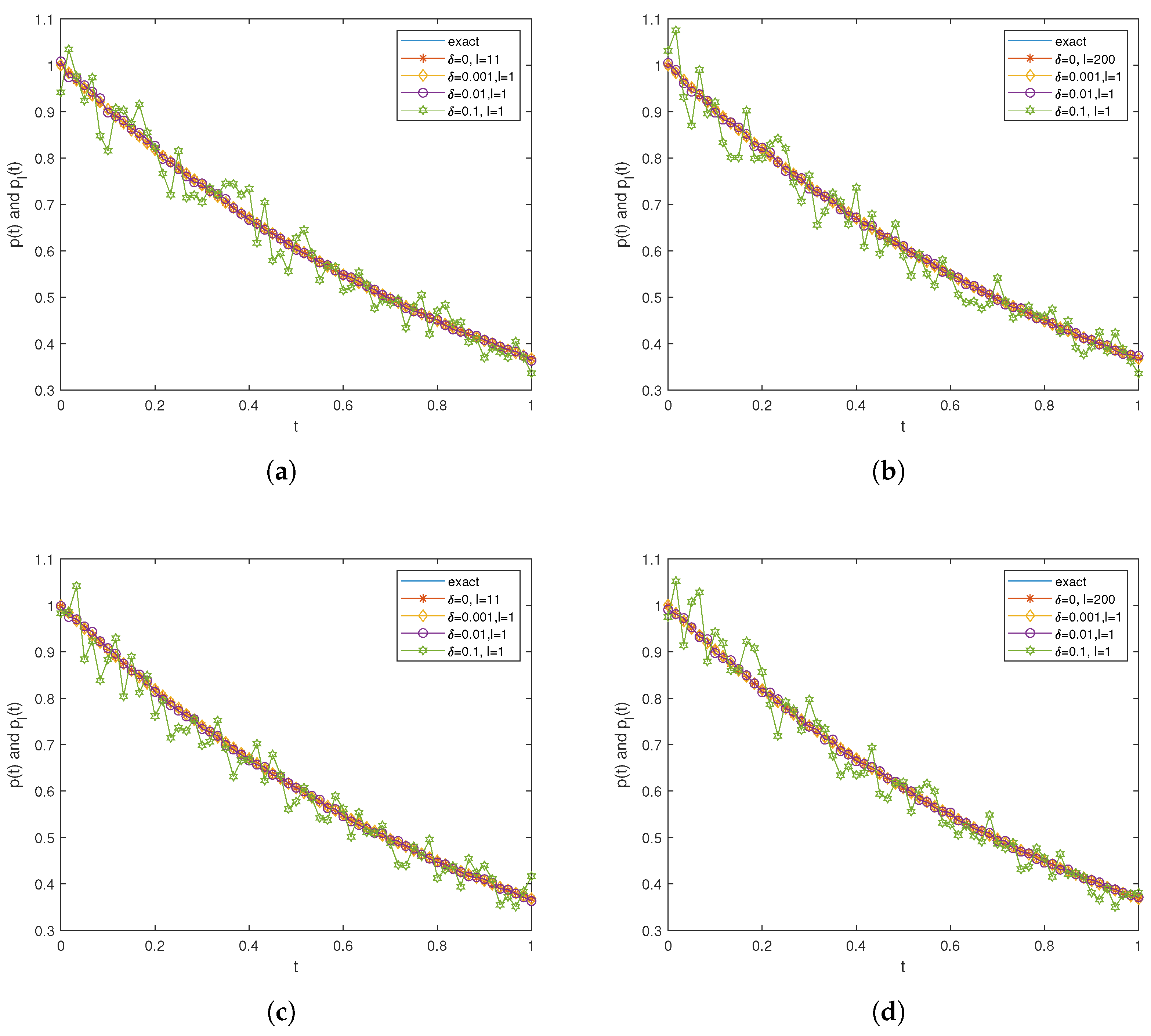
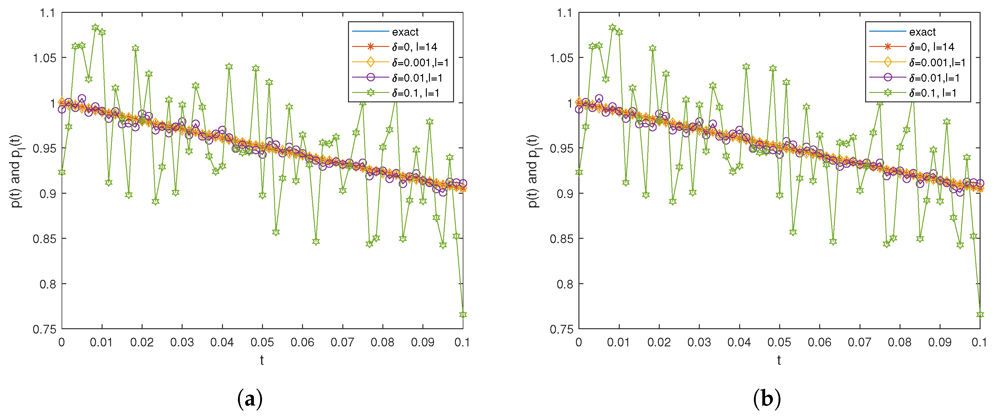
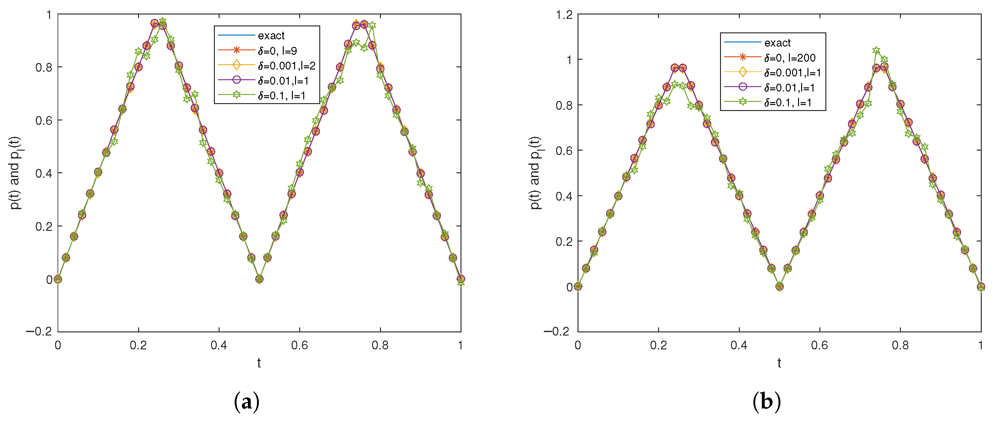
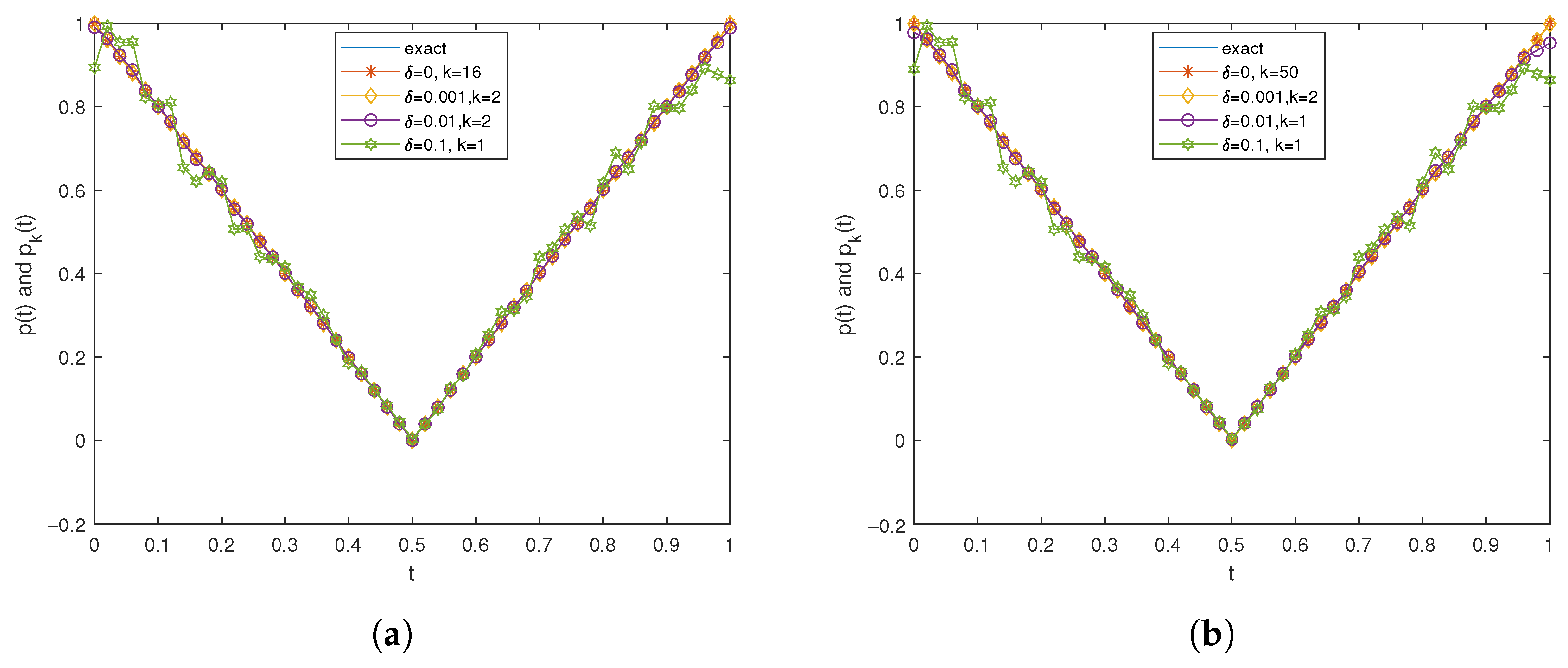
• One-dimensional case We consider three types of examples: continuous smooth monotonic decreasing functions, functions with sharp points, and discontinuous step functions. We compare the images corresponding to two values of $\beta$, namely, $\beta =1.2$ and $\beta =1.8$. Additionally, the root mean square error (RMSE) is defined as follows:

  $$R(p)={\left({\displaystyle \frac{{\displaystyle \sum _{i=1}^M}{\left(p^{(l)}(t_i)-p(t_i)\right)}^2}{{\displaystyle \sum _{i=1}^M}p{(t_i)}^2}}\right)}^{{\displaystyle \frac{1}{2}}}.$$

Example 1. 

Let $a(x)=0$, $\mu (\alpha )=\Gamma (5-\alpha )$ and the space source function $f(x)=x^2$ and the time source function $p(t)=e^{-t}$.

Figure 1 presents the inversion results of a rapidly decreasing function for $\beta =1.2$ and $\beta =1.8$. The numerical solutions exhibit excellent agreement with the exact solutions for both $\beta$ values. However, when the noise level increases to $\delta =0.1$, the fitting accuracy between the numerical and exact solutions decreases. This discrepancy arises primarily due to the ill-posed nature of the inverse problem, where only single-point data are utilized to reconstruct the temporal source term, combined with the accelerated decay characteristics of the function. Despite these challenges, the observed errors are deemed acceptable, demonstrating the stability and effectiveness of the proposed algorithm.

Figure 1. Results of Example 1 corresponding to different noise levels: (a) $\theta =0$, $\beta =1.2.$ (b) $\theta =0$, $\beta =1.8.$ (c) $\theta =0.001{\epsilon }^2$, $\beta =1.2$. (d) $\theta =0.001{\epsilon }^2$, $\beta =1.8$.

Additionally, under strong noise conditions ($\delta =0.1$), the number of iterations required to meet the stopping criterion is only one, which further highlights the algorithm’s rapid convergence and robust inversion performance. These experimental results indicate that the proposed algorithm achieves computational efficiency and numerical stability across varying noise levels, ensuring high-precision numerical solutions for spatial source term inversion. Based on the above analysis, we adopt $\theta =0$ in subsequent numerical experiments. For Figure 1, we compared the inversion images under two distinct noise-contaminated datasets. First, for the case of $\theta =0$, Figure 1a,b display the results corresponding to $\beta =1.2$ and $\beta =1.8$, respectively. From these figures, we observe that when the noise level $\delta =0$, the iteration count for $\beta =1.2$ was $l=11$, whereas for $\beta =1.8$, it required $l=200$ iterations. This demonstrates that the iteration speed for $\beta =1.8$ is faster compared to $\beta =1.2$. When the noise data were set to $\delta =0.001$, $0.01$, or $0.1$, the iteration count reached the stopping criterion of the discrepancy principle after only one iteration. Similarly, with $\theta =0.001$ fixed, the iteration speed of $\beta =1.2$ remained faster than that of $\beta =1.8$, while other scenarios aligned with the $\theta =0$ case.

Table 1 presents the RMSE for different regularization parameters and $\beta$ values, which are used to assess the quality of the results. We fixed $\theta =0$ and calculated the RMSE for $\beta =1.1,1.3,1.5,1.7,1.9$ and calculated the RMSE for $\beta =1.3$, with a value of 0.0602. while the minimum RMSE of 0.0548 was achieved at $\beta =1.7$. The difference between these two values was only 0.0054. This indicates that the choice of $\beta$ is not sensitive in the problem of identifying the time-dependent source term, and our data remain stable under variations in $\beta$. Similarly, when we fixed $\theta =0.001{\epsilon }^2$, we observed that the maximum RMSE was 0.0573 at $\beta =1.3$, while the minimum RMSE of 0.0517 was obtained at $\beta =1.9$, with a difference of only 0.0056. The same conclusion can be drawn in this scenario as well.

Table 1. RMSE table for the case of $\delta =0.1$.

$\mathit{\beta }$	1.1	1.3	1.5	1.7	1.9
$R(p)$$,\theta =0$	0.0548	0.0602	0.0560	0.0579	0.0593
$R(p)$$,\theta =0.001{\epsilon }^2$	0.0536	0.0558	0.0573	0.0565	0.0517

According to Figure 1, there is no significant difference between the computational results for $\theta =0$ and $\theta =0.001{\epsilon }^2$. Specifically, regardless of which value of $\theta$ is chosen, the obtained numerical solutions show very similar performance in terms of both accuracy and convergence. This indicates that, in the context of this problem, the choice of the parameter $\theta$ has little impact on the final results. Therefore, in the subsequent examples and numerical experiments, we will focus on analyzing the case of $\theta =0$ in order to simplify the analysis and reduce the computational effort. This approach not only helps to highlight the main features of the method but also makes the results more representative and comparable.

Figure 2 presents the numerical results for $\beta =1.2$ and $\beta =1.8$ at $T=0.1$. As can be seen from the figure, due to the extremely slow dynamics exhibited by the distributed-order time-space diffusion equation over a relatively short time interval, the numerical results deteriorate more noticeably at $T=0.1$ compared to $T=1$ when the noise level is high. This phenomenon is also consistent with the characteristics of superslow diffusion—this is also an important direction to consider in the future.

Figure 2. Results of Example 1 corresponding to different noise levels: (a) $T=0.1$, $\beta =1.2.$ (b) $T=0.1$, $\beta =1.8.$

Example 2. 

Testing a source term functions with sharp points. Let $f(x)=cos(\pi x)$, $\mu (\alpha )=\Gamma (4-\alpha )$, and $a(x)=x^{2+\beta }{(1-x)}^{2+\beta }$. Choose $p(t)$ as follows:

$$p(t)=\left\{\begin{array}{cc}4t,& t\in [0,{\displaystyle \frac{1}{4}}),\hfill \\ 2-4t,& t\in [{\displaystyle \frac{1}{4}},{\displaystyle \frac{1}{2}}),\hfill \\ -2+4t,& t\in [{\displaystyle \frac{1}{2}},{\displaystyle \frac{3}{4}}),\hfill \\ 4-4t,& t\in [{\displaystyle \frac{3}{4}},1).\hfill \end{array}\right.$$

(49)

Analysis of Figure 3 reveals that the numerical solutions exhibit excellent agreement with the exact solutions when $\delta \le 0.01$. However, at $\delta =0.1$, slight deviations emerge in the fitting accuracy between the two curves. These deviations originate from the non-differentiability of the function at singular points, which induces instability in the numerical solutions. Despite these localized discrepancies, the overall results remain largely unaffected. Such minor differences are deemed acceptable and fully demonstrate the robustness and efficacy of the proposed algorithm.

Figure 3. Results of Example 2 corresponding to different noise levels: (a) $\theta =0$, $\beta =1.2.$ (b) $\theta =0$, $\beta =1.8.$

Example 3. 

Let us consider a piecewise function as an example, where the source term is

$$p(t)=\left\{\begin{array}{cc}7,& t\in [0,{\displaystyle \frac{1}{4}}),\hfill \\ 5,& t\in [{\displaystyle \frac{1}{4}},{\displaystyle \frac{1}{2}}),\hfill \\ 3,& t\in [{\displaystyle \frac{1}{2}},{\displaystyle \frac{3}{4}}),\hfill \\ 1,& t\in [{\displaystyle \frac{3}{4}},1).\hfill \end{array}\right.$$

(50)

Let $f(x)=cos(\pi x)$ and $a(x)=x^2{(1-x)}^2$, $\mu (\alpha )=\Gamma (5-\alpha )$.

Figure 4 presents the inversion results of a piecewise function. Analysis reveals that the numerical solutions exhibit good agreement with the exact solutions when $\delta \le 0.01$. However, under a higher noise level ($\delta =0.1$), a clear instability in the numerical solutions becomes evident. This instability is primarily attributed to the discontinuities inherent in the piecewise function, which propagate uncertainties in the numerical computations. These observations underscore the challenges in maintaining numerical stability for functions with discontinuities during the inversion process.

Figure 4. Results of Example 3 corresponding to different noise levels: (a) $\theta =0$, $\beta =1.2.$ (b) $\theta =0$, $\beta =1.8.$

• Two-dimensional case To demonstrate the effectiveness of the proposed method, two illustrative examples have been selected for validation in this paper. In these examples, we fix the $\mu =\Gamma (2-\alpha )$, rather than blindly analyzing numerical examples.

Example 4. 

Let the source function $p(t)=2sin(4\pi t)+exp(-t)+t$, $f(x,y)=cos(2\pi x)$$cos(2\pi y)+{\displaystyle \frac{1}{10}}$ and $a(x,y)=x(1-x)+y(1-y)$. The specific results are shown in Figure 5.

Figure 5. Results of Example 4 corresponding to different noise levels: (a) $\theta =0$, $\beta =1.2.$ (b) $\theta =0$, $\beta =1.8.$

Figure 5 illustrates the numerical inversion results for a two-dimensional smooth function. The results demonstrate that significant numerical instabilities are observed in regions with high curvature when $\delta =0.1$, indicating heightened sensitivity of these areas to noise perturbations. In contrast, the numerical solutions exhibit excellent agreement with the exact solutions in regions of low curvature, highlighting the algorithm’s robust stability in smoother domains. This phenomenon not only validates the effectiveness of the proposed method but also identifies critical challenges for further algorithmic refinement.

Example 5. 

We consider a function with a sharp point, $p(t)=|2t-1|$, where the source function $f(x,y)=cos(2\pi x)cos(2\pi y)+{\displaystyle \frac{1}{10}}{e}^{-{\displaystyle \frac{1}{3}}(x^3-3x^2)(2y^3-3y^2)}$ and the initial data are $a(x,y)=x^{2+{\displaystyle \frac{\beta }{2}}}{(1-x)}^{2+{\displaystyle \frac{\beta }{2}}}+y^{2+{\displaystyle \frac{\beta }{2}}}{(1-y)}^{2+{\displaystyle \frac{\beta }{2}}}$. The specific results are shown in Figure 6.

Figure 6. Results of Example 5 corresponding to different noise levels: (a) $\theta =0$, $\beta =1.2.$ (b) $\theta =0$, $\beta =1.8.$

Figure 6 demonstrates the inversion of a piecewise function with discontinuous features. The results show that, despite pronounced jump discontinuities in the target function at interface points, the proposed algorithm effectively reconstructs its fundamental structure. Notably, the numerical solutions exhibit satisfactory agreement with the exact solutions for noise levels $\delta \le 0.01$. While instability arises in the numerical results at $\delta =0.1$, the deviations remain confined within acceptable bounds and display a distinct convergence trend as iterations proceed. These findings conclusively validate that our method is not only applicable to smooth functions but also demonstrates robust adaptability and numerical stability for discontinuous piecewise function reconstructions.

In conclusion, based on the numerical examples presented, it can be observed that both the one-dimensional and two-dimensional algorithms are applicable to functions of any type. This observation serves as evidence that our algorithm, along with the theoretical support provided in this paper, is accurate and reliable.

8. Discussion

This paper investigates the inverse problem of determining a time-dependent source term in distributed-order time-space fractional differential equations. The existence and uniqueness of the solution to the direct problem, as well as the uniqueness of the inverse problem, are rigorously established. By employing the conjugate gradient method in conjunction with Tikhonov regularization, we efficiently solve the inverse problem. Five numerical examples, including both one- and two-dimensional cases, demonstrate that the proposed method achieves high accuracy, robustness, and stability, even with noisy data.

A notable advantage of our approach lies in the combination of rigorous theoretical analysis and effective numerical implementation, which ensures both reliability and practical applicability. Moreover, the algorithm maintains good computational efficiency for moderate problem sizes. Nevertheless, one current limitation is that, as the noise level in the additional data increases, relatively large errors may appear at the endpoints, possibly due to accumulated errors in solving the direct, sensitivity, and adjoint problems.

To further improve the computational efficiency and scalability of our method, especially for large-scale or high-dimensional problems, we plan to incorporate advanced techniques such as hierarchical matrices and adaptive cross approximation, which can significantly reduce both memory requirements and computational cost. Additionally, studying the inverse problem with the time-fractional derivative order $\alpha \in (1,2)$ is also of great importance and will be an important direction in our future research.

References

- Caputo, M. Mean fractional-order-derivatives differential equations and filters. Annali dell’Universita di Ferrara 1995, 41, 73–84. [Google Scholar] [CrossRef]
- Mainardi, F.; Mura, A.; Pagnini, G.; Gorenflo, R. Time-fractional diffusion of distributed order. J. Vib. Control 2008, 14, 1267–1290. [Google Scholar] [CrossRef]
- Sokolov, I.M.; Chechkin, A.V.; Klafter, J. Natural and Modified Forms of Distributed-Order Fractional Diffusion Equations; Fractional Dynamics: Recent Advances; World Scientific Publishing: Hackensack, NJ, USA, 2012; pp. 107–127. [Google Scholar]
- Bu, W.P.; Ji, L.; Tang, Y.F.; Zhou, J. Space-time finite element method for the distributed-order time fractional reaction diffusion equations. Appl. Numer. Math. 2020, 152, 446–465. [Google Scholar] [CrossRef]
- Habibirad, A.; Azin, H.; Hesameddini, E. A capable numerical meshless scheme for solving distributed order time-fractional reaction-diffusion equation. Chaos Soliton Fract. 2023, 166, 112931. [Google Scholar] [CrossRef]
- Mohammadi-Firouzjaeiand, H.; Adibi, H.; Dehghan, M. Local discontinuous Galerkin method for distributed-order time-fractional diffusion-wave equation: Application of laplace transform. Math. Methods Appl. Sci. 2021, 44, 4923–4937. [Google Scholar] [CrossRef]
- Jia, J.H. Analysis of a hidden-memory variably distributed-order time-fractional diffusion equation. Fractal Fract. 2022, 6, 627. [Google Scholar] [CrossRef]
- Sandev, T.; Tomovski, Z.; Crnkovic, B. Generalized distributed order diffusion equations with composite time fractional derivative. Comput. Math. Appl. 2017, 73, 1028–1040. [Google Scholar] [CrossRef]
- Jiang, D.J.; Li, Z.Y.; Liu, Y.; Yamamoto, M. Weak unique continuation property and a related inverse source problem for time-fractional diffusion-advection equations. Inverse Probl. 2017, 33, 055013. [Google Scholar] [CrossRef]
- Jin, B.T.; Rundell, W. A tutorial on inverse problems for anomalous diffusion processes. Inverse Probl. 2015, 31, 035003. [Google Scholar] [CrossRef]
- Sakamoto, K.; Yamamoto, M. Initial value/boundary value problems for fractional diffusion-wave equations and applications to some inverse problems. J. Math. Anal. Appl. 2011, 382, 426–447. [Google Scholar] [CrossRef]
- Yan, X.B.; Wei, T. Inverse space-dependent source problem for a time-fractional diffusion equation by an adjoint problem approach. J. Inverse Ill-Posed Probl. 2019, 27, 1–16. [Google Scholar] [CrossRef]
- Jin, B.T.; Kian, Y. Recovery of a distributed order fractional derivative in an unknown medium. Commun. Math. Sci. 2023, 21, 1791–1813. [Google Scholar] [CrossRef]
- Liu, J.J.; Sun, C.L.; Yamamoto, M. Recovering the weight function in distributed order fractional equation from interior measurement. Appl. Numer. Math. 2021, 168, 84–103. [Google Scholar] [CrossRef]
- Rundell, W.; Zhang, Z.D. Fractional diffusion: Recovering the distributed fractional derivative from overposed data. Inverse Probl. 2017, 33, 035008. [Google Scholar] [CrossRef]
- Li, Z.Y.; Fujishiro, K.; Li, G.S. Uniqueness in the inversion of distributed orders in ultraslow diffusion equations. J. Comput. Appl. Math. 2020, 369, 112564. [Google Scholar] [CrossRef]
- Ruan, Z.S.; Wang, Z.W. A backward problem for distributed order diffusion equation: Uniqueness and numerical solution. Inverse Probl. Sci. Eng. 2021, 29, 418–439. [Google Scholar] [CrossRef]
- Yuan, L.L.; Cheng, X.L.; Liang, K.W. Solving a backward problem for a distributed-order time fractional diffusion equation by a new adjoint technique. J. Inverse Ill-Posed Probl. 2020, 28, 471–488. [Google Scholar] [CrossRef]
- Jiang, D.J.; Li, Z.Y. Coefficient inverse problem for variable order time-fractional diffusion equations from distributed data. Calcolo 2022, 59, 34. [Google Scholar] [CrossRef]
- Ma, W.J.; Sun, L.L. Inverse potential problem for a semilinear generalized fractional diffusion equation with spatio-temporal dependent coefficients. Inverse Probl. 2023, 39, 015005. [Google Scholar] [CrossRef]
- Zhang, M.M.; Liu, J.J. Identification of a time-dependent source term in a distributed-order time-fractional equation from a nonlocal integral observation. Comput. Math. Appl. 2019, 78, 3375–3389. [Google Scholar] [CrossRef]
- Sun, C.L.; Liu, J.J. An inverse source problem for distributed order time-fractional diffusion equation. Inverse Probl. 2020, 36, 055008. [Google Scholar] [CrossRef]
- Hai, D.N.D. Identifying a space-dependent source term in distributed order time-fractional diffusion equations. Math. Control Relat. Fields 2023, 13, 1008–1022. [Google Scholar] [CrossRef]
- Kubica, A.; Ryszewska, K. Decay of solutions to parabolic-type problem with distributed order Caputo derivative. J. Math. Anal. Appl. 2018, 465, 79–99. [Google Scholar] [CrossRef]
- Lischke, A.; Pang, G.; Gulian, M.; Song, F.; Glusa, C.; Zheng, X.; Mao, Z.; Cai, W.; Meerschaert, M.M.; Ainsworth, M.; et al. What is the fractional Laplacian? A comparative review with new results. J. Comput. Phys. 2020, 404, 109009. [Google Scholar] [CrossRef]
- Tatar, S.; Tnaztepe, R.; Ulusoy, S. Simultaneous inversion for the exponents of the fractional time and space derivatives in the space-time fractional diffusion equation. Appl. Anal. 2016, 95, 1–23. [Google Scholar] [CrossRef]
- Tatar, S.; Tnaztepe, R.; Ulusoy, S. Determination of an unknown source term in a space-time fractional diffusion equation. J. Fract. Calc. Appl. 2015, 6, 83–90. [Google Scholar]
- Tatar, S.; Ulusoy, S. An inverse source problem for a one-dimensional space-time fractional diffusion equation. Appl. Anal. 2015, 94, 2233–2244. [Google Scholar] [CrossRef]
- Ilic, M.; Liu, F.; Turner, I.; Anh, V. Numerical approximation of a fractional-in-space diffusion equation. II-with nonhomogeneous boundary conditions. Fract. Calc. Appl. Anal. 2006, 9, 333–349. [Google Scholar]
- Cheng, X.L.; Yuan, L.L.; Liang, K.W. Inverse source problem for a distributed-order time fractional diffusion equation. J. Inverse Ill-Posed Probl. 2020, 28, 17–32. [Google Scholar] [CrossRef]
- Kilbas, A.A.A.; Srivastava, H.M.; Trujillo, J.J. Theory and Applications of Fractional Differential Equations; Elsevier Science Limited: Amsterdam, The Netherlands, 2006; Volume 204. [Google Scholar]
- Brezis, H. Functional Analysis, Sobolev Spaces and Partial Differential Equations; Springer: Berlin/Heidelberg, Germany, 2011; Volume 2. [Google Scholar]
- Kirsch, A. An Introduction to the Mathematical Theory of Inverse Problems, 2nd ed.; Springer: New York, NY, USA, 2011. [Google Scholar]
- Wang, H.M.; Li, Y.S. Numerical solution of backward problem of distributed order time-space fractional diffusion equation. Phys. Scr. 2025, 100, 025252. [Google Scholar] [CrossRef]
- Aimi, A.; Desiderio, L.; Credico, G.D. Partially pivoted ACA based acceleration of the energetic BEM for time-domain acoustic and elastic waves exterior problems. Comput. Math. Appl. 2022, 119, 351–370. [Google Scholar] [CrossRef]
- Morozov, V.A. Methods for Solving Incorrectly Posed Problems; Springer: New York, NY, USA, 1984. [Google Scholar]
Disclaimer/Publisher’s Note: The statements, opinions and data contained in all publications are solely those of the individual author(s) and contributor(s) and not of MDPI and/or the editor(s). MDPI and/or the editor(s) disclaim responsibility for any injury to people or property resulting from any ideas, methods, instructions or products referred to in the content. |
© 2025 by the authors. Licensee MDPI, Basel, Switzerland. This article is an open access article distributed under the terms and conditions of the Creative Commons Attribution (CC BY) license (https://creativecommons.org/licenses/by/4.0/).