Formation Control of Underactuated AUVs Using a Fractional-Order Sliding Mode Observer

Abstract

This paper proposes a control method that combines a fractional-order sliding mode observer and a cooperative control strategy to address the problem of path-following for underactuated autonomous underwater vehicles (AUVs) in complex marine environments. First, a fractional-order sliding mode observer is designed, combining fractional calculus and double-power convergence laws to enhance the estimation accuracy of high-frequency disturbances. An adaptive gain mechanism is introduced to avoid dependence on the upper bound of disturbances. Second, a formation cooperative control strategy based on path parameter coordination is proposed. By setting independent reference points for each AUV and exchanging path parameters, formation consistency is achieved with low communication overhead. For the followers’ speed control problem, an error-based expected speed adjustment mechanism is introduced, and a hyperbolic tangent function is used to replace the traditional arctangent function to improve the response speed of the system. Numerical simulation results show that this control method performs well in terms of path-following accuracy, formation maintenance capability, and disturbance suppression, verifying its effectiveness and robustness in complex marine environments.

1. Introduction

As the development of marine resources continues to advance, unmanned underwater vehicles (UUVs) are playing an increasingly critical role in deep-sea exploration, marine rescue, and resource exploration missions [1,2,3]. Compared with single autonomous underwater vehicles (AUVs), multi-AUV cooperative operations can not only complete complex tasks that are difficult for a single AUV to accomplish independently but also improve the overall efficiency and reliability of the mission. However, due to the complexity of the underwater environment, the underactuated characteristics of AUVs, and the limitations of underwater acoustic communication, multi-AUV formation control faces many challenges [4,5,6]. To address these issues, the academic community has conducted extensive research and proposed various formation control strategies, primarily including leader–follower methods [7,8,9,10,11,12,13], consensus control methods [14,15,16,17], virtual structure methods [18,19], and behavior-based methods [20,21,22].

In the leader–follower strategy, the leader AUV guides the formation movement, while the remaining AUVs act as followers, adjusting their own states based on the leader’s position and speed to maintain the formation structure [7,8]. However, in practical applications, due to noise interference and communication delays, it is difficult to accurately obtain the leader’s speed information. To reduce reliance on velocity information, references [9,10,13] introduced virtual inputs, enabling formation control based solely on the leader’s position information, thereby reducing the amount of information exchange between AUVs. Additionally, references [11,12] further introduced the concept of “virtual vehicles”, using virtual targets to assist in designing the follower controller, thereby enhancing the system’s robustness and feasibility. Yu et al. proposed an event-triggered consistency control protocol combining the artificial potential field method [14], effectively reducing communication frequency, but the design of the event-triggered mechanism is relatively complex. Tao et al. utilized graph theory models combined with adaptive backstepping sliding mode control strategies to achieve system consistency [15]. Reference [16] applied graph theory to multi-AUV formations, achieving individual state synchronization through local neighbor information. Reference [17] addresses communication delays by proposing a consensus control algorithm that simultaneously utilizes relative position and velocity information; however, control performance still needs improvement under conditions of severe delay fluctuations. The virtual structure method treats the entire AUV formation as a rigid whole rather than a collection of independent entities. This approach does not require the designation of a specific leader, thereby avoiding formation disintegration caused by single-point failures [18]. However, this method typically relies on globally accurate information and may be constrained by actual communication conditions in long-range communication or complex environments. Reference [19] proposes a composite control strategy that integrates virtual structure and artificial potential field technologies, further enhancing the system’s environmental adaptability and obstacle avoidance capabilities. Behavior-driven methods achieve collaborative control of the overall system by combining the basic behaviors of individual AUVs. Reference [20] optimizes the system’s navigation performance and dynamic response capabilities through behavior strategies. References [21,22] utilized this method to achieve formation control and target detection tasks for multiple AUVs, demonstrating the autonomy and coordination of multi-AUV systems when executing complex tasks.

In practical applications, AUVs often face complex and unpredictable external disturbances, which place higher demands on the robustness and stability of control systems. To address external disturbances, uncertainties, and noise, researchers have developed various control strategies, including common methods such as adaptive control, sliding mode control, and neural network control, aimed at enhancing the system’s tracking and formation-maintaining performance under disturbance conditions. For example, references [23,24] propose a sliding mode control strategy based on a nonlinear disturbance observer, utilizing dynamic compensation methods for the online estimation of lumped disturbances, thereby enhancing the system’s robustness. References [25,26] address dynamic uncertainty by designing an extended state observer for observation and compensation, proposing an adaptive terminal sliding mode control scheme. References [27,28] utilize adaptive radial basis function neural networks to achieve online learning and estimation of system disturbances, improving the system’s interference resistance. Fractional calculus has garnered significant attention in the control field due to its ability to characterize dynamic features with memory and hereditary properties. Compared to traditional integer-order models, fractional-order systems are more accurate in characterizing the complex dynamic behavior of physical systems, and fractional-order controllers offer greater flexibility in parameter tuning, thereby demonstrating significant advantages in high-precision control tasks [29,30,31]. Specifically, references [30,31] propose a sliding mode control method based on a fractional-order disturbance observer, which not only improves disturbance estimation accuracy but also effectively reduces the common chattering issues in sliding mode control. Reference [32] extends fractional-order sliding mode control to discrete-time systems and utilizes the memory characteristics of fractional-order differences to enhance the disturbance resistance of motor systems. References [33,34], respectively, improved the dynamic response performance of motor systems and spatial robotic arms by designing fractional-order integral sliding mode surfaces and non-singular terminal sliding mode control laws. Additionally, references [35,36] combined high-gain observers with neural network methods to achieve efficient disturbance estimation and event-triggered control in multi-agent systems. Reference [37] proposes an adaptive sliding mode disturbance observer based on the Caputo derivative to enhance the system’s adaptability to disturbances. In terms of composite control strategies, reference [38] integrates fuzzy neural networks with fractional-order sliding mode observers to improve harmonic suppression capabilities, while reference [39] utilizes the Nussbaum gain function to address the issue of unknown control directions in fractional-order interconnected systems.

In summary, although previous studies have achieved certain results in multi-AUV formation control and interference suppression, there are still shortcomings in terms of high-frequency disturbance estimation accuracy and underwater communication efficiency. In response to these issues, this paper focuses on the formation tracking control of underactuated AUVs in complex marine environments, with an emphasis on improvements in disturbance observer design and cooperative control strategies with low communication traffic to enhance the system’s adaptability to complex disturbances and strengthen the practical feasibility of multi-AUV collaboration. The main work is as follows:

(1)

Fractional-order sliding mode observer design: A fractional-order sliding mode observer (FOSMO) is proposed, combining fractional calculus with a double-power approximation law. The fractional-order operator enhances the system’s response capability to high-frequency disturbances, while the double-power approximation law effectively suppresses sliding mode chattering. Additionally, an adaptive gain regulation mechanism is introduced to ensure the system maintains good estimation accuracy and robustness even under unknown disturbance upper-bound conditions.

(2)

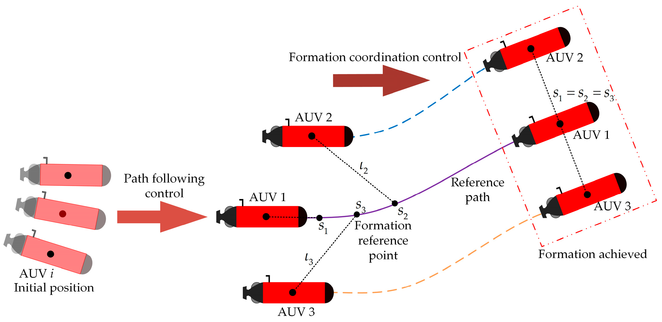
Formation cooperative control strategy: For multi-AUV formation tasks, a cooperative control strategy based on path parameter negotiation is designed. This method assigns each AUV an independent formation reference point and achieves cooperative consistency through the exchange of path parameters rather than state information, reducing communication requirements and improving the strategy’s adaptability in bandwidth-constrained underwater environments.

(3)

Speed adjustment mechanism optimization: For the speed control of follower AUVs, an expected speed adjustment method based on error feedback is proposed. This method uses a hyperbolic tangent function to replace the arctangent function, providing smoother adjustment responses in small error intervals and accelerating system convergence under large error conditions, thereby improving overall control performance and response efficiency.

The structure of the paper is as follows: Section 2 models and describes the problem, including the kinematic and dynamic modeling of underactuated AUVs and the mathematical formalization of formation control tasks. Section 3 details the design process of the controller and observer and performs a system stability analysis. Section 4 validates the effectiveness and robustness of the proposed control strategy through numerical simulation experiments and includes an analysis of the results and a comparative discussion. Finally, Section 5 provides a summary of the entire paper and an outlook for future work.

2. Problem Description

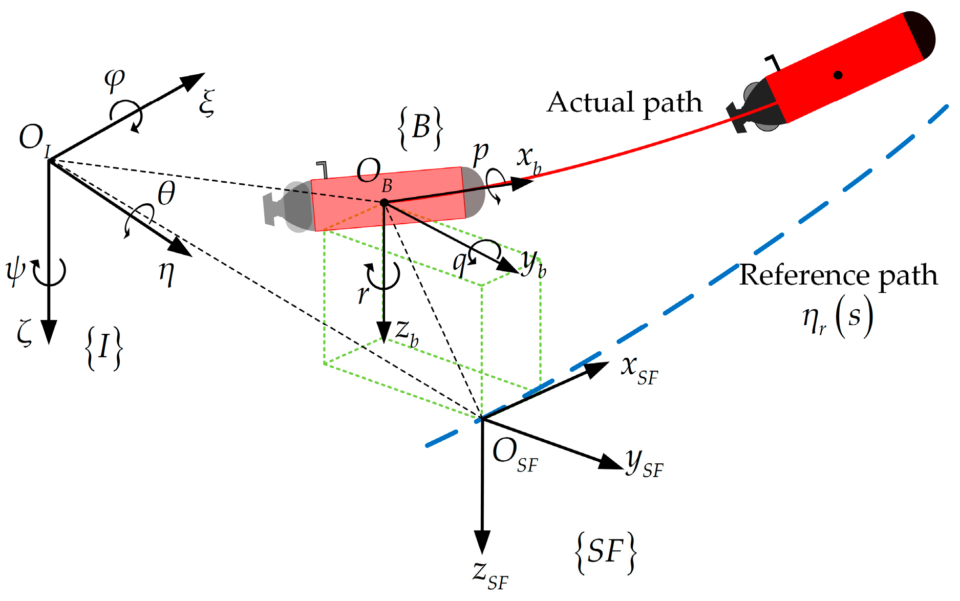
2.1. AUV Model

This section derives the path-following error model of an underactuated AUV in three-dimensional space. First, the coordinate system and related symbols used are defined, followed by the kinematic and dynamic models of the AUV. Based on this, the mathematical expression of the three-dimensional path-following error is given.

As shown in Figure 1, the body coordinate system $\left\{B\right\}:O_B-x_b{y}_b{z}_b$, the Earth coordinate system $\left\{I\right\}:O_I-\xi \eta \zeta$, and the path coordinate system $\left\{SF\right\}:O_{SF}-x_{SF}{y}_{SF}{z}_{SF}$ are defined. The kinematic and dynamic models of the AUV are given as follows [40]:

$$\left\{\begin{array}{l}\dot{\eta }=J\left(\eta \right)v_r+v_c\\ M{\dot{v}}_r+C\left(v_r\right)v_r+D\left(v_r\right)v_r+g\left(\eta \right)=\tau +{\tau }_d\end{array}\right.$$

(1)

Assumption 1.

The AUV prototype under study has a uniformly distributed body mass, with gravity and buoyancy forces in equilibrium. Nonlinear hydrodynamic damping terms and the effects of roll motion are neglected in the model.

Assumption 2.

The origin of the body coordinate system coincides with the center of gravity.

Assumption 3.

The disturbance vector ${\tau }_d$ is unknown but bounded, and its rate of change is also unknown but bounded.

Assumption 4.

Roll motion and higher-order hydrodynamic damping terms of the AUV are neglected.

Based on these assumptions, the three-dimensional motion equations of the AUV can be described as follows:

$$\left\{\begin{array}{l}\dot{x}=u_r\cos \psi \cos \theta -v_r\sin \psi +w_r\cos \psi \sin \theta +u_{c\xi }\\ \dot{y}=u_r\sin \psi \cos \theta +v_r\cos \psi +w_r\sin \psi \sin \theta +v_{c\eta }\\ \dot{z}=-u_r\sin \theta +w_r\cos \theta +w_{c\zeta }\\ \dot{\theta }=q\\ \dot{\psi }=r/\cos \theta \end{array}\right.$$

(2)

$$\left\{\begin{array}{l}{\dot{u}}_r={\displaystyle \frac{m_2}{m_1}}{v}_{r}r-{\displaystyle \frac{m_3}{m_1}}{w}_{r}q-{\displaystyle \frac{d_1}{m_1}}{u}_r+{\displaystyle \frac{{\tau }_X+{\tau }_{du}}{m_1}}\hfill \\ {\dot{v}}_r=-{\displaystyle \frac{m_1}{m_2}}{u}_{r}r-{\displaystyle \frac{d_2}{m_2}}{v}_r+{\displaystyle \frac{{\tau }_{dv}}{m_2}}\hfill \\ {\dot{w}}_r={\displaystyle \frac{m_1}{m_3}}{u}_{r}q-{\displaystyle \frac{d_3}{m_3}}{w}_r+{\displaystyle \frac{{\tau }_{dw}}{m_3}}\hfill \\ \dot{q}=-{\displaystyle \frac{m_1-m_3}{m_4}}{u}_r{w}_r-{\displaystyle \frac{d_4}{m_4}}q-{\displaystyle \frac{M_g}{m_4}}+{\displaystyle \frac{{\tau }_M+{\tau }_{dq}}{m_4}}\hfill \\ \dot{r}={\displaystyle \frac{m_1-m_2}{m_5}}{u}_r{v}_r-{\displaystyle \frac{d_5}{m_5}}r+{\displaystyle \frac{{\tau }_N+{\tau }_{dr}}{m_5}}\hfill \end{array}\right.$$

(3)

where $x$, $y$, and $z$ represent the position of the AUV in the Earth coordinate system, and $\theta$ and $\psi$ denote the attitude of the AUV. $v_r={\left[u_r v_r w_r q r\right]}^{\mathrm{T}}$ is the velocity vector of the AUV relative to the water flow, and $v_c={\left[u_{cx}{v}_{ch}{w}_{cz}0 0 0\right]}^{\mathrm{T}}$ represents the velocity vector of the water flow in the Earth coordinate system. $J\left(\eta \right)$ is the transformation matrix from $\left\{B\right\}$ to $\left\{I\right\}$. $M={\left[m_1{m}_2{m}_3{m}_4{m}_5\right]}^{\mathrm{T}}$ is the inertia matrix. $C\left(v_r\right)$ is the Coriolis and centrifugal force matrix. $D\left(v_r\right)={\left[d_1 d_2 d_3 d_4 d_5\right]}^{\mathrm{T}}$ is the damping matrix, and $g\left(\eta \right)={\left[0 0 0 M_g 0\right]}^{\mathrm{T}}$ is the restoring torque matrix. $\tau ={\left[{\tau }_X 0 0 {\tau }_M {\tau }_N\right]}^{\mathrm{T}}$ is the control input vector of the AUV. ${\tau }_d={\left[{\tau }_{du} {\tau }_{dv} {\tau }_{dw} {\tau }_{dq} {\tau }_{dr}\right]}^{\mathrm{T}}$ represents the disturbance vector composed of unknown environmental disturbances and unmodeled parts of the AUV.

Define the reference path as ${\eta }_r\left(s\right)={\left[x_f{y}_f{z}_f {\theta }_f {\psi }_f\right]}^{\mathrm{T}}$, the position and attitude of the AUV in the $\left\{I\right\}$ coordinate system as $P={\left[xyz \theta \psi \right]}^{\mathrm{T}}$, the position following error in the $\left\{SF\right\}$ coordinate system as ${\left[x_e y_e z_e\right]}^{\mathrm{T}}=R_1\left[\eta -{\eta }_r\left(s\right)\right]$, and the attitude error as ${\left[{\theta }_e {\psi }_e\right]}^{\mathrm{T}}={\left[\theta +\alpha -{\theta }_f \cos {\theta }_f\left(\psi +\beta -{\psi }_f\right)\right]}^{\mathrm{T}}$. The derivative of the position error can be derived as follows:

$$\left\{\begin{array}{l}{\dot{x}}_e={\dot{\psi }}_f{y}_e-{\dot{\theta }}_f{z}_e+U\cos {\psi }_e\cos {\theta }_e-u_f\\ {\dot{y}}_e=-{\dot{\psi }}_f{x}_e-{\dot{\psi }}_f\tan {\theta }_f{z}_e+U\sin {\psi }_e\cos {\theta }_e\\ {\dot{z}}_e={\dot{\theta }}_f{x}_e+{\dot{\psi }}_f\tan {\theta }_f{y}_e-U\sin {\theta }_e\end{array}\right.$$

(4)

where $\alpha =-\arctan \left({\displaystyle \frac{w}{u}}\right)$, $\beta =\arctan \left({\displaystyle \frac{v}{u}}\right)$, and $U=\sqrt{u^2+v^2+w^2}$. $R_1$ is the transformation matrix from $\left\{I\right\}$ to $\left\{SF\right\}$, $R_1=\left[\begin{array}{ccc}\cos {\psi }_f\cos {\theta }_f& \sin {\psi }_f& -\cos {\psi }_f\sin {\theta }_f\\ -\sin {\psi }_f\cos {\theta }_f& \cos {\psi }_f& \sin {\psi }_f\sin {\theta }_f\\ \sin {\theta }_f& 0& \cos {\theta }_f\end{array}\right]$. $u_f$ is the velocity of the reference point on the reference path.

Assumption 5.

The reference path is known and is twice continuously differentiable. The path is parameterized by the arc length parameter s.

2.2. Control Objective

In order to achieve the cooperative formation control of multiple AUV systems, it is first necessary to ensure that each AUV can accurately follow its respective reference path and then achieve overall formation coordination through a cooperative mechanism. This paper assigns an independent formation reference point to each AUV and uses a negotiation mechanism to gradually align their respective reference points, thereby achieving the desired formation. Let the formation vector of the i-th AUV relative to the reference point be ${\iota }_i={\left[{\iota }_{xi}{\iota }_{yi} {\iota }_{zi}\right]}^{\mathrm{T}}$; then, their reference paths are expressed as

$${\eta }_{r,i}\left(s_i\right)={\eta }_r\left(s_i\right)+R_2{\iota }_i$$

(5)

where $R_2$ is the transformation matrix from $\left\{B\right\}$ to $\left\{I\right\}$.

When all reference points are in agreement, each AUV will maintain stable navigation in the desired formation [7,16]. The control strategy adjusts the speed of each AUV so that its actual speed gradually approaches the desired speed, thereby promoting the convergence of each reference point and ultimately achieving a stable formation structure. The control objective can be expressed based on the convergence of path-following errors, achieving reference point consistency between each AUV to maintain formation. The mathematical description is as follows:

$$\underset{t\to \infty }{\lim }\left|{\eta }_i-{\eta }_{r,i}\left(s_i\right)\right|=0,\forall i\in \left\{1,2,\dots n\right\}$$

(6)

$$\underset{t\to \infty }{\lim }\left|U_{ri}-U_d\right|=0,\forall i\in \left\{1,2,\dots n\right\}$$

(7)

Equation (6) represents the path-following target of a single AUV, ensuring convergence to the reference path and formation position. Equation (7) represents the synchronization target, enabling follower AUVs to catch up with the leader.

3. Following Controller Design

The design principle of the path-following controller is shown in Figure 2. The design of the controller is divided into two key steps:

• Kinematic Controller Design: The integral line-of-sight (ILOS) method is used to compensate for path deviations caused by ocean currents. Based on this, a kinematic controller is constructed using the backstepping method. By adjusting the navigation heading angle to stabilize the position error, the desired velocity control law and angular velocity control law for the path reference point are derived. These laws provide reference signals for subsequent dynamic control.
• Dynamic Controller Design: To enhance system robustness, a fractional-order sliding mode observer is designed to estimate disturbances, modeling errors, and other lumped uncertainties. The desired velocity output from the kinematic controller serves as a reference signal. Combined with the introduced desired forward velocity, an integral sliding mode control method is employed to design the control law, thereby achieving precise control of the AUV.

3.1. Kinematic Controller Design

For underactuated vehicles, due to the lack of lateral and vertical thrusters, it is impossible to provide direct lateral or vertical thrust. Therefore, this paper uses the ILOS method [23,41,42] to introduce a navigation angle to stabilize the position error. The navigation angle is given as follows:

$$\left\{\begin{array}{l}{\theta }_{\mathrm{nav}}=\arctan \left({\displaystyle \frac{z_e}{{\Delta }_{\theta }}}-\widehat{\alpha }\right)+{\theta }_f\\ {\psi }_{\mathrm{nav}}=-\arctan \left({\displaystyle \frac{y_e}{{\Delta }_{\psi }}}+\widehat{\beta }\right)+{\psi }_f\end{array}\right.$$

(8)

where ${\Delta }_{\theta }$ and ${\Delta }_{\psi }$ are the forward-looking distances and are considered constants in the ILOS method.

Let $\theta ={\theta }_{\mathrm{nav}}$, $\psi ={\psi }_{\mathrm{nav}}$. Substituting Equation (8) into Equation (4) yields

$$\left\{\begin{array}{l}{\dot{x}}_e={\dot{\psi }}_f{y}_e-{\dot{\theta }}_f{z}_e+U\cos {\psi }_e\cos {\theta }_e-u_f\\ {\dot{y}}_e=-{\dot{\psi }}_f{x}_e-{\dot{\psi }}_f\tan {\theta }_f{z}_e+U\sin \left(\cos {\theta }_f\left({\psi }_{\mathrm{nav}}+\beta -{\psi }_f\right)\right)\cos {\theta }_e\\ {\dot{z}}_e={\dot{\theta }}_f{x}_e+{\dot{\psi }}_f\tan {\theta }_f{y}_e-U\sin \left({\theta }_{\mathrm{nav}}+\alpha -{\theta }_f\right)\end{array}\right.$$

(9)

The speed control law of the design reference point and the expected angular velocity control law of the AUV are as follows:

$$u_f=U\cos {\psi }_e\cos {\theta }_e+k_1{x}_e$$

(10)

$$\left\{\begin{array}{l}{q}_d=-k_{\theta }\tilde{\theta }+{\dot{\theta }}_{\mathrm{nav}}\\ r_d=\cos \theta (-k_{\psi }\tilde{\psi }+{\dot{\psi }}_{\mathrm{nav}})\end{array}\right.$$

(11)

where $\tilde{\theta }=\theta -{\theta }_{\mathrm{nav}}$, $\tilde{\psi }=\psi -{\psi }_{\mathrm{nav}}$.

The adaptive law for design parameters is

$$\left\{\begin{array}{l}\dot{\widehat{\alpha }}=-{\displaystyle \frac{k_{\alpha }{z}_e{\Delta }_{\theta }}{\sqrt{{\Delta }_{\theta }^2+{\left(z_e-{\Delta }_{\theta }\widehat{\alpha }\right)}^2}}}\\ \dot{\widehat{\beta }}={\displaystyle \frac{k_{\beta }{y}_e{\Delta }_{\psi }\cos {\theta }_e}{\sqrt{{\Delta }_{\psi }^2+{\left(y_e+{\Delta }_{\psi }\widehat{\beta }\right)}^2}}}\end{array}\right.$$

(12)

where $k_1$, $k_{\theta }$, $k_{\psi }$, $k_{\alpha }$, and $k_{\beta }$ are proportional coefficients, all of which are greater than zero.

Note 1.

$\alpha$, $\beta$, and ${\theta }_f$ are relatively small; therefore, $\cos \alpha \approx 1$, $\sin \alpha \approx \alpha$, $\sin \beta \approx \beta$, and $\cos {\theta }_f\approx 1$.

Theorem 1.

For the error model described by Equation (4), we first introduce the navigation angle defined in Equation (8), transforming the lateral and vertical position errors into an attitude error stabilization problem. Based on this transformation, we design a reference point velocity control law, with its explicit form given in Equation (10). The AUV kinematic control law is then specified in Equation (11), and the parameter adaptation law is presented in Equation (12). Together, these ensure that the system error converges to the equilibrium point, provided the reference point velocity control law and the AUV kinematic control law satisfy the conditions of Barbalat’s lemma.

Proof of Theorem 1.

A Lyapunov function is designed as follows:

$$V_1={\displaystyle \frac{1}{2}}{x_e}^2+{\displaystyle \frac{1}{2}}{y_e}^2+{\displaystyle \frac{1}{2}}{z_e}^2+{\displaystyle \frac{1}{2}}{\tilde{\theta }}^2+{\displaystyle \frac{1}{2}}{\tilde{\psi }}^2+{\displaystyle \frac{U}{2k_{\alpha }}}{\tilde{\alpha }}^2+{\displaystyle \frac{U}{2k_{\beta }}}{\tilde{\beta }}^2$$

(13)

We then take the derivative of Equation (13), which yields

$$\begin{array}{l}{\dot{V}}_1=x_e{\dot{x}}_e+y_e{\dot{y}}_e+z_e{\dot{z}}_e+\tilde{\theta }\dot{\tilde{\theta }}+\tilde{\psi }\dot{\tilde{\psi }}-{\displaystyle \frac{U\tilde{\alpha }\dot{\widehat{\alpha }}}{k_{\alpha }}}-{\displaystyle \frac{U\tilde{\beta }\dot{\widehat{\beta }}}{k_{\beta }}}\\ =x_e\left(U\cos {\psi }_e\cos {\theta }_e-u_f\right)+y_{e}U\sin \left(-\arctan \left({\displaystyle \frac{y_e}{{\Delta }_{\psi }}}+\widehat{\beta }\right)+\beta \right)\cos {\theta }_e\\ -z_{e}U\sin \left(\arctan \left({\displaystyle \frac{z_e}{{\Delta }_{\theta }}}-\widehat{\alpha }\right)+\alpha \right)+\tilde{\theta }\dot{\tilde{\theta }}+\tilde{\psi }\dot{\tilde{\psi }}-{\displaystyle \frac{U\tilde{\alpha }\dot{\widehat{\alpha }}}{k_{\alpha }}}-{\displaystyle \frac{U\tilde{\beta }\dot{\widehat{\beta }}}{k_{\beta }}}\\ =x_e\left(U\cos {\psi }_e\cos {\theta }_e-u_f\right)-{\displaystyle \frac{U{z}_e\left(z_e-{\Delta }_{\theta }\widehat{\alpha }\right)}{\sqrt{{\Delta }_{\theta }^2+{\left(z_e-{\Delta }_{\theta }\widehat{\alpha }\right)}^2}}}-{\displaystyle \frac{U{z}_e{\Delta }_{\theta }\alpha }{\sqrt{{\Delta }_{\theta }^2+{\left(z_e-{\Delta }_{\theta }\widehat{\alpha }\right)}^2}}}\\ -{\displaystyle \frac{U{y}_e\left(y_e+{\Delta }_{\psi }\widehat{\beta }\right)\cos {\theta }_e}{\sqrt{{\Delta }_{\psi }^2+{\left(y_e+{\Delta }_{\psi }\widehat{\beta }\right)}^2}}}+{\displaystyle \frac{U{y}_e{\Delta }_{\psi }\beta \cos {\theta }_e}{\sqrt{{\Delta }_{\psi }^2+{\left(y_e+{\Delta }_{\psi }\widehat{\beta }\right)}^2}}}+\tilde{\theta }\left(q-{\dot{\theta }}_{nav}\right)+\tilde{\psi }\left({\displaystyle \frac{r}{\cos \theta }}-{\dot{\psi }}_{nav}\right)-{\displaystyle \frac{U\tilde{\alpha }\dot{\widehat{\alpha }}}{k_{\alpha }}}-{\displaystyle \frac{U\tilde{\beta }\dot{\widehat{\beta }}}{k_{\beta }}}\end{array}$$

(14)

Bringing Equations (10)–(12) into Equation (14) yields

$${\dot{V}}_1=-k_1{x}_e^2-{\displaystyle \frac{U{z}_e^2}{\sqrt{{\Delta }_{\theta }^2+{\left(z_e-{\Delta }_{\theta }\widehat{\alpha }\right)}^2}}}-{\displaystyle \frac{U{y}_e^2\cos {\theta }_e}{\sqrt{{\Delta }_{\psi }^2+{\left(y_e+{\Delta }_{\psi }\widehat{\beta }\right)}^2}}}-k_{\theta }{\tilde{\theta }}^2-k_{\psi }{\tilde{\psi }}^2$$

(15)

The constructed energy function $V_1$ is a positive definite function, and its derivative ${\dot{V}}_1$ is negative semi-definite. According to Barbalat’s lemma, it can be inferred that the system error will gradually converge to zero over time, thereby ensuring the asymptotic stability of the system. □

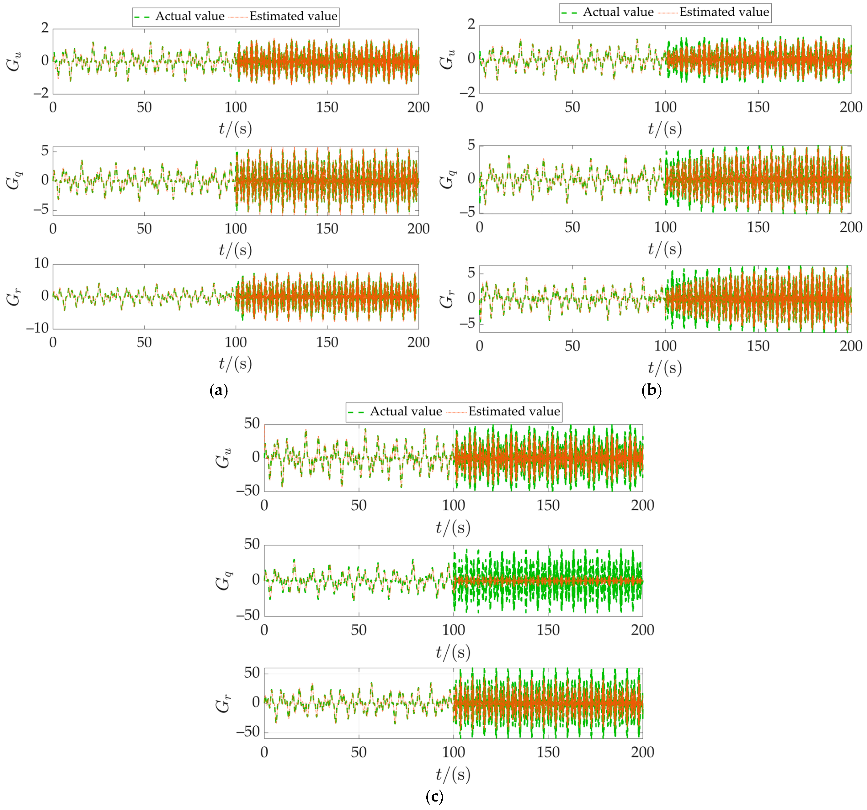
3.2. Fractional-Order Sliding Mode Disturbance Observer Design

By integrating the fractional calculus theory and double-power approximation law, this study proposes a new type of sliding mode disturbance observer. This observer utilizes the non-local memory characteristics of fractional calculus to enhance the ability to capture high-frequency disturbances and time-varying characteristics of unmodeled dynamics in underactuated AUV systems. It is particularly suitable for accurately estimating random disturbances in underwater environments and improving the system’s robustness to high-frequency disturbances. Additionally, by incorporating the double-power convergence law, the observer can dynamically adjust the convergence speed near the sliding surface, thereby optimizing convergence performance. Furthermore, the introduction of an adaptive gain regulation mechanism eliminates reliance on prior knowledge of disturbance upper bounds, enabling real-time compensation for system dynamic changes through online updates of gain parameters.

Define system uncertainty and unknown time-varying disturbances as $G\left(v_r\right)=-M^{-1}\left(C\left(v_r\right)v_r+D\left(v_r\right)v_r+g\left(\eta \right)-{\tau }_d\right)$, thereby rewriting Equation (1) as

$${\dot{v}}_r=G\left(v_r\right)+M^{-1}\tau$$

(16)

The observed value is expressed as ${\dot{\widehat{v}}}_r=\widehat{G}\left(v_r\right)+M^{-1}\tau$, the observation error is ${\tilde{v}}_r=v_r-{\widehat{v}}_r$, and the sliding mode surface is designed as

$$\Omega =k_s{\tilde{v}}_r+{\mathrm{D}}^m\left({\tilde{v}}_r\right)+{\dot{\tilde{v}}}_r$$

(17)

where $k_s>0$, $-1<m<0$.

Note 2.

The fractional order is defined using the Riemann–Liouville definition, which takes the form

$${\mathrm{D}}^m\left(f\left(t\right)\right)={\displaystyle \frac{1}{\mathrm{G}\left(n-m\right)}}{\displaystyle \frac{d^n}{d{t}^n}}{\displaystyle {\int }_0^t\frac{f\left(\tau \right)}{{\left(t-\tau \right)}^{1+m-n}}}\mathrm{d}\tau$$

(18)

where  $\mathrm{G}\left(m\right)={\displaystyle {\int }_0^{\infty }{\exp }^{-t}{t}^{m-1}}\mathrm{d}t$ is the gamma function [31,43].

Assumption 6.

Disturbances and the vehicle’s velocity are both bounded. As a result, an unknown upper bound exists for the compound disturbances.

The sliding mode reaching law is designed as follows:

$$\dot{\Omega }=-{\mu }_1{\left|\Omega \right|}^p\mathrm{sgn}\left(\Omega \right)-{\mu }_2{\left|\Omega \right|}^q\mathrm{sgn}\left(\Omega \right)-{\mu }_3\Omega$$

(19)

where ${\mu }_1>0$, ${\mu }_2>0$, and ${\mu }_3>0$ are gain parameters. $0<p<1$, $1<q$.

A fractional-order sliding mode observer and parameter adaptive law are designed as follows:

$$\dot{\widehat{G}}\left(v\right)={\mathrm{D}}^{m+1}\left({\tilde{v}}_r\right)+k_s{\dot{\tilde{v}}}_r+\widehat{\omega }\mathrm{sgn}\left(\Omega \right)+{\mu }_1{\left|\Omega \right|}^p\mathrm{sgn}\left(\Omega \right)+{\mu }_2{\left|\Omega \right|}^q\mathrm{sgn}\left(\Omega \right)+{\mu }_3\Omega$$

(20)

$$\dot{\widehat{\omega }}=\lambda \left|\Omega \right|$$

(21)

where $\lambda >0$ and $\omega$ is the unknown upper bound of the disturbance.

Theorem 2.

For the AUV system in Equation (16), the sliding mode observer is designed as in Equation (20). The disturbance estimation error of the proposed FOSMO is guaranteed to be stable if the adaptive law for the disturbance upper bound follows the form given in Equation (21).

Proof of Theorem 2.

A Lyapunov function is designed as follows:

$$V_2={\displaystyle \frac{1}{2}}{\Omega }^2+{\displaystyle \frac{1}{2\lambda }}{\tilde{\omega }}^2$$

(22)

We then take the derivative of Equation (22), bringing Equations (20) and (21) into it, yielding

$$\begin{array}{l}{\dot{V}}_2=\Omega \dot{\Omega }-{\displaystyle \frac{\tilde{\omega }\dot{\widehat{\omega }}}{\lambda }}\\ =\Omega \left(k_s{\dot{\tilde{v}}}_r+{\mathrm{D}}^{m+1}\left({\tilde{v}}_r\right)+\dot{G}\left(v_r\right)-\dot{\widehat{G}}\left(v_r\right)\right)-\tilde{\omega }\left|\Omega \right|\\ =\Omega \left(\dot{G}\left(v_r\right)-\widehat{\omega }\mathrm{sgn}\left(\Omega \right)\right)-{\mu }_1{\left|\Omega \right|}^{p+1}-{\mu }_2{\left|\Omega \right|}^{q+1}-{\mu }_3{\Omega }^2-\tilde{\omega }\left|\Omega \right|\\ \le \tilde{\omega }\left|\Omega \right|-{\mu }_1{\left|\Omega \right|}^{p+1}-{\mu }_2{\left|\Omega \right|}^{q+1}-{\mu }_3{\Omega }^2--\tilde{\omega }\left|\Omega \right|=-{\mu }_1{\left|\Omega \right|}^{p+1}-{\mu }_2{\left|\Omega \right|}^{q+1}-{\mu }_3{\Omega }^2\end{array}$$

(23)

Since ${\dot{V}}_2<0$, the observer is stable, and the system state converges to the sliding mode surface in finite time. Thus, the system can estimate the disturbance value in finite time. □

3.3. Dynamic Controller Design

Define the desired speed variable as $V_d={\left[u_d q_d r_d\right]}^{\mathrm{T}}$ and the speed error variable as

$$E_i=\left\{\begin{array}{l}{u}_e=u_r-u_d\\ q_e=q-q_d\\ r_e=r-r_d\end{array}\right.$$

(24)

The sliding mode surface is designed as

$$S_i=h_{1i}{E}_i+h_{2i}{\displaystyle {\int }_0^t{E}_i\mathrm{d}t}$$

(25)

where $h_{1i}>0$, $h_{2i}>0$. The sliding mode reaching law is designed as follows:

$${\dot{S}}_i=-b_{1i}{\left|S_i\right|}^{{\gamma }_i}\mathrm{sgn}\left(S_i\right)-b_{2i}{S}_i$$

(26)

where $b_{1i}>0$, $b_{2i}>0$, $0<{\gamma }_i<1$.

The control law is designed as follows:

$$\left\{\begin{array}{l}\tau =M\left(-\widehat{G}\left(v_r\right)+{\dot{V}}_d-{\widehat{\Phi }}_i\mathrm{sgn}\left(S_i\right)+\left(-h_{2i}{E}_i-b_{1i}{\left|S_i\right|}^{{\gamma }_i}\mathrm{sgn}\left(S_i\right)-b_{2i}{S}_i\right)/h_{1i}\right)\\ {\dot{\widehat{\Phi }}}_i=h_{1i}{k}_{\Phi i}\left|S_i\right|\end{array}\right.$$

(27)

where $k_{\Phi i}>0$ and ${\Phi }_i$ is the upper bound of the observer’s observation error.

Theorem 3.

For the underactuated AUV model described by Equation (1), the path-following problem is transformed into an error stabilization problem. To cope with external disturbances and unknown system dynamics in the model, a fractional-order sliding mode observer as shown in Equation (20) is designed to achieve accurate observation and compensation of the system state. The kinematic control law is determined by Equation (11). On this basis, a sliding mode control method is used to design the dynamic control law as shown in Equation (27). The error will asymptotically converge to the equilibrium point if the control law (27) satisfies the condition of Barbalat’s lemma. Thus, under these conditions, the AUV achieves asymptotic path-following, validating the control design.

Proof of Theorem 3.

A Lyapunov function is designed as follows:

$$V_3={\displaystyle \frac{1}{2}}{S_i}^2+{\displaystyle \frac{1}{2k_{\Phi i}}}{{\tilde{\Phi }}_i}^2$$

(28)

We then take the derivative of Equation (28), bringing Equation (27) into it, yielding

$$\begin{array}{l}{\dot{V}}_3=S_i\left(h_{1i}\left(G\left(v_r\right)+M^{-1}\tau -{\dot{V}}_d\right)+h_{2i}{E}_i\right)-{\tilde{\Phi }}_i{\dot{\widehat{\Phi }}}_i/k_{\Phi i}\\ =S_i\left(h_{1i}\left(\tilde{G}\left(v_r\right)-{\widehat{\Phi }}_i\mathrm{sgn}\left(S_i\right)\right)-b_{1i}{\left|S_i\right|}^{{\gamma }_i}\mathrm{sgn}\left(S_i\right)-b_{2i}{S}_i\right)-h_{1i}\left|S_i\right|{\tilde{\Phi }}_i\\ \le h_{1i}\left|S_i\right|{\Phi }_i-h_{1i}\left|S_i\right|{\widehat{\Phi }}_i-b_{1i}{\left|S_i\right|}^{{\gamma }_i+1}-b_{2i}{S_i}^2-h_{1i}\left|S_i\right|{\tilde{\Phi }}_i=-b_{1i}{\left|S_i\right|}^{{\gamma }_i+1}-b_{2i}{S_i}^2\end{array}$$

(29)

The constructed energy function $V_3$ is a positive definite function, and its derivative ${\dot{V}}_3$ is negative semi-definite. According to Barbalat’s lemma, it can be inferred that the system error will gradually converge to zero over time, thereby ensuring the asymptotic stability of the system. □

4. Formation Coordination Controller Design

4.1. Principles of Controller Design

This study uses the leader–follower method for multi-AUV coordination, designating one AUV as the leader and the rest as followers. The leader’s path is preset, while followers’ paths are generated by translating and compressing the leader’s path to meet formation requirements. Building on the controller from Section 3, which converts single AUV path-following into a position and velocity stabilization problem, this chapter’s formation coordination controller further transforms formation maintenance into a velocity control problem. The leader specifies the desired velocity and employs a control law to drive the pose error vector to zero, ensuring convergence to the set path. For followers, the generalized distance to the leader is calculated, and their velocity is dynamically adjusted via velocity control to form and maintain the desired geometric formation.

In traditional formation control, followers adjust their velocities based on the position and velocity information transmitted from the lead AUV, which demands substantial communication bandwidth and is impractical for underwater scenarios with limited communication capacity [16]. To tackle this, this paper presents a formation control strategy that only requires exchanging path parameters, effectively reducing communication needs. As illustrated in Figure 3, the formation control process involves the two following steps:

• Each AUV executes its path-following control law to ensure its trajectory stably converges to the assigned path. This precise spatial control forms the foundation of formation coordination.
• Based on information exchange between robots, a coordination control law is designed to dynamically adjust followers’ expected speed values. This enables temporal coordination within the formation, achieving a stable and orderly formation configuration.

For clarity, the leader and followers are denoted as l and f, respectively, in the subsequent text. Parameters with l or f subscripts correspond to those related to the leader or followers, respectively.

4.2. Coordination Controller Design

The leader AUV only requires path-following control, and the desired speed $U_{l,d}$ is directly given. The speed control law of the leader reference point and the desired angular velocity control law of the leader AUV are designed as follows:

$$u_{l,f}=U_l\cos {\psi }_{l,e}\cos {\theta }_{l,e}+k_{l,1}{x}_{l,e}$$

(30)

$$\left\{\begin{array}{l}{q}_{l,d}=-k_{l,\theta }{\tilde{\theta }}_l+{\dot{\theta }}_{l,nav}-{\dot{\alpha }}_l+{\dot{\theta }}_{l,f}\\ r_{l,d}=\cos {\theta }_l(-k_{l,\psi }{\tilde{\psi }}_l+{\dot{\psi }}_{l,nav}-{\dot{\beta }}_l+{\dot{\psi }}_{l,f})\end{array}\right.$$

(31)

The controller and adaptive law are designed as follows:

$$\left\{\begin{array}{l}{\tau }_l=M\left({\dot{U}}_{l,d}-{\widehat{G}}_l\left(v_r\right)-{\widehat{\Phi }}_{l,i}\mathrm{sgn}\left(S_{l,i}\right)-\left(h_{l,2i}{E}_{l,i}+b_{l,1i}{\left|S_{l,i}\right|}^{{\gamma }_{l,i}}\mathrm{sgn}\left(S_{l,i}\right)+b_{l,2i}{S}_{l,i}\right)/h_{l,1i}\right)\\ {\dot{\widehat{\Phi }}}_{l,i}=h_{l,1i}{k}_{l,\Phi i}\left|S_{l,i}\right|\end{array}\right.$$

(32)

The controller design for the follower is similar to that of the leader, but there is a key difference: the expected speed of the leader is directly specified, while the expected speed of the follower is designed based on the generalized distance between the leader and the follower’s reference point in order for the follower to catch up with the leader. Specifically, the generalized distance can be expressed by the arc length parameter as

$$\tilde{s}=s_l-s_f$$

(33)

The expected speed of followers can be designed as follows:

$$U_{f,d}=U_{l,d}+k_{\Delta }\tanh \left(\tilde{s}\right)-\iota$$

(34)

Note 3.

The inverse tangent function is commonly used for speed adjustment in references [7,16,44]. However, its smoother and slower growth in response to large errors can limit the correction amplitude, especially in the initial formation stage, potentially slowing convergence. Therefore, this paper introduces the hyperbolic tangent function for speed adjustment. Comparison with $\arctan \left(b\right)$: when $b\to 0$, the first-order derivative of $\tanh \left(b\right)$ is 1, whereas the derivative of $\arctan \left(b\right)$ is ${\displaystyle \frac{1}{1+b^2}}\le 1$. This means that for small tracking errors, the hyperbolic tangent function provides a steeper gradient for adjustment compared to the inverse tangent function, which leads to faster convergence in formation control. The $\tanh \left(b\right)$ rapidly saturates to ±1 when $\left|b\right|>2$, while $\arctan \left(b\right)$ approaches ±π/2 more slowly. This property ensures that the hyperbolic tangent function constrains the control action within [−1,1], preventing excessively aggressive corrections for large errors. Therefore, this paper adopts the hyperbolic tangent function for speed regulation. Compared to arctan, tanh achieves a balanced response: it avoids over-adjustment in small error regions while ensuring sufficiently strong corrective action in the presence of large errors, which effectively accelerates system convergence and enhances overall control performance and responsiveness.

In the same way, the speed control law of the follower reference point and the expected angular velocity control law of the follower AUV are as follows:

$$u_{f,f}=U_f\cos {\psi }_{f,e}\cos {\theta }_{f,e}+k_{f,1}{x}_{f,e}$$

(35)

$$\left\{\begin{array}{l}{q}_{f,d}=-k_{f,\theta }{\tilde{\theta }}_f+{\dot{\theta }}_{f,nav}-{\dot{\alpha }}_f+{\dot{\theta }}_{f,f}\\ r_{f,d}=\cos {\theta }_f(-k_{f,\psi }{\tilde{\psi }}_f+{\dot{\psi }}_{f,nav}-{\dot{\beta }}_f+{\dot{\psi }}_{f,f})\end{array}\right.$$

(36)

The controller and adaptive law are designed as follows:

$$\left\{\begin{array}{l}{\tau }_f=M\left({\dot{U}}_{f,d}-{\widehat{G}}_f\left(v_r\right)-{\widehat{\Phi }}_{f,i}\mathrm{sgn}\left(S_{f,i}\right)-\left(h_{f,2i}{E}_{f,i}+b_{f,1i}{\left|S_{f,i}\right|}^{{\gamma }_{f,i}}\mathrm{sgn}\left(S_{f,i}\right)+b_{f,2i}{S}_{f,i}\right)/h_{f,1i}\right)\\ {\dot{\widehat{\Phi }}}_{f,i}=h_{f,1i}{k}_{f,\Phi i}\left|S_{f,i}\right|\end{array}\right.$$

(37)

Theorem 4.

For the underactuated AUV model described in Equation (1), the formation reference path is given by Equation (5). For the leader, the control law shown in Equation (32) is designed; for the follower, the control law shown in Equation (37) is used. Given the desired speed of the leader, the desired speed control law of the follower shown in Equation (34) is further designed. If the designed control laws ensure that the system satisfies the conditions required by Barbalat’s lemma, it follows that the formation tracking errors will asymptotically converge to zero. This guarantees that the multi-AUV system not only follows the desired path but also maintains a stable formation configuration.

Proof of Theorem 4.

A Lyapunov function is designed as follows:

$$V_{l,f}={\displaystyle \frac{1}{2}}{\tilde{s}}^2+{\displaystyle \frac{1}{2}}{\left(U_{l,d}-U_{f,d}\right)}^2$$

(38)

as pointed out in reference [16], the instantaneous velocity of s is the desired velocity of the AUV. Therefore, we take the derivative of Equation (38), which yields

$${\dot{V}}_{l,f}=\tilde{s}\left(U_{l,d}-U_{f,d}\right)+\left(U_{l,d}-U_{f,d}\right)\left({\dot{U}}_{l,d}-{\dot{U}}_{f,d}\right)=-k_{\Delta }\tilde{s}\tanh \left(\tilde{s}\right)-k_{\Delta }\left(1-{\tanh }^2\left(\tilde{s}\right)\right){\left(U_{l,d}-U_{f,d}\right)}^2\le 0$$

(39)

where $k_{\Delta }>0$. For all matrices $\tilde{s}\ne 0$ and $\left(U_{l,d}-U_{f,d}\right)\ne 0$, there exists ${\dot{V}}_{l,f}<0$; this ensures that the system is asymptotically stable. □

5. Numerical Simulation and Result Analysis

To comprehensively verify the proposed control scheme, simulation experiments were conducted for two case studies. The simulation parameters were based on the AUV prototype model constructed by the team. For specific parameters, please refer to [23,24,45]. Case 1 verified the path-following capability of a single AUV, and Case 2 verified the formation transformation and maintenance capability of multiple AUVs.

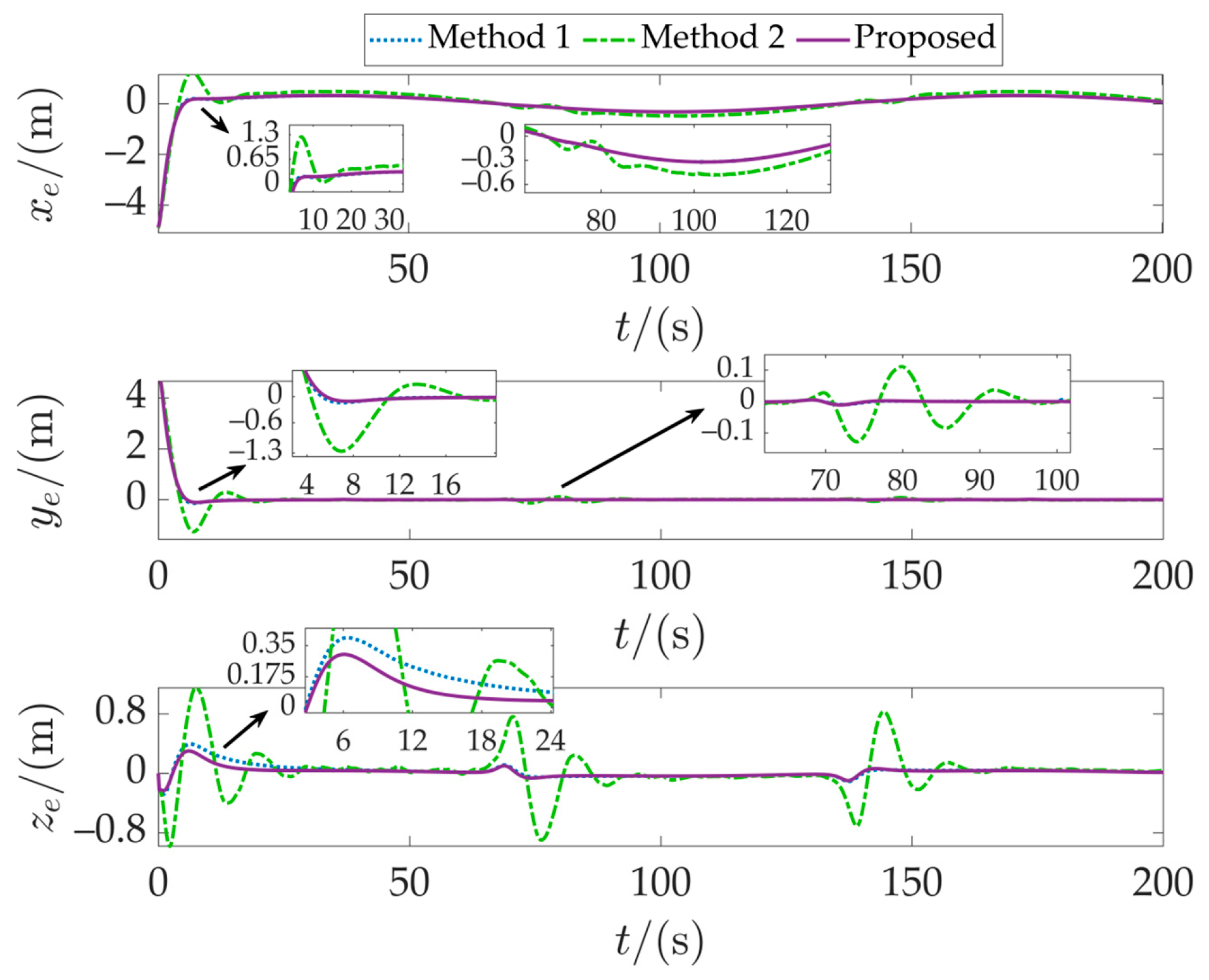
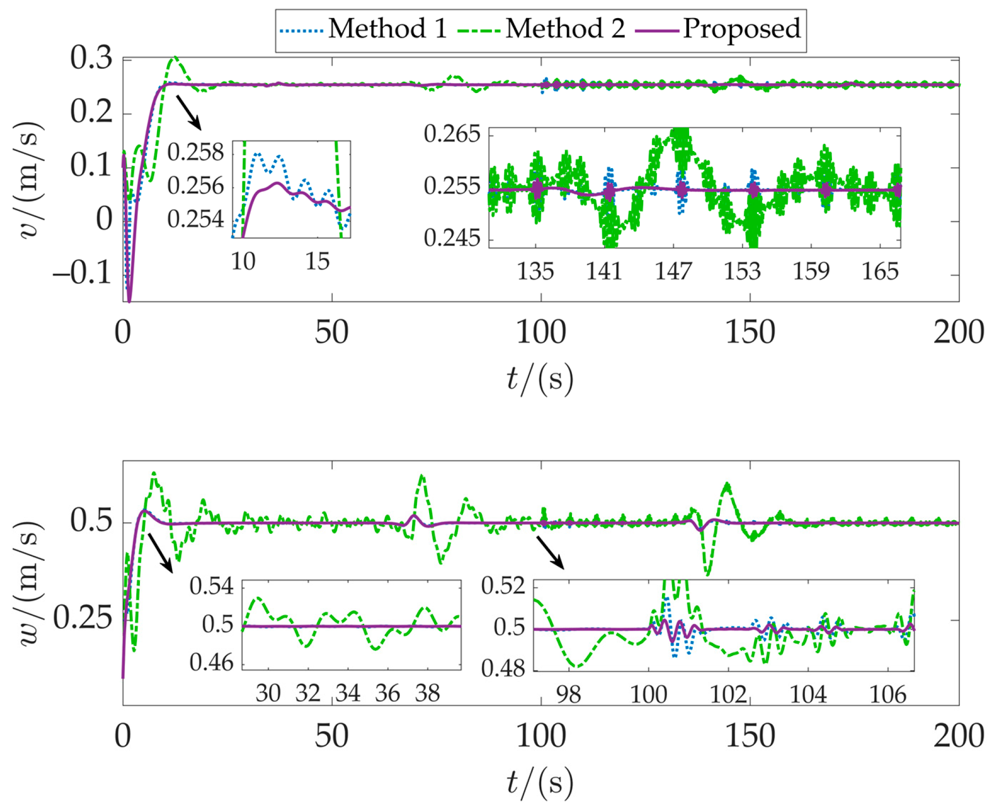
5.1. Case 1: Single AUV Path-Following

This case simulates the path-following performance of a single AUV in a constant ocean current environment. The performance of three control methods in terms of tracking performance, disturbance estimation capability, and robustness is compared and analyzed. The comparison methods are as follows:

Method 1: Disturbance estimation based on a linear approach law sliding mode observer, combined with the ILOS guidance law and integral sliding mode control.

Method 2: Perturbation estimation based on a nonlinear disturbance observer, combined with the ILOS guidance law and integral sliding mode control.

Method 3 (the method used in this paper): Perturbation estimation based on a fractional-order sliding mode observer, combined with the ILOS guidance law and integral sliding mode control.

The reference path is a spatial spiral curve, whose parametric equation is as follows:

$$\left\{\begin{array}{l}{x}_f\left(s\right)=45\cos \left(0.1 s\right)\\ y_f\left(s\right)=45\sin \left(0.1s\right)\\ z_f\left(s\right)=0.5 s\end{array}\right.$$

(40)

The initial position is ${\left[x\left(0\right),y\left(0\right),z\left(0\right),\theta \left(0\right),\psi \left(0\right)\right]}^{\mathrm{T}}={\left[5 \mathrm{m},45 \mathrm{m},0 \mathrm{m},0 \mathrm{rad},0 \mathrm{rad}\right]}^{\mathrm{T}}$, and the initial velocity is ${\left[u\left(0\right),v\left(0\right),w\left(0\right),q\left(0\right),r\left(0\right)\right]}^{\mathrm{T}}={\left[0.15 \mathrm{m}/\mathrm{s},0 \mathrm{m}/\mathrm{s},0 \mathrm{m}/\mathrm{s},0 \mathrm{rad}/\mathrm{s},0 \mathrm{rad}/\mathrm{s}\right]}^{\mathrm{T}}$. The desired forward velocity is $2.55 \mathrm{m}/\mathrm{s}$. The applied constant ocean current is ${\left[u_{f\xi },v_{f\eta },w_{f\zeta }\right]}^{\mathrm{T}}={\left[0.2 \mathrm{m}/\mathrm{s},0.2 \mathrm{m}/\mathrm{s},0.15 \mathrm{m}/\mathrm{s}\right]}^{\mathrm{T}}$, and the applied environmental disturbance is as follows:

$$\begin{array}{l}{\tau }_{du}=\left\{\begin{array}{l}15\sin \left(0.5t\right)+5\cos \left(0.3t\right)\hspace{1em}t<50 s\\ 10\cos \left(0.3t\right)+5\sin \left(0.3t\right)\hspace{1em}50 \mathrm{s}\le t<100 s\\ 12\cos \left(0.1t\right)-6\sin \left(0.1t\right)\hspace{1em}100 \mathrm{s}\le t\end{array}\right.\\ {\tau }_{dq}=\left\{\begin{array}{l}10\sin \left(0.5t\right)-5\cos \left(0.5t\right)\hspace{1em}t<50 s\\ 15\cos \left(0.5t\right)+3\cos \left(0.1t\right)\hspace{1em}50 \mathrm{s}\le t<100 s\\ 12\sin \left(0.3t\right)+5\cos \left(0.3t\right)\hspace{1em}100 \mathrm{s}\le t\end{array}\right.\\ {\tau }_{dr}=\left\{\begin{array}{l}12\sin \left(0.3t\right)-3\cos \left(0.5t\right)\hspace{1em}t<50 s\\ 12\sin \left(0.5t\right)-5\cos \left(0.3t\right)\hspace{1em}50 \mathrm{s}\le t<100 s\\ 10\cos \left(0.5t\right)+5\cos \left(0.3t\right)\hspace{1em}100 \mathrm{s}\le t\end{array}\right.\end{array}$$

(41)

The controller parameters are as follows: $k_1=5$, $k_{\theta }=12$, $k_{\psi }=5$, $k_{\alpha }=0.09$, $k_{\beta }=0.02$, $k_s=5$, $m=-0.5$, ${\mu }_1=1.5$, ${\mu }_2=1.3$, ${\mu }_3=0.5$, $p={\displaystyle \frac{5}{7}}$, $q={\displaystyle \frac{7}{5}}$, $\lambda =5$, $h_{1i}=1.5$, $h_{2i}=0.5$, $b_{1i}=0.5$, $b_{2i}=2$, ${\gamma }_i=0.5$, and $k_{\Phi i}=0.5$.

The tracking results for Case 1 are depicted in Figure 4. Under constant ocean current conditions, the three control methods enable the AUVs to converge and navigate along the desired path. However, they differ in tracking performance. Method 2 shows particularly significant fluctuations in position deviation. Figure 5 compares the position tracking errors of the three methods. Method 2 exhibits substantial error fluctuations in both the initial and later stages. Its position error is considerably larger than that of Method 1 and our proposed method. Although Method 1 shows smaller errors, minor discrepancies still exist compared to our proposed method. Speed comparison analysis, presented in Figure 6, further highlights the superiority of our method. Our method responds more swiftly, reaches the desired speed, and maintains good stability. In contrast, both Method 1 and Method 2 display unstable speed fluctuations. Their oscillations are more pronounced during the accelerated disturbance phase after 100 s.

Figure 7 illustrates the disturbance estimation capabilities of the three methods. During the first 100 s, the applied disturbances change relatively smoothly. The nonlinear disturbance observer (NDO), sliding mode observer (SMO), and fractional-order sliding mode observer (FOSMO) all estimate the disturbances well. However, after 100 s, the disturbance changes become severe. Both NDO and SMO exhibit significant observation errors. NDO fails to accurately estimate the disturbance, while the proposed FOSMO can effectively estimate it. Its estimates quickly adjust and continue to closely track the actual values. This demonstrates the FOSMO’s rapid response and recovery capability in the face of sudden changes. It can quickly stabilize to the actual value even under severe disturbance changes. This confirms the accuracy and reliability of the observer design in our method. It also explains the tracking errors and large speed fluctuations in Figure 5 and Figure 6, which are caused by the imprecise compensation of disturbances in the system. Figure 8 shows the drift angle estimation under the ILOS method. It effectively estimates the attack angle and drift angle, thereby compensating for the influence of ocean currents.

Based on the above analysis, the following conclusions can be drawn: Compared to Method 1, the method proposed in this paper introduces fractional-order terms into the observer design, significantly improving observation accuracy and robustness, enabling the controller to exhibit stronger adaptability and interference resistance when dealing with external disturbances. Compared to Method 2, NDO exhibits a significant decline in observation capability or even failure under severe disturbances, severely compromising the stability and accuracy of the controller. Overall, all methods perform well in environments with relatively stable currents and minimal disturbances. However, when disturbances undergo severe changes, the method proposed in this paper demonstrates superior adaptability and robustness in terms of overall performance.

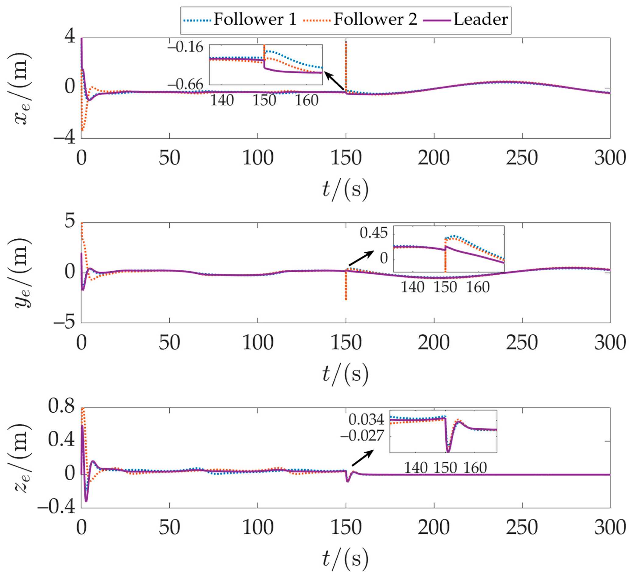
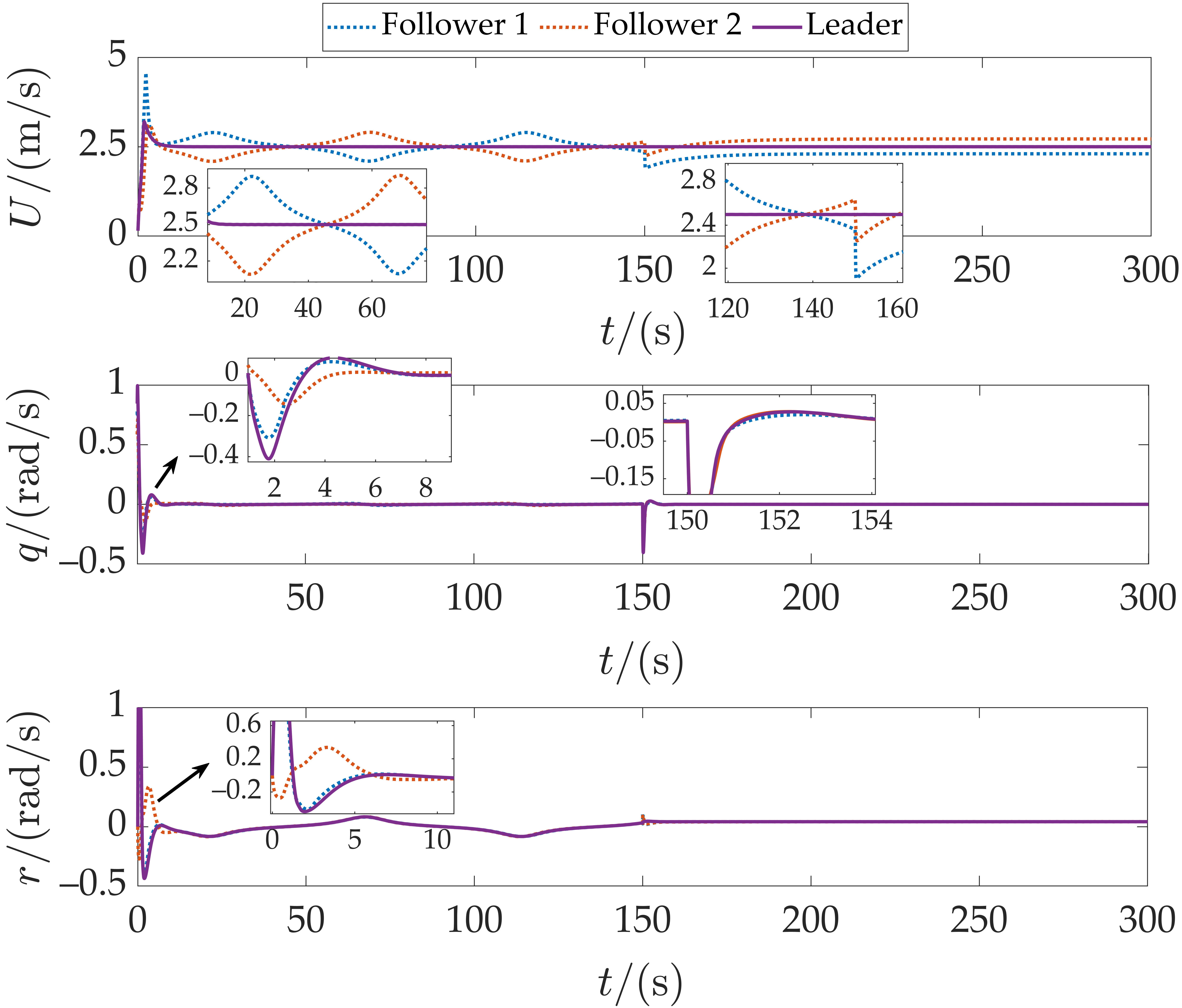
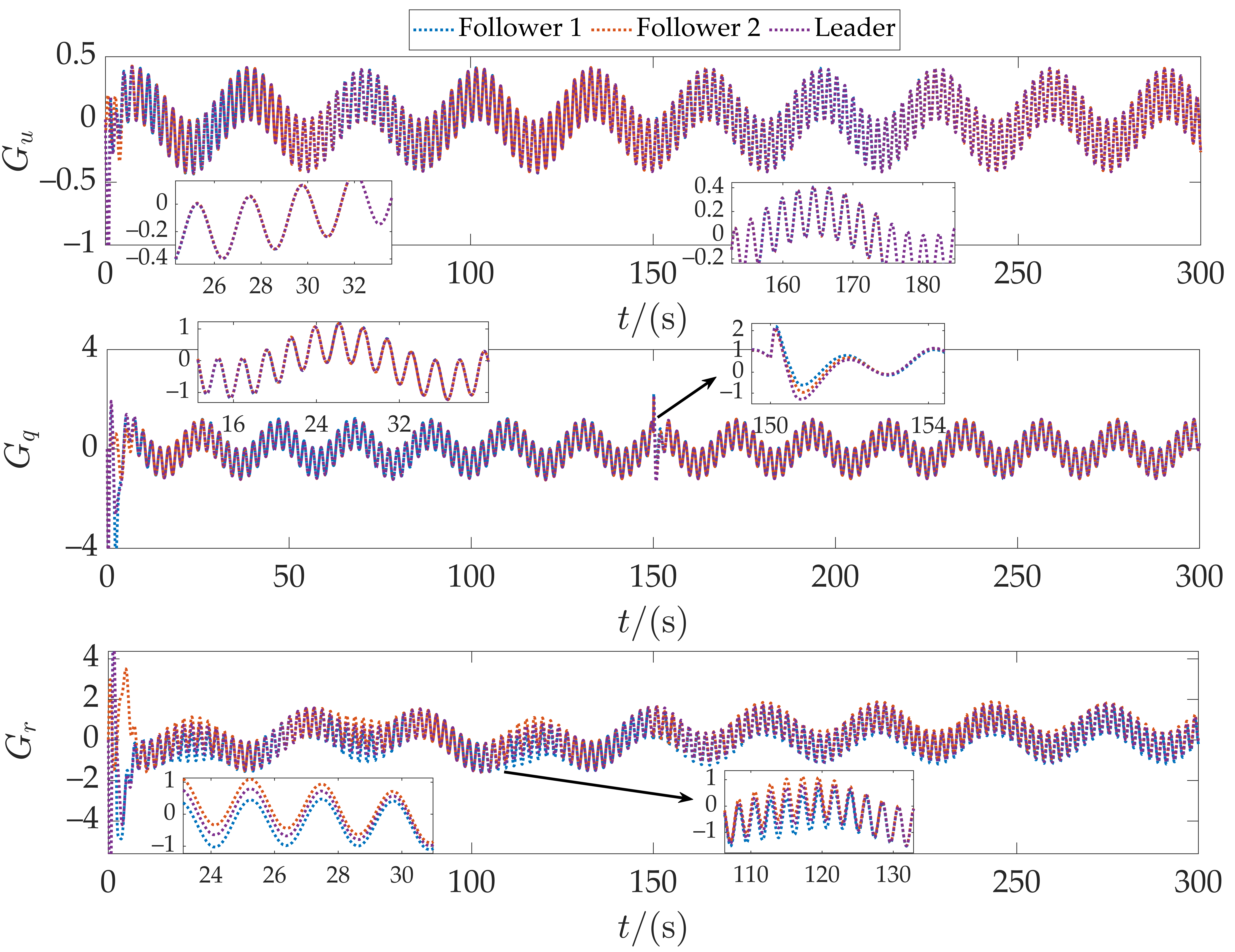
5.2. Case 2: AUV Formation Change and Maintenance

This case study aims to verify the proposed formation control method. Three underactuated AUVs are simulated to perform the following cooperative tasks:

Phase 1 (0–150 s): Dive along a spatial S-shaped path and maintain a straight formation.

Phase 2 (after 150 s): Switch to a circular path at a constant depth and reorganize into a triangular formation.

The reference path parameter equations for the leader AUV are as follows:

$$\begin{array}{cc}\left\{\begin{array}{c}{x}_{l,f}\left(s\right)=3s_l\hfill \\ y_{l,f}\left(s\right)=30\sin \left(0.1s_l\right)\hfill \\ z_{l,f}\left(s\right)=-0.5s_l\hfill \end{array}\right.\hfill & \hfill t\le 150\\ \left\{\begin{array}{c}{x}_{l,f}\left(s\right)=x_{l,\mathrm{mid}}+60\sin \left(s_l-s_{l,\mathrm{mid}}+{\psi }_{l,f,\mathrm{mid}}\right)-60\sin \left({\psi }_{l,f,\mathrm{mid}}\right)\hfill \\ y_{l,f}\left(s\right)=y_{l,\mathrm{mid}}-60\cos \left(s_l-s_{l,\mathrm{mid}}+{\psi }_{l,f,\mathrm{mid}}\right)+60\cos \left({\psi }_{l,f,\mathrm{mid}}\right)\hfill \\ z_{l,f}\left(s\right)=z_{l,\mathrm{mid}}\hfill \end{array}\right.\hfill & \hfill t>150\end{array}$$

(42)

where $x_{l,\mathrm{mid}}$, $y_{l,\mathrm{mid}}$, and $z_{l,\mathrm{mid}}$ represent the position at the 150th second. $s_{l,\mathrm{mid}}$ and ${\psi }_{l,f,\mathrm{mid}}$ represent the values of $s_l$ and ${\psi }_{l,f}$ at the 150th second, respectively.

The initial formation vectors of the AUV are ${\iota }_1={\left[0,5,0\right]}^{\mathrm{T}}$, ${\iota }_2={\left[0,-5,0\right]}^{\mathrm{T}}$, and the formation vectors after 150 s are ${\iota }_1={\left[-5,5,0\right]}^{\mathrm{T}}$, ${\iota }_2={\left[-5,-5,0\right]}^{\mathrm{T}}$. The initial bit state of the leader is ${\left[x_l\left(0\right),y_l\left(0\right),z_l\left(0\right),{\theta }_l\left(0\right),{\psi }_l\left(0\right)\right]}^{\mathrm{T}}={\left[5,2,0,0,0\right]}^{\mathrm{T}}$, and the initial velocity is ${\left[u_l\left(0\right),v_l\left(0\right),w_l\left(0\right),q_l\left(0\right),r_l\left(0\right)\right]}^{\mathrm{T}}={\left[0.15,0,0,0,0\right]}^{\mathrm{T}}$. The initial bit state of the two followers is ${\left[0,5,0,0,0\right]}^{\mathrm{T}}$, ${\left[5,5,0,0,0\right]}^{\mathrm{T}}$, and the initial velocity is ${\left[0.15,0,0,0,0\right]}^{\mathrm{T}}$. The forward speed of the formation as a whole is $U_{l,d}=2.5 \mathrm{m}/\mathrm{s}$. The constant current is the same as in Case 1. The environmental disturbance is set as follows:

$$\left\{\begin{array}{l}{\tau }_{du}=15\sin \left(1.5t\right)\cos \left(1.3t\right)\\ {\tau }_{dq}=10\sin \left(1.5t\right)\cos \left(1.2t\right) \\ {\tau }_{dr}=12\sin \left(1.3t\right)\cos \left(1.5t\right)\end{array}\right.$$

(43)

Figure 9 illustrates the formation movement paths of three AUVs, with several positions of the AUVs marked at the same time. It can be seen that the formation remains stable during both the straight-line and triangular formation stages. The designed controller ensures that the AUVs quickly converge to the reference path and maintain the formation stably, unaffected by their initial positions. The tracking error results are shown in Figure 10. Followers 1 and 2 are initially far from their reference paths, resulting in tracking errors that are significantly greater than those of the leader at the beginning. When switching from a spatial S-curve to a circular constant depth path, the curvature discontinuity of the desired path causes a temporary increase in the tracking error. Thanks to the path-following controller, the errors of all AUVs converge quickly and eventually stabilize at the same level.

Figure 11 compares the speeds of the followers and the leader. Due to the different generalized positions of each AUV, their longitudinal speeds vary. During Phase 1 (S-shaped curve, 0–150 s), the speeds of the two followers exhibit symmetrical fluctuations. This is because, at the curve bends, their angular velocities are consistent, but their curvature radii differ, resulting in differences in longitudinal speed (which must be lower or higher than the leader’s speed). In Phase 2 (circular path, after 150 s), all AUVs have the same angular velocity, and their longitudinal velocities are distributed in parallel according to their respective motion radii. The AUVs can maintain the desired formation, demonstrating that the formation coordination controller can effectively form and maintain a formation with multiple AUVs. Figure 12 shows the disturbance estimation performance of the three AUVs, indicating that the overall disturbance estimation performance is good. However, brief instability occurs at the instant when the path and formation are switched simultaneously at 150 s.

In summary, the simulation results verified the effectiveness of the controller. Under the control of the controller, the leader was able to quickly and stably follow the desired path, and the followers were also able to quickly reach the desired formation position. The three AUVs were able to achieve and stably maintain the specified formation.

6. Conclusions

This paper proposes a control method that integrates a fractional-order sliding mode observer and a cooperative control strategy for the path-following of underactuated AUVs in complex marine environments. The designed fractional-order sliding mode observer enhances the response performance to high-frequency disturbances through fractional calculus. Meanwhile, it effectively reduces sliding mode chattering using a double-power convergence law and improves the estimation accuracy of unknown disturbances, as well as system robustness via an adaptive gain mechanism. The proposed cooperative control strategy achieves formation consistency control with low communication overhead. This is achieved by setting independent reference points for each AUV and employing a path arc length parameter negotiation mechanism. For the speed adjustment problem, a proposed speed adjustment method based on the hyperbolic tangent function is designed, which effectively improves the system response speed and convergence performance. Numerical simulation results verified that this method has good path-following accuracy and formation maintenance capabilities in both constant sea currents and strong disturbance environments, demonstrating strong adaptability and robustness. Future work will focus on further optimizing the control algorithm and conducting experimental studies in open water to validate the engineering feasibility of the proposed method. In this way, it is anticipated that this research will provide theoretical support for the collaborative operation capabilities of AUVs in complex marine environments, thereby advancing the application of underwater multi-agent systems in fields such as marine exploration and resource development.

References

1. He, L.; Xie, M.; Zhang, Y. A Review of Path Following, Trajectory Tracking, and Formation Control for Autonomous Underwater Vehicles. Drones 2025, 9, 286. [Google Scholar] [CrossRef]
2. Wynn, R.B.; Huvenne, V.A.I.; Le Bas, T.P.; Murton, B.J.; Connelly, D.P.; Bett, B.J.; Ruhl, H.A.; Morris, K.J.; Peakall, J.; Parsons, D.R.; et al. Autonomous Underwater Vehicles (AUVs): Their Past, Present and Future Contributions to the Advancement of Marine Geoscience. Mar. Geol. 2014, 352, 451–468. [Google Scholar] [CrossRef]
3. Salazar, R.; Campos, A.; Fuentes, V.; Abdelkefi, A. A Review on the Modeling, Materials, and Actuators of Aquatic Unmanned Vehicles. Ocean Eng. 2019, 172, 257–285. [Google Scholar] [CrossRef]
4. Yang, Y.; Xiao, Y.; Li, T. A Survey of Autonomous Underwater Vehicle Formation: Performance, Formation Control, and Communication Capability. IEEE Commun. Surv. Tutor. 2021, 23, 815–841. [Google Scholar] [CrossRef]
5. Li, Z.; Min, G.; Ren, P.; Luo, C.; Zhao, L.; Luo, C. Ubiquitous and Robust UxV Networks: Overviews, Solutions, Challenges, and Opportunities. IEEE Netw. 2024, 38, 26–34. [Google Scholar] [CrossRef]
6. Yan, J.; Guan, X.; Yang, X.; Chen, C.; Luo, X. A Survey on Integration Design of Localization, Communication, and Control for Underwater Acoustic Sensor Networks. IEEE Internet Things J. 2025, 12, 6300–6324. [Google Scholar] [CrossRef]
7. Li, J.; Yuan, R.; Zhang, H. Research on multiple AUVs formation control algorithm based on leader-follower method. Chin. J. Sci. Instrum. 2019, 40, 237–246. [Google Scholar] [CrossRef]
8. Yang, E.; Gu, D. Nonlinear Formation-Keeping and Mooring Control of Multiple Autonomous Underwater Vehicles. IEEE/ASME Trans. Mechatron. 2007, 12, 164–178. [Google Scholar] [CrossRef]
9. Bian, J.; Xiang, J. Three-Dimensional Coordination Control for Multiple Autonomous Underwater Vehicles. IEEE Access 2019, 7, 63913–63920. [Google Scholar] [CrossRef]
10. Wang, J.; Wang, C.; Wei, Y.; Zhang, C. Sliding Mode Based Neural Adaptive Formation Control of Underactuated AUVs with Leader-Follower Strategy. Appl. Ocean Res. 2020, 94, 101971. [Google Scholar] [CrossRef]
11. Cui, R.; Sam Ge, S.; Voon Ee How, B.; Sang Choo, Y. Leader–Follower Formation Control of Underactuated Autonomous Underwater Vehicles. Ocean Eng. 2010, 37, 1491–1502. [Google Scholar] [CrossRef]
12. Millán, P.; Orihuela, L.; Jurado, I.; Rubio, F.R. Formation Control of Autonomous Underwater Vehicles Subject to Communication Delays. IEEE Trans. Control Syst. Technol. 2014, 22, 770–777. [Google Scholar] [CrossRef]
13. Park, B.S. Adaptive Formation Control of Underactuated Autonomous Underwater Vehicles. Ocean Eng. 2015, 96, 1–7. [Google Scholar] [CrossRef]
14. Yu, X. Research on Consensus Based Underwater Multi-Agent Formation Control. Master’s Thesis, Xi’an University of Technology, Xi’an, China, 2024. [Google Scholar]
15. Yan, T.; Xu, Z.; Yang, S.X. Consensus Formation Tracking for Multiple AUV Systems Using Distributed Bioinspired Sliding Mode Control. IEEE Trans. Intell. Veh. 2023, 8, 1081–1092. [Google Scholar] [CrossRef]
16. Xiang, X. Research on Path Following and Coordinated Control for Second-Order Nonholonomic AUVs. Ph.D. Thesis, Huazhong University of Science and Technology, Wuhan, China, 2010. [Google Scholar]
17. Zhang, X.; Zhou, L.; Xing, W.; Yao, S. Formation consensus control of multi-AUV system with switching topology. J. Harbin Eng. Univ. 2023, 44, 587–593. [Google Scholar]
18. Lewis, M.A.; Tan, K.-H. High Precision Formation Control of Mobile Robots Using Virtual Structures. Auton. Robot. 1997, 4, 387–403. [Google Scholar] [CrossRef]
19. Chen, Y.-L.; Ma, X.-W.; Bai, G.-Q.; Sha, Y.; Liu, J. Multi-Autonomous Underwater Vehicle Formation Control and Cluster Search Using a Fusion Control Strategy at Complex Underwater Environment. Ocean Eng. 2020, 216, 108048. [Google Scholar] [CrossRef]
20. Balch, T.; Arkin, R.C. Behavior-Based Formation Control for Multirobot Teams. IEEE Trans. Robot. Autom. 1998, 14, 926–939. [Google Scholar] [CrossRef]
21. Xu, P. Behavior-Based Formation Control of Multi-AUV. Master’s Thesis, Shanghai Jiao Tong University, Shanghai, China, 2013. [Google Scholar]
22. Wang, Q.; He, B.; Zhang, Y.; Yu, F.; Huang, X.; Yang, R. An Autonomous Cooperative System of Multi-AUV for Underwater Targets Detection and Localization. Eng. Appl. Artif. Intell. 2023, 121, 105907. [Google Scholar] [CrossRef]
23. He, L.; Zhang, Y.; Fan, G.; Liu, Y.; Wang, X.; Yuan, Z. Three-Dimensional Path Following Control of Underactuated AUV Based on Nonlinear Disturbance Observer and Adaptive Line-of-Sight Guidance. IEEE Access 2024, 12, 83911–83924. [Google Scholar] [CrossRef]
24. He, L.; Zhang, Y.; Li, S.; Li, B.; Yuan, Z. Three-Dimensional Path Following Control for Underactuated AUV Based on Ocean Current Observer. Drones 2024, 8, 672. [Google Scholar] [CrossRef]
25. Xia, Y.; Xu, K.; Li, Y.; Xu, G.; Xiang, X. Improved Line-of-Sight Trajectory Tracking Control of under-Actuated AUV Subjects to Ocean Currents and Input Saturation. Ocean Eng. 2019, 174, 14–30. [Google Scholar] [CrossRef]
26. Ali, N.; Tawiah, I.; Zhang, W. Finite-Time Extended State Observer Based Nonsingular Fast Terminal Sliding Mode Control of Autonomous Underwater Vehicles. Ocean Eng. 2020, 218, 108179. [Google Scholar] [CrossRef]
27. Ding, Z.; Wang, H.; Sun, Y.; Qin, H. Adaptive Prescribed Performance Second-Order Sliding Mode Tracking Control of Autonomous Underwater Vehicle Using Neural Network-Based Disturbance Observer. Ocean Eng. 2022, 260, 111939. [Google Scholar] [CrossRef]
28. Luo, W.; Liu, S. Disturbance Observer Based Nonsingular Fast Terminal Sliding Mode Control of Underactuated AUV. Ocean Eng. 2023, 279, 114553. [Google Scholar] [CrossRef]
29. Rong, S.; Wang, H.; Li, H.; Sun, W.; Gu, Q.; Lei, J. Performance-Guaranteed Fractional-Order Sliding Mode Control for Underactuated Autonomous Underwater Vehicle Trajectory Tracking with a Disturbance Observer. Ocean Eng. 2022, 263, 112330. [Google Scholar] [CrossRef]
30. Wang, J.; Shao, C.; Chen, X.; Chen, Y. Fractional-Order DOB-Sliding Mode Control for a Class of Noncommensurate Fractional-Order Systems with Mismatched Disturbances. Math. Meth. Appl. Sci. 2021, 44, 8228–8242. [Google Scholar] [CrossRef]
31. Wang, J.; Shao, C.; Chen, Y.-Q. Fractional Order Sliding Mode Control via Disturbance Observer for a Class of Fractional Order Systems with Mismatched Disturbance. Mechatronics 2018, 53, 8–19. [Google Scholar] [CrossRef]
32. Sun, G.; Wu, L.; Kuang, Z.; Ma, Z.; Liu, J. Practical Tracking Control of Linear Motor via Fractional-Order Sliding Mode. Automatica 2018, 94, 221–235. [Google Scholar] [CrossRef]
33. Yang, Z.; Ding, Q.; Sun, X.; Zhu, H.; Lu, C. Fractional-Order Sliding Mode Control for a Bearingless Induction Motor Based on Improved Load Torque Observer. J. Frankl. Inst. 2021, 358, 3701–3725. [Google Scholar] [CrossRef]
34. Dou, B.; Yue, X. Disturbance Observer-Based Fractional-Order Sliding Mode Control for Free-Floating Space Manipulator with Disturbance. Aerosp. Sci. Technol. 2023, 132, 108061. [Google Scholar] [CrossRef]
35. Li, W.; Qin, K.; Li, G.; Shi, M.; Zhang, X. Robust Bipartite Tracking Consensus of Multi-Agent Systems via Neural Network Combined with Extended High-Gain Observer. ISA Tran. 2023, 136, 31–45. [Google Scholar] [CrossRef] [PubMed]
36. Meng, X.; Jiang, B.; Karimi, H.R.; Gao, C. An Event-Triggered Mechanism to Observer-Based Sliding Mode Control of Fractional-Order Uncertain Switched Systems. ISA Trans. 2023, 135, 115–129. [Google Scholar] [CrossRef] [PubMed]
37. Guha, D.; Roy, P.K.; Banerjee, S. Adaptive Fractional-Order Sliding-Mode Disturbance Observer-Based Robust Theoretical Frequency Controller Applied to Hybrid Wind–Diesel Power System. ISA Trans. 2023, 133, 160–183. [Google Scholar] [CrossRef] [PubMed]
38. Fei, J.; Wang, Z.; Fang, Y. Self-Evolving Recurrent Chebyshev Fuzzy Neural Sliding Mode Control for Active Power Filter. IEEE Trans. Industr. Inform. 2023, 19, 2729–2739. [Google Scholar] [CrossRef]
39. Liang, B.; Zheng, S.; Ahn, C.K.; Liu, F. Adaptive Fuzzy Control for Fractional-Order Interconnected Systems With Unknown Control Directions. IEEE Trans. Fuzzy Syst. 2022, 30, 75–87. [Google Scholar] [CrossRef]
40. Fossen, T.I. Handbook of Marine Craft Hydrodynamics and Motion Control; Wiley: Hoboken, NJ, USA, 2021; ISBN 978-1-119-57505-4. [Google Scholar]
41. Caharija, W.; Pettersen, K.Y.; Bibuli, M.; Calado, P.; Zereik, E.; Braga, J.; Gravdahl, J.T.; Sørensen, A.J.; Milovanović, M.; Bruzzone, G. Integral Line-of-Sight Guidance and Control of Underactuated Marine Vehicles: Theory, Simulations, and Experiments. IEEE Trans. Control Syst. Technol. 2016, 24, 1623–1642. [Google Scholar] [CrossRef]
42. Fossen, T.I.; Lekkas, A.M. Direct and Indirect Adaptive Integral Line-of-Sight Path-Following Controllers for Marine Craft Exposed to Ocean Currents. Int. J. Adapt. Control Signal Process. 2017, 31, 445–463. [Google Scholar] [CrossRef]
43. Monje, C.A.; Chen, Y.; Vinagre, B.M.; Xue, D.; Feliu, V. Advances in Industrial Control. In Fractional-Order Systems and Controls; Springer: London, UK, 2010; ISBN 978-1-84996-334-3. [Google Scholar]
44. Bian, X.; Mu, C.; Yan, Z. Coordinated control for multi-UUV formation motion on a set of given paths. J. Harbin Inst. Technol. 2013, 45, 106–111. [Google Scholar]
45. He, L.; Zhang, Y.; Liu, Y.; Bai, C.; Li, L. Backstepping Sliding Mode Control for Path Following of Underactuated AUV Affected by Ocean Currents. In Proceedings of the 2024 IEEE International Conference on Unmanned Systems (ICUS), Nanjing, China, 18–20 October 2024; pp. 858–864. [Google Scholar]
Figure 1. Schematic diagram of three-dimensional path-following.
Fractalfract 09 00465 g001
Figure 2. Following control principle block diagram.
Fractalfract 09 00465 g002
Figure 3. Schematic diagram of formation control.
Fractalfract 09 00465 g003
Figure 4. Path-following in Case 1.
Fractalfract 09 00465 g004
Figure 5. Position-following error in Case 1.
Fractalfract 09 00465 g005
Figure 6. Comparison of speeds in Case 1.
Fractalfract 09 00465 g006
Figure 7. Disturbance estimation situation in Case 1. (a) Proposed method. (b) Method 1. (c) Method 2.
Fractalfract 09 00465 g007
Figure 8. Comparison of angles in Case 1.
Fractalfract 09 00465 g008
Figure 9. Formation-following situation. (a) Three-dimensional following situation (b) x-y plane projection following situation.
Fractalfract 09 00465 g009
Figure 10. Position-following error in Case 2.
Fractalfract 09 00465 g010
Figure 11. Comparison of speeds in Case 2.
Fractalfract 09 00465 g011
Figure 12. Disturbance estimation situation in Case 2.
Fractalfract 09 00465 g012
Disclaimer/Publisher’s Note: The statements, opinions and data contained in all publications are solely those of the individual author(s) and contributor(s) and not of MDPI and/or the editor(s). MDPI and/or the editor(s) disclaim responsibility for any injury to people or property resulting from any ideas, methods, instructions or products referred to in the content.