Fractional Calculus for Neutrosophic-Valued Functions and Its Application in an Inventory Lot-Sizing Problem

Abstract

Past experiences and memory significantly contribute to self-learning and improved decision-making. These can assist decision-makers in refining their strategies for better outcomes. Fractional calculus is a tool that captures a system’s memory or past experience through its repeating patterns. In the realm of uncertainty, neutrosophic set theory demonstrates greater suitability, as it independently assesses membership, non-membership, and indeterminacy. In this article, we aim to extend the theory further by introducing fractional calculus for neutrosophic-valued functions. The proposed method is applied to an economic lot-sizing problem. Numerical simulations of the lot-sizing model suggest that strong memory employment with a memory index of 0.1 can lead to an increase in average profit in memory-independent phenomena with a memory index of 1 by approximately 44% to 49%. Additionally, the neutrosophic environment yields superior profitability results compared to both precise and imprecise settings. The synergy of fractional-order dynamics and neutrosophic uncertainty modeling paves the way for enhanced decision-making in complex, ambiguous environments.

1. Introduction

The concept of “memory” holds significant importance across a wide range of situations, including those involving physical phenomena and the processes involved in making decisions. The choices made by managers concerning demand forecasting, price setting, and purchasing trends, along with customer emotions, are inevitably shaped by the accumulated experiences of those crafting the strategies. A mathematical model can be highly beneficial when examining physical events by utilizing a variety of mathematical techniques, allowing for a comprehensive understanding that closely approximates real-world situations and happenings. In this situation, the theoretical framework of fractional calculus (FC) emerged as a highly suitable and effective approach of said situation [1,2]. In ordinary derivatives, which measure how a function changes over time using integer orders, there is no mechanism to incorporate memory or retain information about past states. Consequently, ordinary calculus does not capture dynamic memory effects and is limited in its ability to reflect a system’s complete historical behavior. By contrast, the fractional derivative (FD) considers the rate of change as being shaped by all points across a given time span, with the fractional order serving as an indicator of the system’s memory retention [3,4,5,6]. It can take into account the past data leading up to the current moment or project forward from the present into future scenarios [7]. Numerous scholars [8,9] have demonstrated profound investigations into memory processes by employing the mathematical relationships inherent in FC. To demonstrate the memory effect within the context of an inventory control, the researchers propose that the rate of inventory level is expressed as a fractional value [10]. In this framework, the specific order of the FD serves as an indicator of the memory influence, and this type of derivative is called memory-dependent derivatives [11]. As the fractional order drops, it indicates stronger memory effects on the system. The system becomes less memory dependent as the fractional order nears one. Various studies on memory effect criteria in fractional-order derivatives or integrals have emerged in inventory control theory.

Developing inventory models and making managerial decisions in real-world management and applied sciences inevitably involves uncertainty. Ambiguous data can reduce decision-making precision, leading to uncertain or unpredictable conclusions. Various approaches address uncertainty—probability theory considers likelihood, fuzzy sets [12] handle belongingness, and intuitionistic fuzzy sets [13] incorporate both belongingness and non-belongingness. However, indeterminacy is also crucial. To capture this, Smarandache [14,15] introduced neutrosophic logic, which includes indeterminacy along with belongingness and non-belongingness. The key distinction of neutrosophic sets lies in explicitly including indeterminacy as an independent component, enabling a more refined representation of incomplete or vague information. This enhances their utility in fields like decision making and control theory, where uncertainty is common. For example, in predicting a reasonable selling price, three cases may arise: ‘To what extent the price is reasonable (truth)’, ‘To what extent it is unreasonable (falsity)’, and ‘Uncertainty about its reasonableness (indeterminacy)’. This underscores the significance of neutrosophic numbers. The neutrosophic number can be represented by $\left\{(\xi ;T\left(\xi \right),I\left(\xi \right), F\left(\xi \right):\xi \in X\right\}$, where $T\left(\xi \right)$, $I\left(\xi \right)$, and $F\left(\xi \right)$ are represented the degree of belongingness, indetermination, and non-belongingness, respectively, of $\xi$ to the neutrosophic set. This idea can be valuable in the context of inventory management, especially the economic order quantity (EOQ) model, where forecasting demand and determining the best pricing strategies involve uncertainties stemming from unpredictable factors. Inspired by the above inferences, the authors explored an introductory study, guided by these research questions:

• What might serve as an appropriate mathematical framework for addressing the inventory management problem when accounting for memory effects within a neutrosophic imprecise environment?
• How does memory influence inventory control strategies, particularly when price and environmental sustainability are represented as uncertain neutrosophic numbers?
• How might one articulate the mathematical structure of FC when it is situated within an environment characterized by neutrosophic uncertainty?

These research questions guided a review of the literature on fractional calculus, fuzzy logic, fuzzy-valued fractional calculus, and neutrosophic-valued calculus. A summary follows in subsequent subsections.

The paper is organized as follows: a detailed literature survey on the related topics, research gaps, and novelties of our study is presented in Section 2. Section 3 presents preliminaries on neutrosophic numbers and Riemann–Liouville and Caputo fractional differentiability. Section 4 introduces the fractional calculus theory for neutrosophic-valued functions through the Riemann–Liouville fractional integral. Section 5 covers the Riemann–Liouville fractional derivative, while Section 6 discusses the Caputo fractional derivative from the perspective of the gH-Hukuhara derivative. Section 7 applies the theory analytically to a green lot-sizing inventory model under memory and neutrosophic uncertainty. Section 8 numerically illustrates the proposed model from a managerial perspective, and Section 9 presents concluding remarks and future research directions.

2. Literature Review

This section provides a concise theoretical overview of fractional calculus, fuzzy fractional calculus, and neutrosophic calculus, along with their applications in inventory modeling.

2.1. The Literature of Fractional Calculus and Lot-Sizing Problem

Fractional calculus (FC) is an area of study that generates considerable excitement within today’s mathematical research community, with roots stretching far back into history. The core concept and understanding of what constitutes an FD have evolved significantly since it was first introduced (Das [16], Jumarie [17]). A Fractional Differential Equation (FDE) is a mathematical concept in which the traditional integer orders of a differential equation are substituted with fractional values, introducing a non-whole number order to the derivatives involved (see Kilbas et al. [18], Magin [19]). While the fundamental concept continues to develop, the investigators have yet to offer a tangible understanding of the FD’s nature. This mathematical tool possesses the remarkable ability to retain memories of previous inputs, using them to forecast the current output value—a characteristic that was later recognized as one of its most significant and useful physical interpretations (see Tarasov and Tarasova [20]). Several studies focusing on the memory effect criteria of fractional-order derivatives or integrals have been introduced within inventory control theory. For instance, Das and Roy [21] introduced the notion of FC in an inventory problem in the sense of generalization and showed that classical order models can be treated as the particular case of generalized fractional order model. Pakhira and co-authors discussed memory concerning different types of inventory models by adding various factors like the quadratic-time-dependent demand rate [22], linear-time-dependent demand with shortage [23], price-dependent demand [24], complete backlogged shortage policy [25], partial backlogged shortage policy [26,27], and time-varying holding cost [28] through the Caputo and Riemann–Liouville derivative and integration. Rahaman et al. [29] explored the role of memory effects within Economic Production Quantity (EPQ) models, examining scenarios both with and without product deterioration. Their findings highlighted that the traditional EPQ framework represents a specific instance of the broader, more generalized fractional EPQ model. Given the intricate characteristics of this approach, Rahaman et al. [30] later enhanced the EPQ model that accounts for deterioration by applying the artificial bee colony algorithm to optimize its performance. Jana and Das [31] demonstrated that the presence of a long-memory effect could prove advantageous for a company when formulating policies, as opposed to relying on systems with short-term or no memory retention. In a separate study, Rahaman et al. [32] crafted a fractional-order approach to inventory control, incorporating a demand influenced by both pricing and available stock levels. Meanwhile, Kumar et al. [33] constructed a fractional-order EOQ model that accounted for demand varying over time, alongside factors like reliability and promotional efforts. Their work explored an optimized structure for inventory management aimed at yielding the most effective decision-making outcomes. Additionally, Singh and Jain [34] investigated a demand function influenced by memory and price sensitivity to determine the best inventory strategies for items that do not deteriorate immediately. Jana et al. [35] presented a memory effect inventory model for deteriorating items using completely backlogged shortages policy. Recently, Jain et al. [36] explored how memory influences a production inventory system, taking into account an imperfect manufacturing setup and demand that varies with price. They also incorporated a rework process to address defective units. Their findings indicated that factoring memory into the inventory framework enhances the company’s overall profitability.

2.2. The Literature on Fuzzy Fractional Calculus

Agarwal et al. [37] first introduced fuzzy uncertainty in FDE and proposed the solution process through RL fractional differentiability based on the Hukuhara difference. Allahviranloo et al. [38] presented fractional RL H-differentiability of a fuzzy-valued function, which is the generalization of the fractional RL derivative using Hukuhara difference. Salahshour et al. [39] discussed the Fuzzy Fractional Differential Equation (FuFDE) using a fuzzy Laplace transform method, where the fuzzy fractional derivative (FuFD) is based on RL Hukuhara difference. Then, the solution strategy of a FuFDE under the generalized fuzzy Caputo derivative was studied by Allahviranloo et al. [40]. Mazandarani and Kamyad [41] investigated the fuzzy fractional initial value problem based on the Caputo-type FuFD with a modified fractional Euler method. A fuzzy fractional dynamical system was investigated by Najariyan and Zhao [42] through granular FuFD and the integration of RL and the Caputo method. Following this, a series of additional theoretical developments (Hoa et al. [43], Allahviranloo and Ghanbari [44], Al-Smadi et al. [45], Haq et al. [46], Wang et al. [47]) were explored within this research field, each offering unique viewpoints. Several researchers have utilized the FuFDE approach to formulate and analyze various types of inventory control models, particularly the EOQ and EPQ models. Their work has provided valuable insights and practical implications for industrial managers aiming to optimize inventory decisions under uncertainty. Notable contributions in this area can be found in the studies conducted by Rahaman et al. [48,49], Pakhira et al. [50], and Momena et al. [51]. In the current study, we expand the framework of neutrosophic-valued FC into a broader and more comprehensive context. Therefore, in the next subsection, we provide a thorough and detailed review of the recent existing literature concerning neutrosophic numbers and functions.

2.3. The Literature on Neutrosophic Calculus

Smarandache [52] first proposed the idea of a neutrosophic derivative within the framework of neutrosophic theory, building upon and extending the principles of the fuzzy derivative. Meanwhile, Son et al. [53] presented an innovative interpretation of the neutrosophic derivative, which they termed the granular derivative, and outlined the essential conditions that must be met for this derivative to apply to functions with neutrosophic values. In a different approach, Moi et al. [54,55] developed an alternative concept called the generalized neutrosophic derivative, employing this formulation to explore and analyze a second-order boundary value problem within the neutrosophic context. Sumathi and Priya [56] and Sumathi and Sweety [57] explored the concept of an NDE through the use of a parametric approach to represent neutrosophic numbers in their respective studies. Parikh et al. [58] elaborated the process of solving a first-order linear non-homogeneous fuzzy differential equation within the framework of a neutrosophic setting. Momena et al. [59] established the existence and uniqueness condition for solving the neutrosophic differential equation. Haque et al. [60] presented a generalized neutrosophic Laplace transform method for solving NDE based on the generalized neutrosophic derivative. Narzary and Basumatary [61] defined the n-th order derivative of neutrosophic real function and established the existence and uniqueness to solve the n-th order NDE.

Numerous scholars have applied neutrosophic logic across diverse domains such as control theory and decision-making processes; however, the application of Neutrosophic Differential Equations (NDEs) remains largely underexplored in addressing uncertainties within inventory control challenges. For instance, Pal and Chakraborty [62], Mondal et al. [63], Mohanta et al. [64], and Rahaman et al. [65,66] introduced various inventory frameworks, including the EOQ and Economic Production Quantity (EPQ) models, utilizing the NDE methodology to tackle such issues.

2.4. Research Gaps and Motivations

After analyzing a brief literature survey, the following research reasons motivated the authors to write this article:

• Neutrosophic uncertainty mathematically models uncertain data by separately evaluating membership, non-membership, and indeterminacy within intervals. This approach supports various applications in mathematical modeling and optimization for decision-making scenarios.
• Neutrosophic-valued calculus is key for dynamic models with neutrosophic uncertainty. Few studies explore this area.
• Fractional calculus improves on Newtonian calculus by capturing non-local, memory-dependent dynamics more effectively.
• The dynamic memory model, influenced by neutrosophic uncertainty, requires neutrosophic fractional calculus.
• So far, no research has identified the theory of fractional calculus for neutrosophic-valued functions.

2.5. Contribution and Novelties of This Paper

Considering the gaps drawn above, the significant contributions are presented as follows:

• The Riemann–Liouville definition of the fractional integral for neutrosophic-valued functions is introduced.
• Both the Riemann–Liouville and Caputo-given approaches to derivative in the neutrosophic uncertain arena are used to present the fractional differential calculus for neutrosophic-valued function.
• In addition, as a fitting outcome of the suggested theory, an economic lot-sizing model is examined under memory affection and neutrosophic uncertain phenomena.

Furthermore, the proposed theory has distinguished characteristics with a novel extension FC for neutrosophic-valued functions that integrates memory effects with the expressive capabilities of neutrosophic logic. It is worth mentioning that Riemann and Caputo defined fractional derivatives and integration possess system memory as physically significant. On the other hand, uncertainty regarding data and decision processes can be described by fuzzy, intuitionistic fuzzy, and neutrosophic environments. Fuzzy set and logic are celebrated tools in research domains of decision making and optimization, which incorporate the notion of vagueness in a moderate expressive manner through membership value. Intuitionistic fuzzy comes to depict vagueness and hesitance, together incorporating the concepts of membership and non-membership functions, and is a highly expressive approach to analyzing risk regarding financial deals. The most expressive mathematical structure is provided by neutrosophic theory for depicting the involvement of incomplete, inconsistent, and indeterminate information such as systems with conflicting data. At this stage, we assume a decision phenomenon where memory and uncertainty co-exist. Such phenomena necessitates the FC under uncertainty. In this regard, fuzzy fractional calculus has a vast literature on theoretical advancements and applications depicting vagueness and memory simultaneously. Intuitionistic fuzzy fractional calculus associates hesitation along with the existing feature of the decision phenomena. Fractional calculus for neutrosophic-valued function can be utilized for paradoxical modelling of economic and sociological phenomena that incorporates memory, indeterminacy, contradiction, and paraconsistency altogether. There is no such specific study on FC for neutrosophic-valued function and its economic implications in the existing literature. This research introduces a powerful mathematical framework that merges the long-memory characteristics of FC with the indeterminate modeling capabilities of neutrosophic sets. The resulting approach opens new avenues for analyzing and optimizing dynamic systems embedded in uncertainty, contradiction, and incomplete information, with particular promise for supply chain, economic, and engineering applications.

3. Mathematical Preliminaries

Definition 1.

A fuzzy set $\tilde{\mathcal{B}}$ in a universe of discourse $X$ is characterized as $\tilde{\mathcal{B}}=\left\{<\xi , {\mu }_{\mathcal{B}}\left(\xi \right)>:\xi \in X\right\}$, where ${\mu }_{\mathcal{B}}:X\to [0, 1]$ is a membership function, which assigns to each element $\xi \in X$ to a real number ${\mu }_{\mathcal{B}}\left(\xi \right)$ representing the degree of membership of $\xi$ in set $\tilde{\mathcal{B}}$.

Note: The value ${\mu }_{\mathcal{B}}\left(\xi \right)=0$ means that $\xi$ is not a member of $\tilde{\mathcal{B}}$, ${\mu }_{\mathcal{B}}\left(\xi \right)=1$ means that $\xi$ is a full member, and intermediate values represent partial membership. This concept generalizes the classical notion of a set, which can be seen as a special case where the membership function takes only binary values 0 and 1.

Definition 2.

The $\zeta$-cut of a fuzzy set $\tilde{\mathcal{B}}$, denoted by ${\tilde{\mathcal{B}}}_{\zeta }$, for a given $\zeta \in \left[0, 1\right]$, is the crisp subset of $X$ defined as

$${\tilde{\mathcal{B}}}_{\zeta }=\left\{\xi \in X:{\mu }_{\mathcal{B}}\left(\xi \right)\ge \zeta \right\}$$

Note: If ${\tilde{\mathcal{B}}}_{\zeta }$ is a convex fuzzy set, then its $\zeta$-cut can be represented as ${\tilde{\mathcal{B}}}_{\zeta }=\left[{\mathcal{B}}_1\left(\zeta \right),{\mathcal{B}}_2\left(\zeta \right)\right]$, where ${\mathcal{B}}_1\left(\zeta \right)=\mathit{inf}\left\{\xi \in X:{\mu }_{\mathcal{B}}\left(\xi \right)\ge \zeta \right\}$ and ${\mathcal{B}}_2\left(\zeta \right)=\mathit{sup}\left\{\xi \in X:{\mu }_{\mathcal{B}}\left(\xi \right)\ge \zeta \right\}$. Here, $\zeta$ is not a membership value of a particular element, but it represents a threshold or level of membership.

Definition 3 ([67]).

Suppose that $X$ is the universal set. A neutrosophic set $\tilde{\mathcal{B}}$ on $X$ is identified as $\tilde{\mathcal{B}}=\left\{<\xi , T_{\mathcal{B}}\left(\xi \right), I_{\mathcal{B}}\left(\xi \right), F_{\mathcal{B}}\left(\xi \right)>:\xi \in X\right\}$, where $T_{\mathcal{B}}\left(\xi \right)$, $I_{\mathcal{B}}\left(\xi \right)$, and $F_{\mathcal{B}}\left(\xi \right) :X\to [0, 1]$ signify the truthiness, indetermination, and falseness membership functions, respectively, of the component $\xi$ in $\tilde{\mathcal{B}}$ sustaining the relation $0\le T_{\mathcal{B}}\left(\xi \right)+I_{\mathcal{B}}\left(\xi \right)+F_{\mathcal{B}}\left(\xi \right)\le 3$.

Definition 4 ([67]).

The $\left(\zeta ,\eta ,\theta \right)$-cut of a neutrosophic number $\tilde{\mathcal{B}}$ on $X$ is defined as ${\tilde{\mathcal{B}}}_{\left(\zeta ,\eta ,\theta \right)}=\left\{〈T_{\mathcal{B}}\left(\xi \right), I_{\mathcal{B}}\left(\xi \right), F_{\mathcal{B}}\left(\xi \right)〉\right. :\xi \in X, T_{\mathcal{B}}\left(\xi \right)\ge \zeta , I_{\mathcal{B}}\left(\xi \right)\le \eta , \left.F_{\mathcal{B}}\left(\xi \right)\le \theta \right\},$ where $\zeta , \eta \theta$ are in $[0, 1]$.

Note: If $\tilde{\mathcal{B}}$ is a neut-convex neutrosophic set, then its $\left(\zeta ,\eta ,\theta \right)$-cut can be obtained as $\tilde{\mathcal{B}}=⟨\left[{\mathcal{B}}_1\left(\zeta \right),{\mathcal{B}}_2\left(\zeta \right)\right];\left[{\mathcal{B}}_1\left(\eta \right),{\mathcal{B}}_2\left(\eta \right)\right];\left[{\mathcal{B}}_1\left(\theta \right),{\mathcal{B}}_2\left(\theta \right)\right]⟩$, where ${\mathcal{B}}_1\left(\zeta \right)=\inf \left\{\xi \in X:T_{\mathcal{B}}\left(\xi \right)\ge \zeta \right\}$, ${\mathcal{B}}_2\left(\zeta \right)=\sup \left\{\xi \in X:{\mu }_{\mathcal{B}}\left(\xi \right)\ge \zeta \right\}$, ${\mathcal{B}}_1\left(\eta \right)=\inf \left\{\xi \in X:I_{\mathcal{B}}\left(\xi \right)\le \eta \right\}$, ${\mathcal{B}}_2\left(\eta \right)=\sup \left\{\xi \in X:I_{\mathcal{B}}\left(\xi \right)\le \eta \right\}$, ${\mathcal{B}}_1\left(\theta \right)=\inf \left\{\xi \in X:F_{\mathcal{B}}\left(\xi \right)\le \theta \right\}$ and ${\mathcal{B}}_2\left(\theta \right)=\sup \left\{\xi \in X:F_{\mathcal{B}}\left(\xi \right)\le \theta \right\}$. Here, $\zeta$, $\eta$, and $\theta$, respectively, represent the truthiness, indetermination, and falseness membership threshold. Thus, in the parametric representation of a neutrosophic set, if the indeterminacy threshold is eliminated by setting $\eta =0$, and the falsity threshold is defined as the complement of the truth parameter, i.e., $\theta =1-\zeta$, then the representation effectively reduces to that of a fuzzy representation.

Definition 5 ([67]).

A neutrosophic set $\tilde{\mathcal{B}}$ is said to be a neutrosophic number if it is defined on the universal set of real number and sustaining the following conditions:

• $ℬ$ is neut-normal, i.e., there exists points in ${\xi }_0$, ${\xi }_1$, and ${\xi }_2$ in $\mathbb{R}$ for which $T_{\mathcal{B}}\left({\xi }_0\right)=1$, $I_{\mathcal{B}}\left({\xi }_1\right)=0$ and $F_{\mathcal{B}}\left({\xi }_2\right)=0$.
• $\tilde{\mathcal{B}}$ is neut-convex, i.e., for any ${\xi }_1$ and ${\xi }_2$ of $\mathbb{R}$ and $\lambda \in [0,1]$; $T_{\mathcal{B}}$, $I_{\mathcal{B}}$, and $F_{\mathcal{B}}$ satisfy the following:

  $$T_{\mathcal{B}}\left(\lambda {\xi }_1+\left(1-\lambda \right){\xi }_2\right)\ge \mathit{min}\left\{T_{\mathcal{B}}\left({\xi }_1\right), T_{\mathcal{B}}\left({\xi }_2\right)\right\}$$

  $$I_{\mathcal{B}}\left(\lambda {\xi }_1+\left(1-\lambda \right){\xi }_2\right)\le \mathit{max}\left\{I_{\mathcal{B}}\left({\xi }_1\right), I_{\mathcal{B}}\left({\xi }_2\right)\right\}$$

  $$F_{\mathcal{B}}\left(\lambda {\xi }_1+\left(1-\lambda \right){\xi }_2\right)\le \mathit{max}\left\{F_{\mathcal{B}}\left({\xi }_1\right), F_{\mathcal{B}}\left({\xi }_2\right)\right\}$$

Note: There exist various types of neutrosophic numbers, including triangular neutrosophic numbers, trapezoidal neutrosophic numbers, etc., each designed to represent uncertainty and indeterminacy in different forms. The set of all such neutrosophic numbers is collectively denoted by $\mathcal{N}$, representing the complete class of neutrosophic numbers used in this study.

Definition 6 ([67]).

A single valued trapezoidal neutrosophic number of type-1 ${\tilde{\mathcal{B}}}_{TpN}$ is a special type of neutrosophic set defined on the set of real number $\mathbb{R}$ with the following truthiness, indetermination, and falseness membership functions:

$$T_{\mathcal{B}}\left(\xi \right)=\left\{\begin{array}{c}{\displaystyle \frac{\xi -i_1}{i_2-i_1}} when i_1\le \xi <i_2\\ 1 when i_2\le \xi \le i_3\\ {\displaystyle \frac{i_4-\xi }{i_4-i_3}} when i_3<\xi \le i_4\\ 0 otherwise\end{array}\right., I_{\mathcal{B}}\left(\xi \right)=\left\{\begin{array}{c}{\displaystyle \frac{k_2-\xi }{k_2-k_1}} when k_1\le \xi <k_2\\ 0 when k_2\le \xi \le k_3\\ {\displaystyle \frac{\xi -k_3 }{k_4-k_3}} when k_3<\xi \le k_4\\ 1 otherwise\end{array}\right., \mathrm{and}$$

$$F_{\mathcal{B}}\left(\xi \right)=\left\{\begin{array}{c}{\displaystyle \frac{l_2-\xi }{l_2-l_1}} when l_1\le \xi <l_2\\ 0 when l_2\le \xi \le l_3\\ {\displaystyle \frac{\xi -l_3}{l_4-l_3}} when l_3<\xi \le l_4\\ 1 otherwise\end{array}\right.$$

with $0\le T_{\mathcal{B}}\left(\xi \right)+I_{\mathcal{B}}\left(\xi \right)+F_{\mathcal{B}}\left(\xi \right)\le 3$ and it is denoted as ${\tilde{\mathcal{B}}}_{TpN}=⟨\left[i_1,i_2,i_3,i_4\right],\left[k_1,k_2,k_3,k_4\right],\left[l_1,l_2,l_3,l_4\right]⟩$.

Note: (i) The behavior of the membership functions associated with the above neutrosophic number ${\tilde{\mathcal{B}}}_{TpN}$ is characterized by distinct trends over specific subintervals. The truthiness membership function $T_{\mathcal{B}}\left(\xi \right)$ exhibits a linear increase over the interval $\left[i_1, i_2\right]$, remains constant throughout $\left[i_2, i_3\right]$, and then decreases over $\left[i_3, i_4\right]$. In contrast, the indeterminacy membership function $I_{\mathcal{B}}\left(\xi \right)$ decreases linearly over $\left[k_1, k_2\right]$, remains constant in the interval $\left[k_2, k_3\right]$, and increases linearly over $[k_3, k_4]$. A similar trend is observed for the falsity membership function $F_{\mathcal{B}}\left(\xi \right)$, which decreases linearly in $[l_1, l_2]$, remains constant in [$l_2, l_3]$, and increases linearly over the interval $[l_3, l_4]$.

(ii) The $\left(\zeta ,\eta ,\theta \right)$-cut of the single valued neutrosophic number of type-1 defined in definition 3.6 is obtained as $\tilde{\mathcal{B}}=⟨\left[{\mathcal{B}}_1\left(\zeta \right),{\mathcal{B}}_2\left(\zeta \right)\right];\left[{\mathcal{B}}_1\left(\eta \right),{\mathcal{B}}_2\left(\eta \right)\right];\left[{\mathcal{B}}_1\left(\theta \right),{\mathcal{B}}_2\left(\theta \right)\right]⟩$, where ${\mathcal{B}}_1\left(\zeta \right)=i_1+\zeta (i_2-i_1)$, ${\mathcal{B}}_2\left(\zeta \right)=i_4-\zeta (i_4-i_3)$, ${\mathcal{B}}_1\left(\eta \right)=k_2-\eta (k_2-k_1)$, ${\mathcal{B}}_2\left(\eta \right)=k_3+\eta (k_4-k_3)$, ${\mathcal{B}}_1\left(\theta \right)=l_2-\theta (l_2-l_1)$, and ${\mathcal{B}}_2\left(\theta \right)=l_3+\eta (l_4-l_3)$.

Definition 7 ([67]).

A single valued trapezoidal neutrosophic number ${\tilde{\mathcal{B}}}_{TpN}$ is a special type of neutrosophic set defined on the set of real number $\mathbb{R}$. It is characterized by three membership functions: the truthiness-membership function $T_{\mathcal{B}}:\mathbb{R}\to \left[0,{\rho }_{\mathcal{B}}\right]$, indetermination-membership function $I_{\mathcal{B}}:\mathbb{R}\to \left[{\sigma }_{\mathcal{B}},1\right]$, and falseness-membership function $F_{\mathcal{B}}:\mathbb{R}\to \left[{\tau }_{\mathcal{B}},1\right]$, which are defined as follows:

$$T_{\mathcal{B}}\left(\xi \right)=\left\{\begin{array}{c}\left({\displaystyle \frac{\xi -i_1}{i_2-i_1}}\right){\rho }_{\mathcal{B}} when i_1\le \xi <i_2\\ {\rho }_{\mathcal{B}} when i_2\le \xi \le i_3\\ \left({\displaystyle \frac{i_4-\xi }{i_4-i_3}}\right){\rho }_{\mathcal{B}} when i_3<\xi \le i_4\\ 0 otherwise\end{array}\right., I_{\mathcal{B}}\left(\xi \right)=\left\{\begin{array}{c}{\displaystyle \frac{i_2-\xi +{\sigma }_{\mathcal{B}}\left(\xi -i_1\right)}{i_2-i_1}} when i_1\le \xi <i_2\\ {\sigma }_{\mathcal{B}} when i_2\le \xi \le i_3\\ {\displaystyle \frac{\xi -k_3+{\sigma }_{\mathcal{B}}\left(i_4-\xi \right) }{i_4-i_3}} when i_3<\xi \le i_4\\ 1 otherwise\end{array}\right.,\mathit{and}$$

$$F_{\mathcal{B}}\left(\xi \right)=\left\{\begin{array}{c}{\displaystyle \frac{i_2-\xi +{\tau }_{\mathcal{B}}(\xi -i_1)}{i_2-i_1}} when i_1\le \xi <i_2\\ {\tau }_{\mathcal{B}} when i_2\le \xi \le i_3\\ {\displaystyle \frac{\xi -i_3+{\tau }_{\mathcal{B}}(i_4-\xi )}{i_4-i_3}} when i_3<\xi \le i_4\\ 1 otherwise\end{array}\right.$$

with $0\le T_{\mathcal{B}}\left(\xi \right)+I_{\mathcal{B}}\left(\xi \right)+F_{\mathcal{B}}\left(\xi \right)\le 3$, and it is denoted as ${\tilde{\mathcal{B}}}_{TpN}=⟨\left(i_1,i_2,i_3,i_4\right):{\rho }_{\mathcal{B}},{\sigma }_{\mathcal{B}},{\tau }_{\mathcal{B}}⟩$.

Definition 8 ([60]).

Let the $\left(\zeta ,\eta ,\theta \right)$-cut representation of a neutrosophic number $\tilde{\mathcal{B}}$ be ${\tilde{\mathcal{B}}}_{\left(\zeta ,\eta ,\theta \right)}=⟨\left[{\mathcal{B}}_1\left(\zeta \right),{\mathcal{B}}_2\left(\zeta \right)\right]; \left[{\mathcal{B}}_1\left(\eta \right), {\mathcal{B}}_2\left(\eta \right)\right]; \left[{\mathcal{B}}_1\left(\theta \right), {\mathcal{B}}_2\left(\theta \right)\right]⟩$. The de-neutrosophication value of $\tilde{\mathcal{B}}$ can be defined as

$$De\left(\tilde{\mathcal{B}}\right)={\displaystyle \frac{\zeta {\mathcal{B}}_1\left(\zeta \right)+\left(1-\zeta \right){\mathcal{B}}_2\left(\zeta \right)+\eta {\mathcal{B}}_1\left(\eta \right)+\left(1-\eta \right){\mathcal{B}}_2\left(\eta \right)+\theta {\mathcal{B}}_1\left(\theta \right)+(1-\theta ){\mathcal{B}}_2\left(\theta \right)}{3}}$$

where $0\le \zeta ,\eta ,\theta \le 1$.

Definition 9 ([54]).

Let $\widetilde{{\rm Y}}:\mathcal{I}\to \mathcal{N}$ be the neutrosophic-valued function defined on $\mathcal{I}$ whose $\left(\zeta ,\eta ,\theta \right)$-cut representation is $\widetilde{{\rm Y}}=⟨\left[{{\rm Y}}_1\left(\xi ;\zeta \right),{{\rm Y}}_2(\xi ;\zeta )\right];\left[{{\rm Y}}_1\left(\xi ;\eta \right),{{\rm Y}}_2(\xi ;\eta )\right]; \left[{{\rm Y}}_1\left(\xi ;\theta \right),{{\rm Y}}_2(\xi ;\theta )\right]⟩$. Then, the generalized neutrosophic derivative of type-1 of $\widetilde{{\rm Y}}\left(\xi \right)$ is defined as 

$${\widetilde{{\rm Y}}}^{\prime }\left(\xi \right)=⟨\left[{{\rm Y}}_1^{\prime }\left(\xi ;\zeta \right),{{\rm Y}}_2^{\prime }(\xi ;\zeta )\right];\left[{{\rm Y}}_1^{\prime }\left(\xi ;\eta \right),{{\rm Y}}_2^{\prime }(\xi ;\eta )\right]; \left[{{\rm Y}}_1^{\prime }\left(\xi ;\theta \right),{{\rm Y}}_2^{\prime }(\xi ;\theta )\right]⟩$$

and the generalized neutrosophic derivative of type-2 of $\widetilde{{\rm Y}}\left(\xi \right)$ is defined as 

$${\widetilde{\mathsf{{\rm Y}}}}^{\prime }\left(\mathsf{\xi }\right)=⟨\left[{\mathsf{{\rm Y}}}_2^{\prime }\left(\mathsf{\xi };\mathsf{\zeta }\right),{\mathsf{{\rm Y}}}_1^{\prime }(\mathsf{\xi };\mathsf{\zeta })\right];\left[{\mathsf{{\rm Y}}}_2^{\prime }\left(\mathsf{\xi };\mathsf{\eta }\right),{\mathsf{{\rm Y}}}_1^{\prime }(\mathsf{\xi };\mathsf{\eta })\right];\left[{\mathsf{{\rm Y}}}_2^{\prime }\left(\mathsf{\xi };\mathsf{\theta }\right),{\mathsf{{\rm Y}}}_1^{\prime }(\mathsf{\xi };\mathsf{\theta })\right]⟩$$

Definition 10 ([18]).

The left-sided Riemann–Liouville Fractional Integral (RLFI) ${}^{RL}\mathcal{I}_a^{\beta }\left({\rm Y}\left(\xi \right)\right)$ of order $\beta \left(0<\beta <1\right)$ of a continuous function ${\rm Y}:\left[a, b\right]\to \mathbb{R}$, which has a bounded derivative in $\left[a, b\right]$, is defined as 

$${}^{RL}\mathcal{I}_a^{\beta }\left({\rm Y}\left(\xi \right)\right)={\displaystyle \frac{1}{\Gamma \left(\beta \right)}}{\int }_a^{\xi }{\displaystyle \frac{{\rm Y}\left(\chi \right)}{{\left(\xi -\chi \right)}^{1-\beta }}}d\chi$$

for all, $\xi \in [a,b]$. The left-sided Riemann–Liouville fractional derivative (RLFD) ${}^{RL}\mathcal{D}_a^{\alpha }\left({\rm Y}\left(\xi \right)\right)$ of order $\alpha$ of a continuous function is 

$${}^{RL}\mathcal{D}_a^{\alpha }\left({\rm Y}\left(\xi \right)\right)={\displaystyle \frac{1}{\Gamma \left(m-\alpha \right)}}{\left({\displaystyle \frac{d}{d\xi }}\right)}^m{\int }_a^{\xi }{\displaystyle \frac{{\rm Y}\left(\chi \right)}{{\left(\xi -\chi \right)}^{\alpha +1-m}}}d\chi$$

for all, $\xi \in [a,b]$ and $0\le m-1<\alpha <m$.

Note. The fundamental distinction between the RLFD and ordinary derivative is that the RLFD of a constant value does not result in zero.

Definition 11 ([18]).

The left-sided Caputo fractional derivative (CFD) ${}^C\mathcal{D}_a^{\alpha }\left({\rm Y}\left(\xi \right)\right)$ of order $\alpha \left(0<\alpha <1\right)$ of a continuous function ${\rm Y}:\left[a, b\right]\to \mathbb{R}$, which has a bounded derivative in $\left[a, b\right]$, is defined as 

$${}^C\mathcal{D}_a^{\alpha }\left({\rm Y}\left(\xi \right)\right)={\displaystyle \frac{1}{\Gamma \left(m-\alpha \right)}}\underset{a}{\overset{\xi }{\int }}{\displaystyle \frac{1}{{\left(\xi -\chi \right)}^{\alpha +1-m}}}{\displaystyle \frac{d^m}{d{\chi }^m}}\left({\rm Y}\left(\chi \right)\right) d\chi$$

for all, $\xi \in [a,b]$ and $0\le m-1<\alpha <m$.

Note. ${}^C\mathcal{D}_a^{\alpha }\left(c\right)=0$, where $c$ is constant.

In the next three sections, the notion of the R-L fractional integral, R-L fractional derivative, and Caputo fractional derivative for the neutrosophic-valued function is introduced. The symbols that are used to define the notion of FC of the neutrosophic-valued function are presented in

Table 1. List of notations used to discuss the theoretical counterpart regarding the fractional calculus of the neutrosophic-valued function.

Notations	Explanation
$\xi$	Independent variable
$\widetilde{\mathsf{{\rm Y}}}\left(\xi \right)$	Neutrosophic-valued function of $\xi$
$\mathcal{N}$	Set of all neutrosophic number
${{\rm Y}}_1$	Lower component of the parametric representation of the neutrosophic-valued function $\widetilde{\mathsf{{\rm Y}}}\left(\xi \right)$
${{\rm Y}}_2$	Upper component of the parametric representation of the neutrosophic-valued function $\widetilde{\mathsf{{\rm Y}}}\left(\xi \right)$
$\zeta$	Truthiness membership threshold of the parametric representation of neutrosophic number/function
$\eta$	Indeterminacy membership threshold of the parametric representation of neutrosophic number/function
$\theta$	Falseness membership threshold of the parametric representation of neutrosophic number/function
$\alpha$	Order of fractional derivative
$\beta$	Order of fractional integration
$\chi$	Parameters
$s$	Laplace transform parameter $s>0$
$\mathsf{\Gamma }$	Gamma function
${\ominus }_h$	Generalized Hukuhara difference
${}^{RL}\mathcal{I}_a^{\beta }\left(\widetilde{{\rm Y}}\left(\xi \right)\right)$	R-L fractional integration of $\widetilde{\mathsf{{\rm Y}}}\left(\xi \right)$$\mathrm{of} \mathrm{order} \beta$$\mathrm{with} \mathrm{base} \mathrm{point} a>0$
${}^{RL}\mathcal{D}_a^{\alpha }\left(\widetilde{{\rm Y}}\left(\xi \right)\right)$	R-L fractional derivative of $\widetilde{\mathsf{{\rm Y}}}\left(\xi \right)$$\mathrm{of} \mathrm{order} \alpha$$\mathrm{with} \mathrm{base} \mathrm{point} a>0$
${}^C\mathcal{D}_a^{\alpha }\left(\widetilde{{\rm Y}}\left(\xi \right)\right)$	Caputo fractional derivative of $\widetilde{\mathsf{{\rm Y}}}\left(\xi \right)$$\mathrm{of} \mathrm{order} \alpha$$\mathrm{with} \mathrm{base} \mathrm{point} a>0$

.

4. R-L Fractional Integral of Neutrosophic-Valued Functions

Based on the Hukuhara difference and the original notion of RLFI in crisp case, we here presented the definition of Neutrosophic-valued Riemann–Liouville Fractional Integration (NRLFI).

Definition 12.

Let $\widetilde{{\rm Y}}:[a,b]\to \mathcal{N}$ be a Lebesgue integrable neutrosophic-valued function defined on $[a,b]$. Suppose the parametric representation of $\widetilde{{\rm Y}}\left(\xi \right)$ is given as $\widetilde{{\rm Y}}\left(\xi \right)=⟨\left[{{\rm Y}}_1\left(\xi ;\zeta \right),{{\rm Y}}_2(\xi ;\zeta )\right], \left[{{\rm Y}}_1\left(\xi ;\eta \right),{{\rm Y}}_2(\xi ;\eta )\right], \left[{{\rm Y}}_1\left(\xi ;\theta \right),{{\rm Y}}_2(\xi ;\theta )\right]⟩$; for all, $0\le \zeta , \eta , \theta \le 1$. Then, each of the real valued functions of $\widetilde{{\rm Y}}\left(\xi \right)$ is the Lebesgue integrable function defined on $[a,b]$. This indicated that, for all, $\beta \in \left(\mathrm{0,1}\right)$, all the real valued functions ${\displaystyle \frac{{{\rm Y}}_1\left(\chi ;\zeta \right)}{{\left(\xi -\chi \right)}^{1-\beta }}}$, ${\displaystyle \frac{{{\rm Y}}_2\left(\chi ;\zeta \right)}{{\left(\xi -\chi \right)}^{1-\beta }}}$, ${\displaystyle \frac{{{\rm Y}}_1\left(\chi ;\eta \right)}{{\left(\xi -\chi \right)}^{1-\beta }}}$, ${\displaystyle \frac{{{\rm Y}}_2\left(\chi ;\eta \right)}{{\left(\xi -\chi \right)}^{1-\beta }}}$, ${\displaystyle \frac{{{\rm Y}}_1\left(\chi ;\theta \right)}{{\left(\xi -\chi \right)}^{1-\beta }}}$, and ${\displaystyle \frac{{{\rm Y}}_2\left(\chi ;\theta \right)}{{\left(\xi -\chi \right)}^{1-\beta }}}$ are also Lebesgue integrable on $[a,b]$. Accordingly, ${\displaystyle \frac{\widetilde{{\rm Y}}\left(\chi \right)}{{\left(\xi -\chi \right)}^{1-\beta }}}=⟨\left[{\displaystyle \frac{{{\rm Y}}_1\left(\chi ;\zeta \right)}{{\left(\xi -\chi \right)}^{1-\beta }}}, {\displaystyle \frac{{{\rm Y}}_2\left(\chi ;\zeta \right)}{{\left(\xi -\chi \right)}^{1-\beta }}}\right],\left[{\displaystyle \frac{{{\rm Y}}_1\left(\chi ;\eta \right)}{{\left(\xi -\chi \right)}^{1-\beta }}}, {\displaystyle \frac{{{\rm Y}}_2\left(\chi ;\eta \right)}{{\left(\xi -\chi \right)}^{1-\beta }}}\right],\left[{\displaystyle \frac{{{\rm Y}}_1\left(\chi ;\theta \right)}{{\left(\xi -\chi \right)}^{1-\beta }}}, {\displaystyle \frac{{{\rm Y}}_2\left(\chi ;\theta \right)}{{\left(\xi -\chi \right)}^{1-\beta }}}\right]⟩$ is also the Lebesgue integrable neutrosophic-valued function defined on $[a,b]$. Thus, the integral 

$${\displaystyle \frac{1}{\mathsf{\Gamma }\left(\beta \right)}}{\int }_a^{\xi }{\displaystyle \frac{\widetilde{\mathsf{{\rm Y}}}\left(\chi \right)}{{\left(\xi -\chi \right)}^{1-\beta }}}d\chi$$

(1)

($\chi$ is a parameter) exists for all $\xi \in [a,b]$, and it is denoted by ${}^{RL}\mathcal{I}_a^{\beta }\left(\widetilde{{\rm Y}}\left(\xi \right)\right)$, called the NRLFI of fractional order $\beta >0$ of the neutrosophic function $\widetilde{\mathsf{{\rm Y}}}\left(\xi \right)$.

Note: In this paper, the concept of integration of the neutrosophic-valued function is explored through the framework of neutrosophic Riemann integration (Biswas et al. [68]).

Since $\widetilde{{\rm Y}}\left(\xi \right)=⟨\left[{{\rm Y}}_1\left(\xi ;\zeta \right),{{\rm Y}}_2(\xi ;\zeta )\right], \left[{{\rm Y}}_1\left(\xi ;\eta \right),{{\rm Y}}_2(\xi ;\eta )\right], \left[{{\rm Y}}_1\left(\xi ;\theta \right),{{\rm Y}}_2(\xi ;\theta )\right]⟩$, the NRLFI of the neutrosophic-valued function $\widetilde{\mathsf{{\rm Y}}}\left(\xi \right)$ can be stated through the parametric representation as follows:

$$\begin{array}{c}{}^{RL}\mathcal{I}_a^{\beta }\left(\widetilde{{\rm Y}}\left(\xi \right)\right)=\hfill \\ ⟨\left[{\displaystyle \frac{1}{\Gamma \left(\beta \right)}}{\int }_a^{\xi }{\displaystyle \frac{{{\rm Y}}_1\left(\chi ;\zeta \right)}{{\left(\xi -\chi \right)}^{1-\beta }}}d\chi ,{\displaystyle \frac{1}{\Gamma \left(\beta \right)}}{\int }_a^{\xi }{\displaystyle \frac{{{\rm Y}}_2\left(\chi ;\zeta \right)}{{\left(\xi -\chi \right)}^{1-\beta }}}d\chi \right]; \left[{\displaystyle \frac{1}{\Gamma \left(\beta \right)}}{\int }_a^{\xi }{\displaystyle \frac{{{\rm Y}}_1\left(\chi ;\eta \right)}{{\left(\xi -\chi \right)}^{1-\beta }}}d\chi ,{\displaystyle \frac{1}{\Gamma \left(\beta \right)}}{\int }_a^{\xi }{\displaystyle \frac{{{\rm Y}}_2\left(\chi ;\eta \right)}{{\left(\xi -\chi \right)}^{1-\beta }}}d\chi \right];\hfill \end{array}$$

$$\left[{\displaystyle \frac{1}{\Gamma \left(\beta \right)}}{\int }_a^{\xi }{\displaystyle \frac{{{\rm Y}}_1\left(\chi ;\theta \right)}{{\left(\xi -\chi \right)}^{1-\beta }}}d\chi ,{\displaystyle \frac{1}{\Gamma \left(\beta \right)}}{\int }_a^{\xi }{\displaystyle \frac{{{\rm Y}}_2\left(\chi ;\theta \right)}{{\left(\xi -\chi \right)}^{1-\beta }}}d\chi \right]⟩$$

$=⟨\left[{}^{RL}\mathcal{I}_a^{\beta }\left({\mathsf{{\rm Y}}}_1\left(\xi ;\zeta \right)\right),{}^{RL}\mathcal{I}_a^{\beta }\left({\mathsf{{\rm Y}}}_2\left(\xi ;\zeta \right)\right)\right];\left[{}^{RL}\mathcal{I}_a^{\beta }\left({\mathsf{{\rm Y}}}_1\left(\xi ;\eta \right)\right),{}^{RL}\mathcal{I}_a^{\beta }\left({\mathsf{{\rm Y}}}_2\left(\xi ;\eta \right)\right)\right];$ $\left[{}^{RL}\mathcal{I}_a^{\beta }\left({\mathsf{{\rm Y}}}_1\left(\xi ;\theta \right)\right),{}^{RL}\mathcal{I}_a^{\beta }\left({\mathsf{{\rm Y}}}_2\left(\xi ;\theta \right)\right)\right]⟩$ for all $0\le \zeta ,\eta ,\theta \le 1$, where ${}^{RL}\mathcal{I}_a^{\beta }\left(\mathsf{\Psi }\left(x\right)\right)={\displaystyle \frac{1}{\mathsf{\Gamma }\left(\beta \right)}}{\int }_a^{\xi }{\displaystyle \frac{\mathsf{\Psi }\left(\chi \right)}{{\left(\xi -\chi \right)}^{1-\beta }}}d\chi$ is the RLFI of order $\beta$ of the crisp valued function $\mathsf{\Psi }$.

Remarks 1.

(i) It is important to note that when $\widetilde{{\rm Y}}\left(\xi \right)$ is a crisp function, this definition corresponds to the classical RLFI of order $\beta \in \left(\mathrm{0,1}\right]$. (ii) In the specific case where $\beta =1$ and $\widetilde{{\rm Y}}\left(\xi \right)$ is a neutrosophic-valued measurable function, this formulation encompasses the standard neutrosophic integral.

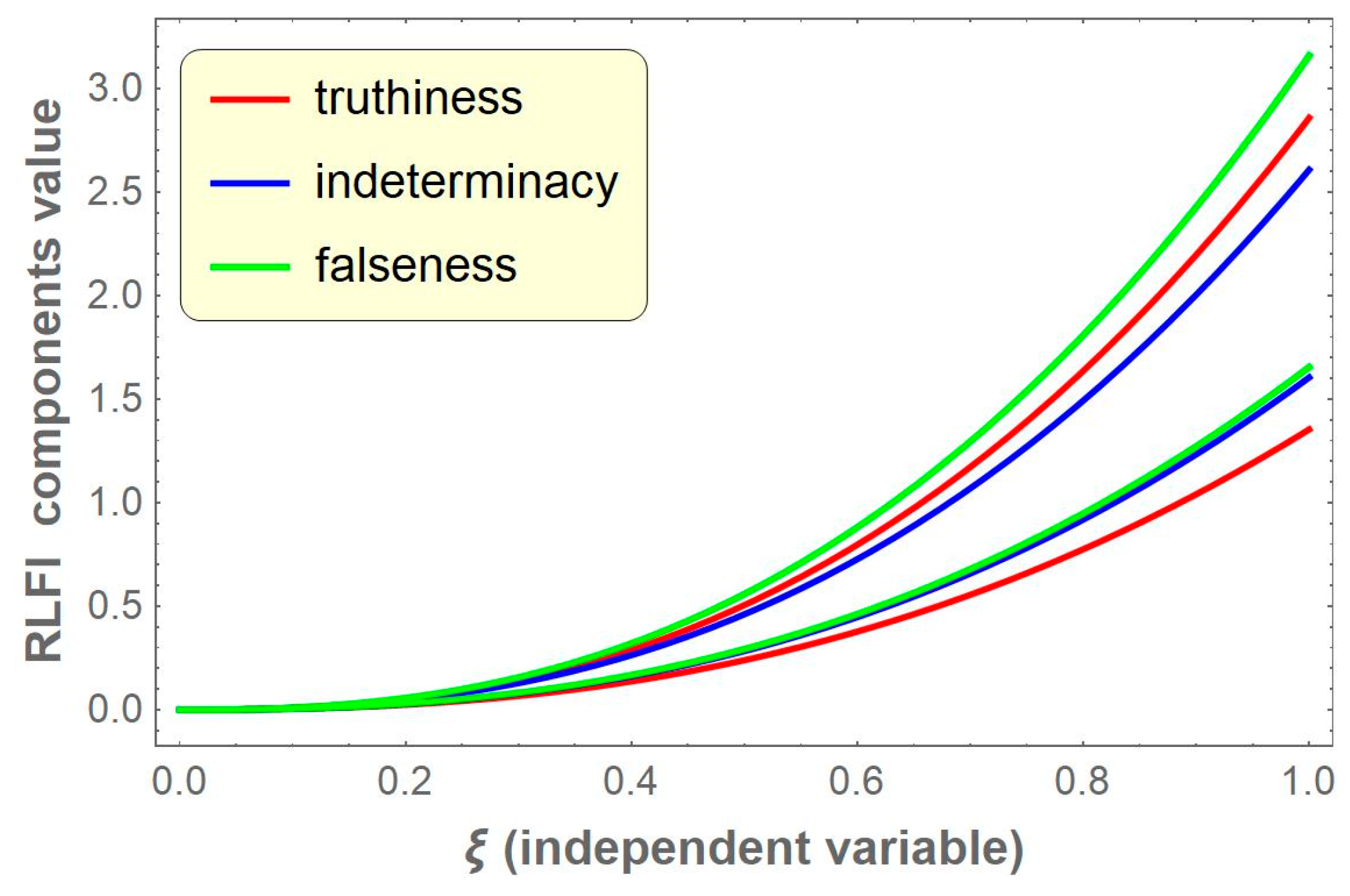
Example 1.

Suppose a neutrosophic-valued function $\widetilde{{\rm Y}}:\left[\mathrm{0,1}\right]\to \mathcal{N}$ is given as $\widetilde{{\rm Y}}\left(\xi \right)=\tilde{k}{\xi }^2$, where $\tilde{k}=〈\left(\mathrm{2,3},\mathrm{4,5}\right):\mathrm{0.8,0.4,0.2}〉$ is a single valued trapezoidal neutrosophic number. Then, the components of the $\left(\zeta ,\eta ,\theta \right)$-cut of $\widetilde{{\rm Y}}\left(\xi \right)$ are

$${{\rm Y}}_1\left(\xi ;\zeta \right)=k_1\left(\zeta \right){\xi }^2, {{\rm Y}}_2\left(\xi ;\zeta \right)=k_2\left(\zeta \right){\xi }^2$$

$${{\rm Y}}_1\left(\xi ;\eta \right)=k_1\left(\eta \right){\xi }^2, {{\rm Y}}_2\left(\xi ;\eta \right)=k_2\left(\eta \right){\xi }^2$$

$${{\rm Y}}_1\left(\xi ;\theta \right)=k_1\left(\theta \right){\xi }^2, {{\rm Y}}_2\left(\xi ;\theta \right)=k_2\left(\theta \right){\xi }^2$$

Also, the components of the $\left(\zeta ,\eta ,\theta \right)$-cut of $\tilde{k}$ are obtained as

$$k_1\left(\zeta \right)={\displaystyle \frac{8+5\zeta }{4}}, k_2\left(\zeta \right)={\displaystyle \frac{20-5\zeta }{4}}$$

$$k_1\left(\eta \right)={\displaystyle \frac{11-5\eta }{3}}, k_2\left(\eta \right)={\displaystyle \frac{10+5\eta }{3}}$$

$$k_1\left(\theta \right)={\displaystyle \frac{13-5\theta }{4}}, k_2\left(\theta \right)={\displaystyle \frac{19+5\theta }{4}}$$

where $\zeta \in \left[0, 0.8\right]$, $\eta \in \left[0.4, 1\right]$, and $\theta \in \left[\mathrm{0.2,1}\right]$. Then, the RLFI of order $\beta$ of the neutrosophic function $\widetilde{\mathsf{{\rm Y}}}\left(\xi \right)$ is

$${}^{RL}\mathcal{I}_a^{\beta }\left(\widetilde{{\rm Y}}\left(\xi \right)\right)=⟨\left[{\displaystyle \frac{\left(8+5\zeta \right)}{2\Gamma \left(\beta +3\right)}}{\xi }^{\beta +2},{\displaystyle \frac{\left(20-5\zeta \right)}{2\Gamma \left(\beta +3\right)}}{\xi }^{\beta +2}\right]; \left[{\displaystyle \frac{2\left(11-5\eta \right)}{3\Gamma \left(\beta +3\right)}}{\xi }^{\beta +2},{\displaystyle \frac{2\left(10+5\eta \right)}{3\Gamma \left(\beta +3\right)}}{\xi }^{\beta +2}\right];$$

$$\left[{\displaystyle \frac{\left(13-5\theta \right)}{2\Gamma \left(\beta +3\right)}}{\xi }^{\beta +2}, {\displaystyle \frac{\left(19+5\theta \right)}{2\Gamma \left(\beta +3\right)}}{\xi }^{\beta +2}\right]⟩$$

The six components of RL fractional integrals of the neutrosophic function $\widetilde{\mathsf{{\rm Y}}}\left(\xi \right)=\tilde{k}{\xi }^2$ are presented graphically in Figure 1 for particular fractional order $\beta =0.5$ and $\zeta =0.2$, $\eta =0.6$, and $\theta =0.4$ with respect to independent variable $\xi$. The region between red curves represents the truthiness area of the RLFI value, and, similarly, the region between the blue curves and green curves represents the indeterminacy and falseness area of RLFI value, respectively. For any given $\xi$, all six components are clearly visible in the figure.

Table 2. Numerical value of the six components of NRLFI of $\widetilde{\mathsf{{\rm Y}}}\left(\xi \right)=\tilde{k}{\xi }^2$ at order $\beta =0.5$ and $\xi =1$ for different values of $\zeta \in (0, 0.8)$, $\eta \in (0.4, 1)$, and $\theta \in \left(0.2, 1\right)$.

$\mathit{\zeta }$	${}^{\mathit{R}\mathit{L}}\mathcal{I}_0^{0.5}\left({\mathsf{{\rm Y}}}_1\left(\mathit{\xi };\mathit{\zeta }\right)\right)$	${}^{\mathit{R}\mathit{L}}\mathcal{I}_0^{0.5}\left({\mathit{{\rm Y}}}_2\left(\mathit{\xi };\mathit{\zeta }\right)\right)$	$\mathit{\eta }$	${}^{\mathit{R}\mathit{L}}\mathcal{I}_0^{0.5}\left({\mathit{{\rm Y}}}_1\left(\mathit{\xi };\mathit{\eta }\right)\right)$	${}^{\mathit{R}\mathit{L}}\mathcal{I}_0^{0.5}\left({\mathit{{\rm Y}}}_2\left(\mathit{\xi };\mathit{\eta }\right)\right)$	$\mathit{\theta }$	${}^{\mathit{R}\mathit{L}}\mathcal{I}_0^{0.5}\left({\mathit{{\rm Y}}}_1\left(\mathit{\xi };\mathit{\theta }\right)\right)$	${}^{\mathit{R}\mathit{L}}\mathcal{I}_0^{0.5}\left({\mathit{{\rm Y}}}_2\left(\mathit{\xi };\mathit{\theta }\right)\right)$
0	1.203604	3.009011	0.4	1.805407	2.407209	0.2	1.805407	3.009011
0.2	1.354055	2.858561	0.6	1.604806	2.607810	0.4	1.654956	3.159462
0.4	1.504506	2.708110	0.8	1.404205	2.808410	0.6	1.504506	3.309912
0.6	1.654956	2.557659	0.9	1.303905	2.908711	0.8	1.354055	3.460363
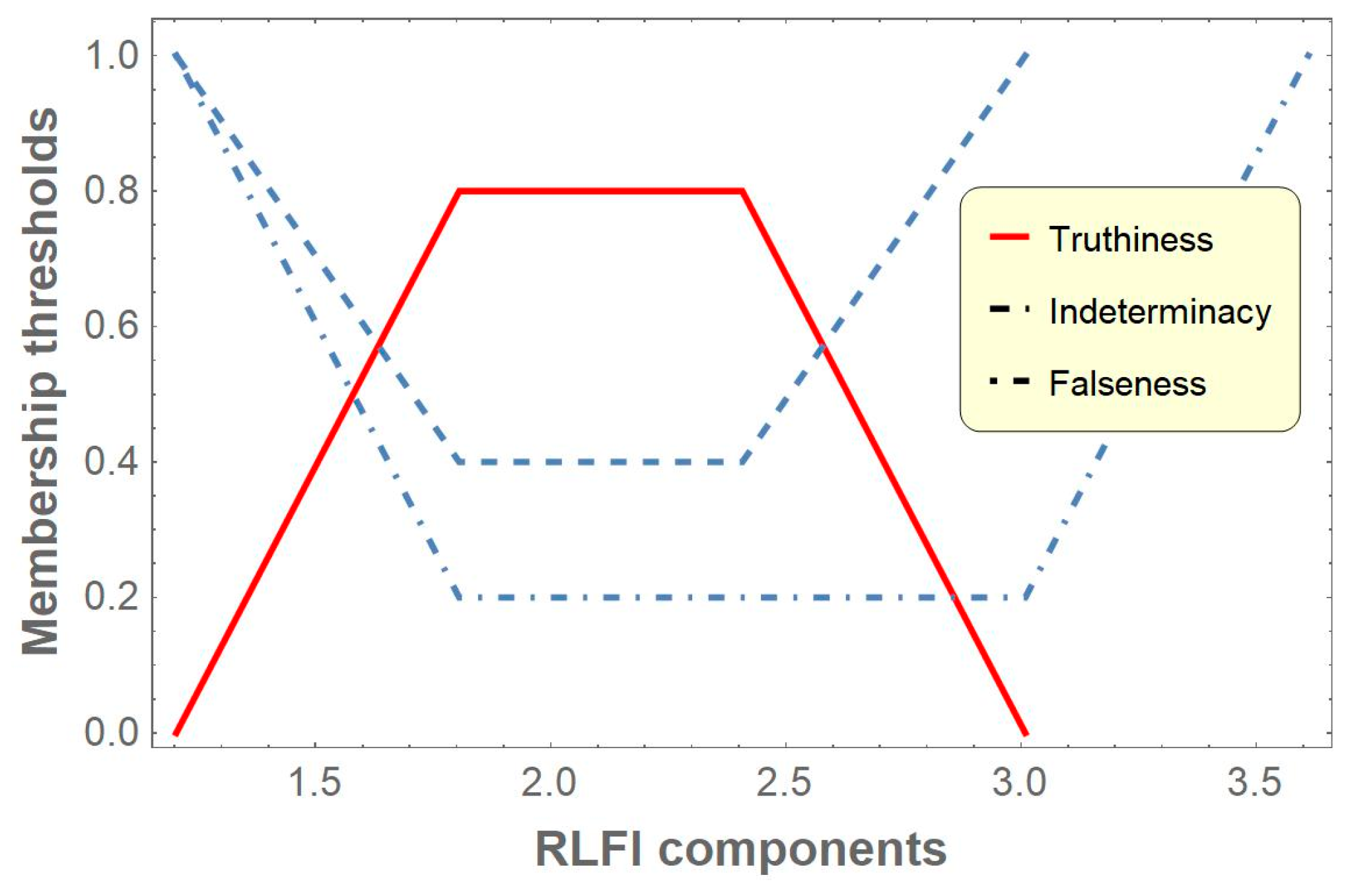
0.8	1.805407	2.407209	1.0	1.203604	3.009011	1.0	1.203604	3.610813

includes the different components of RLFI of the neutrosophic-valued function $\widetilde{\mathsf{{\rm Y}}}\left(\xi \right)=\tilde{k}{\xi }^2$ at fractional integration order $\beta =0.5$ and $\xi =1$ for different values of membership thresholds $\zeta$, $\eta$, and $\theta$. When the value of truth membership threshold $\zeta$ increases, the value of ${}^{RL}\mathcal{I}_0^{0.5}\left({\mathsf{{\rm Y}}}_1\left(\xi ;\zeta \right)\right)$ increases but ${}^{RL}\mathcal{I}_0^{0.5}\left({\mathsf{{\rm Y}}}_2\left(\xi ;\zeta \right)\right)$ decreases. Again, when the value of indeterminacy threshold $\eta$ increases, the value of ${}^{RL}\mathcal{I}_0^{0.5}\left({{\rm Y}}_1\left(\xi ;\eta \right)\right)$ decreases but ${}^{RL}\mathcal{I}_0^{0.5}\left({{\rm Y}}_1\left(\xi ;\eta \right)\right)$ increases, and the same occurs for the falseness membership threshold $\theta$. These components are presented graphically in Figure 2. Figure 2 illustrates that the RL fractional integration of $\widetilde{\mathsf{{\rm Y}}}\left(\xi \right)$ is also a trapezoidal neutrosophic number.

Lemma 1.

Let ${}^{RL}\mathcal{I}_a^{{\beta }_1}\left(\widetilde{{\rm Y}}\left(\xi \right)\right)$ and ${}^{RL}\mathcal{I}_a^{{\beta }_2}\left(\widetilde{{\rm Y}}\left(\xi \right)\right)$ be two R-L fractionals integrals of the neutrosophic-valued function $\widetilde{{\rm Y}}:\left[a, b\right]\to \mathcal{N}$ of order ${\beta }_1$ and ${\beta }_2$ respectively, where ${\beta }_1,{\beta }_2\in \left(\mathrm{0,1}\right]$ are real numbers. Then, the R-L fractional integration of $\widetilde{{\rm Y}}\left(\xi \right)$ of order ${\beta }_1+{\beta }_2$ is

$${}^{RL}\mathcal{I}_a^{{\beta }_1+{\beta }_2}\left(\widetilde{{\rm Y}}\left(\xi \right)\right)={}^{RL}\mathcal{I}_a^{{\beta }_1}\left({}^{RL}\mathcal{I}_a^{{\beta }_2}\left(\widetilde{{\rm Y}}\left(\xi \right)\right)\right)$$

provided ${\beta }_1+{\beta }_2<1$.

Proof. 

From Definition 12, the R-L fractional integration of $\widetilde{\mathsf{{\rm Y}}}\left(\xi \right)$ of order ${\beta }_1+{\beta }_2$ is

$$\begin{array}{c}{}^{RL}\mathcal{I}_a^{{\beta }_1+{\beta }_2}\left(\widetilde{\mathsf{{\rm Y}}}\left(\xi \right)\right)=\hfill \\ ⟨\left[{}^{RL}\mathcal{I}_a^{{\beta }_1+{\beta }_2}\left({\mathsf{{\rm Y}}}_1\left(\xi ;\zeta \right)\right),{}^{RL}\mathcal{I}_a^{{\beta }_1+{\beta }_2}\left({\mathsf{{\rm Y}}}_2\left(\xi ;\zeta \right)\right)\right], \left[{}^{RL}\mathcal{I}_a^{{\beta }_1+{\beta }_2}\left({\mathsf{{\rm Y}}}_1\left(\xi ;\eta \right)\right),{}^{RL}\mathcal{I}_a^{{\beta }_1+{\beta }_2}\left({\mathsf{{\rm Y}}}_2\left(\xi ;\eta \right)\right)\right],\hfill \\ \left[{}^{RL}\mathcal{I}_a^{{\beta }_1+{\beta }_2}\left({\mathsf{{\rm Y}}}_1\left(\xi ;\theta \right)\right),{}^{RL}\mathcal{I}_a^{{\beta }_1+{\beta }_2}\left({\mathsf{{\rm Y}}}_2\left(\xi ;\theta \right)\right)\right]⟩,\hfill \end{array}$$

$$\begin{array}{c}=⟨\left[{}^{RL}\mathcal{I}_a^{{\beta }_1}\left({}^{RL}\mathcal{I}_a^{{\beta }_2}\left({\mathsf{{\rm Y}}}_1\left(\xi ;\zeta \right)\right)\right),{}^{RL}\mathcal{I}_a^{{\beta }_1}\left({}^{RL}\mathcal{I}_a^{{\beta }_2}\left({\mathsf{{\rm Y}}}_2\left(\xi ;\zeta \right)\right)\right)\right], \left[{}^{RL}\mathcal{I}_a^{{\beta }_1}\left({}^{RL}\mathcal{I}_a^{{\beta }_2}\left({\mathsf{{\rm Y}}}_1\left(\xi ;\eta \right)\right)\right), \right.\hfill \\ \left.{}^{RL}\mathcal{I}_a^{{\beta }_1}\left({}^{RL}\mathcal{I}_a^{{\beta }_2}\left({\mathsf{{\rm Y}}}_2\left(\xi ;\eta \right)\right)\right)\right], \left[{}^{RL}\mathcal{I}_a^{{\beta }_1}\left({}^{RL}\mathcal{I}_a^{{\beta }_2}\left({\mathsf{{\rm Y}}}_1\left(\xi ;\theta \right)\right)\right),{}^{RL}\mathcal{I}_a^{{\beta }_1}\left({}^{RL}\mathcal{I}_a^{{\beta }_2}\left({\mathsf{{\rm Y}}}_2\left(\xi ;\theta \right)\right)\right)\right]⟩\hfill \end{array}$$

almost everywhere on $[a,b]$, if ${\beta }_1+{\beta }_2<1$.

$$={}^{RL}\mathcal{I}_a^{{\beta }_1}\left({}^{RL}\mathcal{I}_a^{{\beta }_2}\left(\widetilde{{\rm Y}}\left(\xi \right)\right)\right).$$

□

Lemma 2.

Let ${}^{RL}\mathcal{I}_a^{\beta }\left(\widetilde{{{\rm Y}}^1}\left(\xi \right)\right)$ and ${}^{RL}\mathcal{I}_a^{\beta }\left(\widetilde{{{\rm Y}}^2}\left(\xi \right)\right)$ be two NRLFIs of order $\beta$ for the neutrosophic-valued functions $\left(\widetilde{{{\rm Y}}^1}\left(\xi \right)\right)$ and $\left(\widetilde{{{\rm Y}}^2}\left(\xi \right)\right)$, respectively. Then,

$${}^{RL}\mathcal{I}_a^{\beta }\left(\widetilde{{{\rm Y}}^1}+\widetilde{{{\rm Y}}^2}\right)\left(\xi \right)={}^{RL}\mathcal{I}_a^{\beta }\left(\widetilde{{{\rm Y}}^1}\left(\xi \right)\right)+{}^{RL}\mathcal{I}_a^{\beta }\left(\widetilde{{{\rm Y}}^2}\left(\xi \right)\right).$$

Proof. 

The proof is simple and thus omitted. □

5. R-L Fractional Derivative of Neutrosophic-Valued Functions

Based on the Hukuhara difference and the original notion of the RLFD in the crisp case, we here presented the definition of the neutrosophic-valued Riemann–Liouville fractional derivative (NRLFD).

Definition 13.

Suppose that $\widetilde{{\rm Y}}\left(\xi \right)$ is a neutrosophic-valued function that is absolutely continuous over $[a,b]$ and the parametric representation of $\widetilde{{\rm Y}}\left(\xi \right)$ is given as

$$\widetilde{{\rm Y}}\left(\xi \right)=⟨\left[{{\rm Y}}_1\left(\xi ;\zeta \right),{{\rm Y}}_2(\xi ;\zeta )\right], \left[{{\rm Y}}_1\left(\xi ;\eta \right),{{\rm Y}}_2(\xi ;\eta )\right], \left[{{\rm Y}}_1\left(\xi ;\theta \right),{{\rm Y}}_2(\xi ;\theta )\right]⟩$$

for all, $0\le \zeta ,\eta ,\theta \le 1$.

Then, each of the real valued functions of $\widetilde{\mathsf{{\rm Y}}}\left(\xi \right)$ is Lebesgue integrable defined on $[a,b]$. This indicates that, for all, $\alpha \in \left(\mathrm{0,1}\right)$, and all the real valued functions ${\displaystyle \frac{{{\rm Y}}_1\left(\chi ;\zeta \right)}{{\left(\xi -\chi \right)}^{\alpha }}}$, ${\displaystyle \frac{{{\rm Y}}_2\left(\chi ;\zeta \right)}{{\left(\xi -\chi \right)}^{\alpha }}}$, ${\displaystyle \frac{{{\rm Y}}_1\left(\chi ;\eta \right)}{{\left(\xi -\chi \right)}^{\alpha }}}$, ${\displaystyle \frac{{{\rm Y}}_2\left(\chi ;\eta \right)}{{\left(\xi -\chi \right)}^{\alpha }}}$, ${\displaystyle \frac{{{\rm Y}}_1\left(\chi ;\theta \right)}{{\left(\xi -\chi \right)}^{\alpha }}}$ and ${\displaystyle \frac{{{\rm Y}}_2\left(\chi ;\theta \right)}{{\left(\xi -\chi \right)}^{\alpha }}}$ are also Lebesgue integrable on $[a,b]$. Accordingly,

$${\displaystyle \frac{\widetilde{{\rm Y}}\left(\chi \right)}{{\left(\xi -\chi \right)}^{\alpha }}}=⟨\left[{\displaystyle \frac{{{\rm Y}}_1\left(\chi ;\zeta \right)}{{\left(\xi -\chi \right)}^{\alpha }}}, {\displaystyle \frac{{{\rm Y}}_2\left(\chi ;\zeta \right)}{{\left(\xi -\chi \right)}^{\alpha }}}\right],\left[{\displaystyle \frac{{{\rm Y}}_1\left(\chi ;\eta \right)}{{\left(\xi -\chi \right)}^{\alpha }}}, {\displaystyle \frac{{{\rm Y}}_2\left(\chi ;\eta \right)}{{\left(\xi -\chi \right)}^{\alpha }}}\right],\left[{\displaystyle \frac{{{\rm Y}}_1\left(\chi ;\theta \right)}{{\left(\xi -\chi \right)}^{\alpha }}}, {\displaystyle \frac{{{\rm Y}}_2\left(\chi ;\theta \right)}{{\left(\xi -\chi \right)}^{\alpha }}}\right]⟩$$

is also a Lebesgue integrable neutrosophic function over $[a,b]$. Thus, the NRLFI of order $1-\alpha$

$${}^{RL}\mathcal{I}_a^{1-\alpha }\left(\widetilde{{\rm Y}}\left(\xi \right)\right)={\displaystyle \frac{1}{\Gamma (1-\alpha )}}{\int }_a^{\xi }{\displaystyle \frac{\widetilde{{\rm Y}}\left(\chi \right)}{{\left(\xi -\chi \right)}^{\alpha }}}d\chi$$

exists for all $\xi \in [a,b]$. Then, its generalized neutrosophic derivative ${\displaystyle \frac{d}{d\xi }}\left({}^{RL}\mathcal{I}_a^{1-\alpha }\left(\widetilde{{\rm Y}}\left(\xi \right)\right)\right)$ is denoted as ${}^{RL}\mathcal{D}_a^{\alpha }\left(\widetilde{{\rm Y}}\left(\xi \right)\right)$, called the neutrosophic-valued Riemann–Liouville fractional derivative (NRLFD) of order $\mathsf{\alpha }>0$. Therefore,

$${}^{RL}\mathcal{D}_a^{\alpha }\left(\widetilde{{\rm Y}}\left(\xi \right)\right)={\displaystyle \frac{1}{\mathsf{\Gamma }(1-\alpha )}}{\displaystyle \frac{d}{d\xi }}\left({\int }_a^{\xi }{\displaystyle \frac{\widetilde{{\rm Y}}\left(\chi \right)}{{\left(\xi -\chi \right)}^{\alpha }}}d\chi \right)$$

If the neutrosophic-valued function $\widetilde{\mathsf{{\rm Y}}}\left(\xi \right)$ is type-1 generalized neutrosophic differentiable, then ${}^{RL}\mathcal{D}_a^{\alpha }\left(\widetilde{{\rm Y}}\left(\xi \right)\right)$ is called type-1 NRLFD of order $\alpha$, and if $\widetilde{\mathsf{{\rm Y}}}\left(\xi \right)$ is type-2 generalized neutrosophic differentiable, then ${}^{RL}\mathcal{D}_a^{\alpha }\left(\widetilde{{\rm Y}}\left(\xi \right)\right)$ is called type-2 NRLFD of order $\alpha$.

Note: The NRLFD of order $\alpha$ of $\widetilde{\mathsf{{\rm Y}}}\left(\xi \right)$ is the derivative of NRLFI of order $1-\alpha$ of $\widetilde{\mathsf{{\rm Y}}}\left(\xi \right)$, i.e.,

$${}^{RL}\mathcal{D}_a^{\alpha }\left(\widetilde{{\rm Y}}\left(\xi \right)\right)={\displaystyle \frac{d}{d\xi }}\left({}^{RL}\mathcal{I}_a^{1-\alpha }\left(\widetilde{{\rm Y}}\left(\xi \right)\right)\right)$$

Theorem 1.

Suppose $\widetilde{{\rm Y}}:\left(a,b\right)\to \mathcal{N}$ is a neutrosophic-valued function and NRLFD of $\widetilde{{\rm Y}}\left(\xi \right)$ exists for all $\xi \in \left(a,b\right)$ and its parametric form can be obtained as follows:

(i)

If $\widetilde{\mathsf{{\rm Y}}}\left(\xi \right)$ is a type-1 generalized neutrosophic differentiable function, then

$$\begin{array}{cc}\hfill {}^{RL}\mathcal{D}_a^{\alpha }\left(\widetilde{\mathsf{{\rm Y}}}\left(\xi \right)\right)=& ⟨\left[{}^{RL}\mathcal{D}_a^{\alpha }\left({\mathsf{{\rm Y}}}_1\left(\xi ;\zeta \right)\right),{}^{RL}\mathcal{D}_a^{\alpha }\left({\mathsf{{\rm Y}}}_2\left(\xi ;\zeta \right)\right)\right], \left[{}^{RL}\mathcal{D}_a^{\alpha }\left({\mathsf{{\rm Y}}}_1\left(\xi ;\eta \right)\right),{}^{RL}\mathcal{D}_a^{\alpha }\left({\mathsf{{\rm Y}}}_2\left(\xi ;\eta \right)\right)\right], \hfill \\ & \left[{}^{RL}\mathcal{D}_a^{\alpha }\left({\mathsf{{\rm Y}}}_1\left(\xi ;\theta \right)\right),{}^{RL}\mathcal{D}_a^{\alpha }\left({\mathsf{{\rm Y}}}_2\left(\xi ;\theta \right)\right)\right]⟩\hfill \end{array}$$

(ii)

If $\widetilde{\mathsf{{\rm Y}}}\left(\xi \right)$ is a type-2 generalized neutrosophic differentiable function, then

$$\begin{array}{cc}\hfill {}^{RL}\mathcal{D}_a^{\alpha }\left(\widetilde{\mathsf{{\rm Y}}}\left(\xi \right)\right)=& ⟨\left[{}^{RL}\mathcal{D}_a^{\alpha }\left({\mathsf{{\rm Y}}}_2\left(\xi ;\zeta \right)\right),{}^{RL}\mathcal{D}_a^{\alpha }\left({\mathsf{{\rm Y}}}_1\left(\xi ;\zeta \right)\right)\right], \left[{}^{RL}\mathcal{D}_a^{\alpha }\left({\mathsf{{\rm Y}}}_2\left(\xi ;\eta \right)\right),{}^{RL}\mathcal{D}_a^{\alpha }\left({\mathsf{{\rm Y}}}_1\left(\xi ;\eta \right)\right)\right], \hfill \\ & \left[{}^{RL}\mathcal{D}_a^{\alpha }\left({\mathsf{{\rm Y}}}_2\left(\xi ;\theta \right)\right),{}^{RL}\mathcal{D}_a^{\alpha }\left({\mathsf{{\rm Y}}}_1\left(\xi ;\theta \right)\right)\right]⟩\hfill \end{array}$$

where ${}^{RL}\mathcal{D}_a^{\alpha }\mathsf{\Psi }\left(\xi \right)={\displaystyle \frac{1}{\mathsf{\Gamma }(1-\alpha )}}{\displaystyle \frac{d}{d\xi }}{\int }_a^{\xi }{\displaystyle \frac{\mathsf{\Psi }\left(\chi \right)}{{\left(\xi -\chi \right)}^{\alpha }}}d\chi$ is the RLFD of order $\alpha \in \left(\mathrm{0,1}\right)$ of the crisp valued function $\mathsf{\Psi }\left(\chi \right)$ and $0\le \zeta ,\eta ,\theta \le 1$.

Proof. 

First, we assume that $\widetilde{\mathsf{{\rm Y}}}\left(\xi \right)$ is a type-1 generalized neutrosophic differentiable. Then, according to Moi et al. [54], the six components of the derivative of ${\int }_a^{\xi }{\displaystyle \frac{\widetilde{{\rm Y}}\left(\chi \right)}{{\left(\xi -\chi \right)}^{\alpha }}}d\chi$ can be obtained as

$${\displaystyle \frac{d}{d\xi }}\left({\int }_a^{\xi }{\displaystyle \frac{\widetilde{{\rm Y}}\left(\chi \right)}{{\left(\xi -\chi \right)}^{\alpha }}}d\chi \right)=⟨\begin{array}{c}\left[{\displaystyle \frac{d}{d\xi }}\left({\int }_a^{\xi }{\displaystyle \frac{{{\rm Y}}_1\left(\chi ;\zeta \right)}{{\left(\xi -\chi \right)}^{\alpha }}}ds\right), {\displaystyle \frac{d}{d\xi }}\left({\int }_a^{\xi }{\displaystyle \frac{{{\rm Y}}_2\left(\chi ;\zeta \right)}{{\left(\xi -\chi \right)}^{\alpha }}}ds\right)\right];\end{array}$$

$$\left[{\displaystyle \frac{d}{d\xi }}\left({\int }_a^{\xi }{\displaystyle \frac{{{\rm Y}}_1\left(\chi ;\eta \right)}{{\left(\xi -\chi \right)}^{\alpha }}}ds\right), {\displaystyle \frac{d}{d\xi }}\left({\int }_a^{\xi }{\displaystyle \frac{{{\rm Y}}_2\left(\chi ;\eta \right)}{{\left(\xi -\chi \right)}^{\alpha }}}ds\right)\right];\left[{\displaystyle \frac{d}{d\xi }}\left({\int }_a^{\xi }{\displaystyle \frac{{{\rm Y}}_1\left(\chi ;\theta \right)}{{\left(\xi -\chi \right)}^{\alpha }}}ds\right), {\displaystyle \frac{d}{d\xi }}\left({\int }_a^{\xi }{\displaystyle \frac{{{\rm Y}}_2\left(\chi ;\theta \right)}{{\left(\xi -\chi \right)}^{\alpha }}}ds\right)\right]⟩$$

By imposing ${\displaystyle \frac{1}{\mathsf{\Gamma }(1-\alpha )}}$ on both sides of the above expression, we get

$${\displaystyle \frac{1}{\mathsf{\Gamma }(1-\alpha )}}{\displaystyle \frac{d}{d\xi }}\left({\int }_a^{\xi }{\displaystyle \frac{\widetilde{{\rm Y}}\left(\chi \right)}{{\left(\xi -\chi \right)}^{\alpha }}}d\chi \right)=⟨\begin{array}{c}\left[{\displaystyle \frac{1}{\Gamma (1-\alpha )}}{\displaystyle \frac{d}{d\xi }}\left({\int }_a^{\xi }{\displaystyle \frac{{{\rm Y}}_1\left(\chi ;\zeta \right)}{{\left(\xi -\chi \right)}^{\alpha }}}ds\right),{\displaystyle \frac{1}{\Gamma (1-\alpha )}} {\displaystyle \frac{d}{d\xi }}\left({\int }_a^{\xi }{\displaystyle \frac{{{\rm Y}}_2\left(\chi ;\zeta \right)}{{\left(\xi -\chi \right)}^{\alpha }}}ds\right)\right];\end{array}$$

$$\begin{array}{c}\left[{\displaystyle \frac{1}{\mathsf{\Gamma }(1-\alpha )}}{\displaystyle \frac{d}{d\xi }}\left({\int }_a^{\xi }{\displaystyle \frac{{\mathsf{{\rm Y}}}_1\left(\chi ;\eta \right)}{{\left(\xi -\chi \right)}^{\alpha }}}ds\right), {\displaystyle \frac{1}{\mathsf{\Gamma }(1-\alpha )}}{\displaystyle \frac{d}{d\xi }}\left({\int }_a^{\xi }{\displaystyle \frac{{\mathsf{{\rm Y}}}_2\left(\chi ;\eta \right)}{{\left(\xi -\chi \right)}^{\alpha }}}ds\right)\right];\left[{\displaystyle \frac{1}{\mathsf{\Gamma }(1-\alpha )}}{\displaystyle \frac{d}{d\xi }}\left({\int }_a^{\xi }{\displaystyle \frac{{\mathsf{{\rm Y}}}_1\left(\chi ;\theta \right)}{{\left(\xi -\chi \right)}^{\alpha }}}ds\right), \right.\\ \left.{\displaystyle \frac{1}{\mathsf{\Gamma }(1-\alpha )}}{\displaystyle \frac{d}{d\xi }}\left({\int }_a^{\xi }{\displaystyle \frac{{\mathsf{{\rm Y}}}_2\left(\chi ;\theta \right)}{{\left(\xi -\chi \right)}^{\alpha }}}ds\right)\right]⟩\end{array}$$

By using the definition of RLFD, we get

$$\begin{array}{c}{}^{RL}\mathcal{D}_a^{\alpha }\left(\widetilde{\mathsf{{\rm Y}}}\left(\xi \right)\right)=⟨\left[{}^{RL}\mathcal{D}_a^{\alpha }\left({\mathsf{{\rm Y}}}_1\left(\xi ;\zeta \right)\right),{}^{RL}\mathcal{D}_a^{\alpha }\left({\mathsf{{\rm Y}}}_2\left(\xi ;\zeta \right)\right)\right], \left[{}^{RL}\mathcal{D}_a^{\alpha }\left({\mathsf{{\rm Y}}}_1\left(\xi ;\eta \right)\right),{}^{RL}\mathcal{D}_a^{\alpha }\left({\mathsf{{\rm Y}}}_2\left(\xi ;\eta \right)\right)\right], \\ \left[{}^{RL}\mathcal{D}_a^{\alpha }\left({\mathsf{{\rm Y}}}_1\left(\xi ;\theta \right)\right),{}^{RL}\mathcal{D}_a^{\alpha }\left({\mathsf{{\rm Y}}}_2\left(\xi ;\theta \right)\right)\right]⟩\end{array}$$

For case (ii), when $\widetilde{\mathsf{{\rm Y}}}\left(\xi \right)$ is a type-2 generalized neutrosophic differentiable, the proof can be conducted through the same approach and hence omitted. □

Lemma 3.

Suppose $\widetilde{{\rm Y}}:\left(a,b\right)\to \mathcal{N}$ is a neutrosophic-valued measurable function and $0<\alpha <1$. Then, the following expression holds almost everywhere on $\left[a, b\right]$:

(i)

$\left({}^{RL}\mathcal{D}_a^{\alpha }{}^{RL}\mathcal{I}_a^{\alpha }\widetilde{\mathsf{{\rm Y}}}\right)\left(\xi \right)=⟨\left[{\mathsf{{\rm Y}}}_1\left(\xi ;\zeta \right),{\mathsf{{\rm Y}}}_2\left(\xi ;\zeta \right)\right];\left[{\mathsf{{\rm Y}}}_1\left(\xi ;\eta \right),{\mathsf{{\rm Y}}}_2\left(\xi ;\eta \right)\right];\left[{\mathsf{{\rm Y}}}_1\left(\xi ;\theta \right),{\mathsf{{\rm Y}}}_2(\xi ;\theta )\right]⟩$ for the case of type-1 generalized neutrosophic differentiability.

(ii)

$\left({}^{RL}\mathcal{D}_a^{\alpha }{}^{RL}\mathcal{I}_a^{\alpha }\widetilde{\mathsf{{\rm Y}}}\right)\left(\xi \right)=⟨\left[{\mathsf{{\rm Y}}}_2\left(\xi ;\zeta \right),{\mathsf{{\rm Y}}}_1\left(\xi ;\zeta \right)\right];\left[{\mathsf{{\rm Y}}}_2\left(\xi ;\eta \right),{\mathsf{{\rm Y}}}_1\left(\xi ;\eta \right)\right];\left[{\mathsf{{\rm Y}}}_2\left(\xi ;\theta \right),{\mathsf{{\rm Y}}}_1(\xi ;\theta )\right]⟩$for the case of type-2 generalised neutrosophic differentiability.

Proof. 

From Definition 3 and Theorem 1 for case (i):

$$\begin{array}{cc}\hfill \left({}^{RL}\mathcal{D}_a^{\alpha }\widetilde{\mathsf{{\rm Y}}}\right)\left(\xi \right)=& ⟨\left[{\displaystyle \frac{d}{d\xi }}\left({}^{RL}\mathcal{I}_a^{1-\alpha }\left({\mathsf{{\rm Y}}}_1\left(\xi ;\zeta \right)\right)\right),{\displaystyle \frac{d}{d\xi }}\left({}^{RL}\mathcal{I}_a^{1-\alpha }\left({\mathsf{{\rm Y}}}_2\left(\xi ;\zeta \right)\right)\right)\right],[{\displaystyle \frac{d}{d\xi }}\left({}^{RL}\mathcal{I}_a^{1-\alpha }\left({\mathsf{{\rm Y}}}_1\left(\xi ;\theta \right)\right)\right), \hfill \\ & {\displaystyle \frac{d}{d\xi }}\left({}^{RL}\mathcal{I}_a^{1-\alpha }\left({\mathsf{{\rm Y}}}_2\left(\xi ;\eta \right)\right)\right)],\left[{\displaystyle \frac{d}{d\xi }}\left({}^{RL}\mathcal{I}_a^{1-\alpha }\left({\mathsf{{\rm Y}}}_1\left(\xi ;\theta \right)\right)\right), {\displaystyle \frac{d}{d\xi }}\left({}^{RL}\mathcal{I}_a^{1-\alpha }\left({\mathsf{{\rm Y}}}_2\left(\xi ;\theta \right)\right)\right)\right]⟩\hfill \end{array}$$

Consequently,

$$\begin{array}{c}\left({}^{RL}\mathcal{D}_a^{\alpha }{}^{RL}\mathcal{I}_a^{\alpha }\widetilde{\mathsf{{\rm Y}}}\right)\left(\xi \right)\hfill \\ =⟨\left[{\displaystyle \frac{d}{d\xi }}\left({}^{RL}\mathcal{I}_a^{1-\alpha }{}^{RL}\mathcal{I}_a^{\alpha }\left({\mathsf{{\rm Y}}}_1\left(\xi ;\zeta \right)\right)\right),{\displaystyle \frac{d}{d\xi }}\left({}^{RL}\mathcal{I}_a^{1-\alpha }{}^{RL}\mathcal{I}_a^{\alpha }\left({\mathsf{{\rm Y}}}_2\left(\xi ;\zeta \right)\right)\right)\right],\left[{\displaystyle \frac{d}{d\xi }}\left({}^{RL}\mathcal{I}_a^{1-\alpha }{}^{RL}\mathcal{I}_a^{\alpha }\left({\mathsf{{\rm Y}}}_1\left(\xi ;\eta \right)\right)\right), \right.\hfill \\ \left.{\displaystyle \frac{d}{d\xi }}\left({}^{RL}\mathcal{I}_a^{1-\alpha }{}^{RL}\mathcal{I}_a^{\alpha }\left({\mathsf{{\rm Y}}}_2\left(\xi ;\eta \right)\right)\right)\right],\left[{\displaystyle \frac{d}{d\xi }}\left({}^{RL}\mathcal{I}_a^{1-\alpha }{}^{RL}\mathcal{I}_a^{\alpha }\left({\mathsf{{\rm Y}}}_1\left(\xi ;\theta \right)\right)\right), {\displaystyle \frac{d}{d\xi }}\left({}^{RL}\mathcal{I}_a^{1-\alpha }{}^{RL}\mathcal{I}_a^{\alpha }\left({\mathsf{{\rm Y}}}_2\left(\xi ;\theta \right)\right)\right)\right]⟩\hfill \end{array}$$

$$=⟨\left[{{\rm Y}}_1\left(\xi ;\zeta \right),{{\rm Y}}_2\left(\xi ;\zeta \right)\right], \left[{{\rm Y}}_1\left(\xi ;\eta \right),{{\rm Y}}_2\left(\xi ;\eta \right)\right], \left[{{\rm Y}}_1\left(\xi ;\theta \right),{{\rm Y}}_2(\xi ;\theta )\right]⟩$$

For case (ii), when $\widetilde{\mathsf{{\rm Y}}}\left(\xi \right)$ is type-2 generalised neutrosophic differentiability, the proof can be conducted through the same approach, and this completes the proof.

Lemma 4.

Suppose $\widetilde{{\rm Y}}\left(\xi \right)$ is a neutrosophic-valued measurable and $p$-integrable function, $1\le p<\infty$ and ${}^{RL}\mathcal{I}_a^{\alpha }\left(\widetilde{{\rm Y}}\left(\xi \right)\right)$ is an absolutely continuous function on $\left[a, b\right]$. Then, for $0<\alpha <1$

(i)

$\left({}^{RL}\mathcal{I}_a^{\alpha }{}^{RL}\mathcal{D}_a^{\alpha }\widetilde{\mathsf{{\rm Y}}}\right)\left(\xi \right)=\widetilde{\mathsf{{\rm Y}}}\left(\xi \right){\ominus }_h{\displaystyle \frac{{\left(\xi -a\right)}^{\alpha -1}}{\mathsf{\Gamma }\left(\mathsf{\alpha }\right)}}{}^{RL}\mathcal{I}_a^{1-\alpha }\left(\widetilde{\mathsf{{\rm Y}}}\left(\xi \right)\right)$

for the case of type-1 generalized neutrosophic differentiability.

(ii)

$\left({}^{RL}\mathcal{I}_a^{\alpha }{}^{RL}\mathcal{D}_a^{\alpha }\widetilde{\mathsf{{\rm Y}}}\right)\left(\xi \right)=-\left({\displaystyle \frac{{\left(\xi -a\right)}^{\alpha -1}}{\mathsf{\Gamma }\left(\mathsf{\alpha }\right)}}{}^{RL}\mathcal{I}_a^{1-\alpha }\left(\widetilde{\mathsf{{\rm Y}}}\left(\xi \right)\right)\right){\ominus }_h\left(-\widetilde{\mathsf{{\rm Y}}}\left(\xi \right)\right)$

for the case of type-2 generalized neutrosophic differentiability.

Proof. 

From Definition 12 of R-L fractional integration, we obtain

$$\begin{array}{c}\left({}^{RL}\mathcal{I}_a^{\alpha }{}^{RL}\mathcal{D}_a^{\alpha }\widetilde{{\rm Y}}\right)\left(\xi \right)=⟨\left[{\displaystyle \frac{d}{d\xi }}{\displaystyle \frac{1}{\Gamma \left(\alpha +1\right)}}{\int }_0^{\xi }{\left(\xi -\chi \right)}^{\alpha }{}^{RL}\mathcal{D}_a^{\alpha }\left({{\rm Y}}_1\left(\xi ;\zeta \right)\right)d\chi ,{\displaystyle \frac{d}{d\xi }}{\displaystyle \frac{1}{\Gamma \left(\alpha +1\right)}}{\int }_0^{\xi }{\left(\xi -\chi \right)}^{\alpha }{}^{RL}\mathcal{D}_a^{\alpha }\left({{\rm Y}}_2\left(\xi ;\zeta \right)\right)d\chi \right],\hfill \\ \left[{\displaystyle \frac{d}{d\xi }}{\displaystyle \frac{1}{\Gamma \left(\alpha +1\right)}}{\int }_0^{\xi }{\left(\xi -\chi \right)}^{\alpha }{}^{RL}\mathcal{D}_a^{\alpha }\left({{\rm Y}}_1\left(\xi ;\eta \right)\right)d\chi , {\displaystyle \frac{d}{d\xi }}{\displaystyle \frac{1}{\Gamma \left(\alpha +1\right)}}{\int }_0^{\xi }{\left(\xi -\chi \right)}^{\alpha }{}^{RL}\mathcal{D}_a^{\alpha }\left({{\rm Y}}_2\left(\xi ;\eta \right)\right)d\chi \right],\hfill \\ \left[{\displaystyle \frac{d}{d\xi }}{\displaystyle \frac{1}{\Gamma \left(\alpha +1\right)}}{\int }_0^{\xi }{\left(\xi -\chi \right)}^{\alpha }{}^{RL}\mathcal{D}_a^{\alpha }\left({{\rm Y}}_1\left(\xi ;\theta \right)\right)d\chi , {\displaystyle \frac{d}{d\xi }}{\displaystyle \frac{1}{\Gamma \left(\alpha +1\right)}}{\int }_0^{\xi }{\left(\xi -\chi \right)}^{\alpha }{}^{RL}\mathcal{D}_a^{\alpha }\left({{\rm Y}}_2\left(\xi ;\theta \right)\right)d\chi \right]⟩\hfill \end{array}$$

$$\begin{array}{c}=⟨\left[{\displaystyle \frac{d}{d\xi }}\left(-{\displaystyle \frac{{\left(\xi -a\right)}^{\alpha }}{\Gamma \left(\alpha +1\right)}}{}^{RL}\mathcal{I}_a^{1-\alpha }\left({{\rm Y}}_1\left(a;\zeta \right)\right)+{}^{RL}\mathcal{I}_a^1\left({{\rm Y}}_1\left(\xi ;\zeta \right)\right)\right), {\displaystyle \frac{d}{d\xi }}\left(-{\displaystyle \frac{{\left(\xi -a\right)}^{\alpha }}{\Gamma \left(\alpha +1\right)}}{}^{RL}\mathcal{I}_a^{1-\alpha }\left({{\rm Y}}_2\left(a;\zeta \right)\right)+{}^{RL}\mathcal{I}_a^1\left({{\rm Y}}_2\left(\xi ;\zeta \right)\right)\right)\right], \hfill \\ \left[{\displaystyle \frac{d}{d\xi }}\left(-{\displaystyle \frac{{\left(\xi -a\right)}^{\alpha }}{\Gamma \left(\alpha +1\right)}}{}^{RL}\mathcal{I}_a^{1-\alpha }\left({{\rm Y}}_1\left(a;\eta \right)\right)+{}^{RL}\mathcal{I}_a^1\left({{\rm Y}}_1\left(\xi ;\eta \right)\right)\right),{\displaystyle \frac{d}{d\xi }}\left(-{\displaystyle \frac{{\left(\xi -a\right)}^{\alpha }}{\Gamma \left(\alpha +1\right)}}{}^{RL}\mathcal{I}_a^{1-\alpha }\left({{\rm Y}}_2\left(a;\eta \right)\right)+{}^{RL}\mathcal{I}_a^1\left({{\rm Y}}_2\left(\xi ;\eta \right)\right)\right)\right],\hfill \\ \left[{\displaystyle \frac{d}{d\xi }}\left(-{\displaystyle \frac{{\left(\xi -a\right)}^{\alpha }}{\Gamma \left(\alpha +1\right)}}{}^{RL}\mathcal{I}_a^{1-\alpha }\left({{\rm Y}}_1\left(a;\theta \right)\right)+{}^{RL}\mathcal{I}_a^1\left({{\rm Y}}_1\left(\xi ;\theta \right)\right)\right), {\displaystyle \frac{d}{d\xi }}\left(-{\displaystyle \frac{{\left(\xi -a\right)}^{\alpha }}{\Gamma \left(\alpha +1\right)}}{}^{RL}\mathcal{I}_a^{1-\alpha }\left({{\rm Y}}_2\left(a;\theta \right)\right)+{}^{RL}\mathcal{I}_a^1\left({{\rm Y}}_2\left(\xi ;\theta \right)\right)\right)\right]⟩\hfill \end{array}$$

$$\begin{array}{c}=⟨\left[{{\rm Y}}_1\left(\xi ;\zeta \right)-{\displaystyle \frac{{\left(\xi -a\right)}^{\alpha }}{\Gamma \left(\alpha \right)}}{}^{RL}\mathcal{I}_a^{1-\alpha }\left({{\rm Y}}_1\left(\xi ;\zeta \right)\right), {{\rm Y}}_2\left(\xi ;\zeta \right)-{\displaystyle \frac{{\left(\xi -a\right)}^{\alpha }}{\Gamma \left(\alpha \right)}}{}^{RL}\mathcal{I}_a^{1-\alpha }\left({{\rm Y}}_2\left(\xi ;\zeta \right)\right)\right],\hfill \\ \left[{{\rm Y}}_1\left(\xi ;\eta \right)-{\displaystyle \frac{{\left(\xi -a\right)}^{\alpha }}{\Gamma \left(\alpha \right)}}{}^{RL}\mathcal{I}_a^{1-\alpha }\left({{\rm Y}}_1\left(\xi ;\eta \right)\right),{{\rm Y}}_2\left(\xi ;\eta \right)-{\displaystyle \frac{{\left(\xi -a\right)}^{\alpha }}{\Gamma \left(\alpha \right)}}{}^{RL}\mathcal{I}_a^{1-\alpha }\left({{\rm Y}}_2\left(\xi ;\eta \right)\right)\right], \hfill \\ \left[{{\rm Y}}_1\left(\xi ;\theta \right)-{\displaystyle \frac{{\left(\xi -a\right)}^{\alpha }}{\Gamma \left(\alpha \right)}}{}^{RL}\mathcal{I}_a^{1-\alpha }\left({{\rm Y}}_1\left(\xi ;\theta \right)\right), {{\rm Y}}_2\left(\xi ;\theta \right)-{\displaystyle \frac{{\left(\xi -a\right)}^{\alpha }}{\Gamma \left(\alpha \right)}}{}^{RL}\mathcal{I}_a^{1-\alpha }\left({{\rm Y}}_2\left(\xi ;\theta \right)\right)\right]⟩\hfill \end{array}$$

$$=\widetilde{\mathsf{{\rm Y}}}\left(\xi \right){\ominus }_h{\displaystyle \frac{{\left(\xi -a\right)}^{\alpha -1}}{\Gamma \left(\alpha \right)}}{}^{RL}\mathcal{I}_a^{1-\alpha }\left(\widetilde{{\rm Y}}\left(\xi \right)\right)$$

For case (ii), when $\widetilde{\mathsf{{\rm Y}}}\left(\xi \right)$ is type-2 generalised neutrosophic differentiability, the proof can be conducted through the same approach, and this completes the proof. □

6. Neutrosophic-Valued Caputo gH Fractional Derivative

Definition 14.

Suppose $\widetilde{{\rm Y}}:\left(a,b\right)\to \mathcal{N}$ neutrosophic-valued absolutely continuous function defined on $[a,b]$. Thus, the generalised neutrosophic derivative ${\displaystyle \frac{d}{d\xi }}\left(\widetilde{{\rm Y}}\left(\xi \right)\right)$ is Lebesgue integrable on $[a,b]$. Consequently, the neutrosophic-valued Caputo fractional derivative (NCFD) of order $\alpha >0$

$${}^C\mathcal{D}_a^{\alpha }\left(\widetilde{{\rm Y}}\left(\xi \right)\right)={\displaystyle \frac{1}{\Gamma (1-\alpha )}}\underset{a}{\overset{\xi }{\int }}{\displaystyle \frac{1}{{\left(\xi -\chi \right)}^{\alpha }}}{\displaystyle \frac{d\left(\widetilde{{\rm Y}}\left(\chi \right)\right)}{d\chi }}d\chi$$

exists almost everywhere in $[a,b]$.

Note. The NCFD of the neutrosophic-valued function $\widetilde{\mathsf{{\rm Y}}}\left(\xi \right)$ can be derived using a parametric representation approach, which will be discussed in the next theorem.

Theorem 2.

Let $\widetilde{{\rm Y}}\left(\xi \right)$ be the neutrosophic-valued absolutely continuous function defined on $[a,b]$. Then,

(i)

${}^C\mathcal{D}_a^{\alpha }\left(\widetilde{\mathsf{{\rm Y}}}\left(\xi \right)\right)=⟨\left[{}^C\mathcal{D}_a^{\alpha }\left({\mathsf{{\rm Y}}}_1\left(\xi ;\zeta \right)\right),{}^C\mathcal{D}_a^{\alpha }\left({\mathsf{{\rm Y}}}_2\left(\xi ;\zeta \right)\right)\right], \left[{}^C\mathcal{D}_a^{\alpha }\left({\mathsf{{\rm Y}}}_1\left(\xi ;\eta \right)\right),{}^C\mathcal{D}_a^{\alpha }\left({\mathsf{{\rm Y}}}_2\left(\xi ;\eta \right)\right)\right], \left[{}^C\mathcal{D}_a^{\alpha }\left({\mathsf{{\rm Y}}}_1\left(\xi ;\theta \right)\right),{}^C\mathcal{D}_a^{\alpha }\left({\mathsf{{\rm Y}}}_2\left(\xi ;\theta \right)\right)\right]⟩$, when $\widetilde{\mathsf{{\rm Y}}}\left(\xi \right)$ is type-1 generalized neutrosophic differentiable.

(ii)

${}^C\mathcal{D}_a^{\alpha }\left(\widetilde{\mathsf{{\rm Y}}}\left(\xi \right)\right)=⟨\left[{}^C\mathcal{D}_a^{\alpha }\left({\mathsf{{\rm Y}}}_2\left(\xi ;\zeta \right)\right),{}^C\mathcal{D}_a^{\alpha }\left({\mathsf{{\rm Y}}}_1\left(\xi ;\zeta \right)\right)\right], \left[{}^C\mathcal{D}_a^{\alpha }\left({\mathsf{{\rm Y}}}_2\left(\xi ;\eta \right)\right),{}^C\mathcal{D}_a^{\alpha }\left({\mathsf{{\rm Y}}}_1\left(\xi ;\eta \right)\right)\right], \left[{}^C\mathcal{D}_a^{\alpha }\left({\mathsf{{\rm Y}}}_2\left(\xi ;\theta \right)\right),{}^C\mathcal{D}_a^{\alpha }\left({\mathsf{{\rm Y}}}_1\left(\xi ;\theta \right)\right)\right]⟩$, when  $\widetilde{{\rm Y}}\left(\xi \right)$is type-2 generalized neutrosophic differentiable.

where ${}^C\mathcal{D}_a^{\alpha }\mathsf{\Psi }\left(\xi \right)={\displaystyle \frac{1}{\mathsf{\Gamma }(1-\alpha )}}{\int }_a^{\xi }{\displaystyle \frac{1}{{\left(\xi -\chi \right)}^{\alpha }}}{\displaystyle \frac{d}{d\chi }}\left(\mathsf{\Psi }\left(\chi \right)\right)d\chi$ is the CFD of order $\alpha$ of the crisp valued function $\mathsf{\Psi }\left(\chi \right)$.

Proof. 

Suppose $\widetilde{\mathsf{{\rm Y}}}\left(\xi \right)$ is a type-1 generalized neutrosophic differentiable. Then, according to Moi et al. [54], the six components of the derivative of $\left(\widetilde{\mathsf{{\rm Y}}}\left(\xi \right)\right)$ are

$${\displaystyle \frac{d}{d\xi }}\left(\widetilde{{\rm Y}}\right)\left(\xi \right)=⟨\left[{\displaystyle \frac{d}{d\xi }}\left({{\rm Y}}_1\left(\xi ;\zeta \right)\right),{\displaystyle \frac{d}{d\xi }}\left({{\rm Y}}_2\left(\xi ;\zeta \right)\right)\right]; \left[{\displaystyle \frac{d}{d\xi }}\left({{\rm Y}}_1\left(\xi ;\eta \right)\right),{\displaystyle \frac{d}{d\xi }}\left({{\rm Y}}_2\left(\xi ;\eta \right)\right)\right];$$

$\left[{\displaystyle \frac{d}{d\xi }}\left({\mathsf{{\rm Y}}}_1\left(\xi ;\theta \right)\right),{\displaystyle \frac{d}{d\xi }}\left({\mathsf{{\rm Y}}}_2\left(\xi ;\theta \right)\right)\right]⟩$. Then

$$\begin{array}{c}{\int }_a^{\xi }{\displaystyle \frac{1}{{\left(\xi -\chi \right)}^{\alpha }}}{\displaystyle \frac{d}{d\chi }}\left(\left(\widetilde{\mathsf{{\rm Y}}}\left(\chi \right)\right)\right)d\chi =\hfill \\ ⟨\left[{\int }_a^{\xi }{\displaystyle \frac{1}{{\left(\xi -\chi \right)}^{\alpha }}}{\displaystyle \frac{d}{d\chi }}\left({\mathsf{{\rm Y}}}_1\left(\chi ;\zeta \right)\right)d\chi ,{\int }_a^{\xi }{\displaystyle \frac{1}{{\left(\xi -\chi \right)}^{\alpha }}}{\displaystyle \frac{d}{d\chi }}\left({\mathsf{{\rm Y}}}_2\left(\chi ;\zeta \right)\right)d\chi \right];\left[{\int }_a^{\xi }{\displaystyle \frac{1}{{\left(\xi -\chi \right)}^{\alpha }}}{\displaystyle \frac{d}{d\chi }}\left({\mathsf{{\rm Y}}}_1\left(\chi ;\eta \right)\right)d\chi ,\right. \hfill \end{array}$$

$$\left.{\int }_a^{\xi }{\displaystyle \frac{1}{{\left(\xi -\chi \right)}^{\alpha }}}{\displaystyle \frac{d}{d\chi }}\left({{\rm Y}}_2\left(\chi ;\eta \right)\right)d\chi \right]; \left[{\int }_a^{\xi }{\displaystyle \frac{1}{{\left(\xi -\chi \right)}^{\alpha }}}{\displaystyle \frac{d}{d\chi }}\left({{\rm Y}}_1\left(\chi ;\theta \right)\right)d\chi ,{\int }_a^{\xi }{\displaystyle \frac{1}{{\left(\xi -\chi \right)}^{\alpha }}}{\displaystyle \frac{d}{d\chi }}\left({{\rm Y}}_2\left(\chi ;\theta \right)\right)d\chi \right]⟩$$

By imposing ${\displaystyle \frac{1}{\Gamma (1-\alpha )}}$ on the both sides, we obtain

$$\begin{array}{c}{\displaystyle \frac{1}{\mathsf{\Gamma }(1-\alpha )}}{\int }_a^{\xi }{\displaystyle \frac{1}{{\left(\xi -\chi \right)}^{\alpha }}}{\displaystyle \frac{d}{d\chi }}\left(\left(\widetilde{\mathsf{{\rm Y}}}\left(\chi \right)\right)\right)d\chi =⟨\left[{\displaystyle \frac{1}{\mathsf{\Gamma }(1-\mathsf{\alpha })}}{\int }_a^{\xi }{\displaystyle \frac{1}{{\left(\xi -\chi \right)}^{\alpha }}}{\displaystyle \frac{d}{d\chi }}\left({\mathsf{{\rm Y}}}_1\left(\chi ;\zeta \right)\right)d\chi , \right.\hfill \\ \left.{\displaystyle \frac{1}{\mathsf{\Gamma }(1-\alpha )}}{\int }_a^{\xi }{\displaystyle \frac{1}{{\left(\xi -\chi \right)}^{\alpha }}}{\displaystyle \frac{d}{d\chi }}\left({\mathsf{{\rm Y}}}_2\left(\chi ;\zeta \right)\right)d\chi \right];\left[{\int }_a^{\xi }{\displaystyle \frac{1}{\mathsf{\Gamma }(1-\alpha )}}{\displaystyle \frac{1}{{\left(\xi -\chi \right)}^{\alpha }}}{\displaystyle \frac{d}{d\chi }}\left({\mathsf{{\rm Y}}}_1\left(\chi ;\eta \right)\right)d\chi ,\right. \hfill \end{array}$$

$$\begin{array}{c}\left.{\displaystyle \frac{1}{\mathsf{\Gamma }(1-\alpha )}}{\int }_a^{\xi }{\displaystyle \frac{1}{{\left(\xi -\chi \right)}^{\alpha }}}{\displaystyle \frac{d}{d\chi }}\left({\mathsf{{\rm Y}}}_2\left(\chi ;\eta \right)\right)d\chi \right]; \left[{\displaystyle \frac{1}{\mathsf{\Gamma }(1-\alpha )}}{\int }_a^{\xi }{\displaystyle \frac{1}{{\left(\xi -\chi \right)}^{\alpha }}}{\displaystyle \frac{d}{d\chi }}\left({\mathsf{{\rm Y}}}_1\left(\chi ;\theta \right)\right)d\chi , \right.\hfill \\ \left.{\displaystyle \frac{1}{\mathsf{\Gamma }(1-\alpha )}}{\int }_a^{\xi }{\displaystyle \frac{1}{{\left(\xi -\chi \right)}^{\alpha }}}{\displaystyle \frac{d}{d\chi }}\left({\mathsf{{\rm Y}}}_2\left(\chi ;\theta \right)\right)d\chi \right]⟩\hfill \end{array}$$

By using the definition of neutrosophic-valued Caputo fractional derivative, we get

$$\begin{array}{c}{}^C\mathcal{D}_a^{\alpha }\left(\widetilde{\mathsf{{\rm Y}}}\left(\xi \right)\right)=⟨\left[{}^C\mathcal{D}_a^{\alpha }\left({\mathsf{{\rm Y}}}_1\left(\xi ;\zeta \right)\right),{}^C\mathcal{D}_a^{\alpha }\left({\mathsf{{\rm Y}}}_2\left(\xi ;\zeta \right)\right)\right], \left[{}^C\mathcal{D}_a^{\alpha }\left({\mathsf{{\rm Y}}}_1\left(\xi ;\eta \right)\right),{}^C\mathcal{D}_a^{\alpha }\left({\mathsf{{\rm Y}}}_2\left(\xi ;\eta \right)\right)\right], \hfill \\ \left[{}^C\mathcal{D}_a^{\alpha }\left({\mathsf{{\rm Y}}}_1\left(\xi ;\theta \right)\right),{}^C\mathcal{D}_a^{\alpha }\left({\mathsf{{\rm Y}}}_2\left(\xi ;\theta \right)\right)\right]⟩\hfill \end{array}$$

For case (ii), when $\widetilde{\mathsf{{\rm Y}}}\left(\xi \right)$ is type-2 generalised neutrosophic differentiable, the proof can be conducted through the same approach and hence omitted. □

Theorem 3. 

Assume $\widetilde{{\rm Y}}\left(\xi \right)$ is a neutrosophic-valued function defined on $\left[0, \infty \right)$ and neutrosophic Laplace transform of $\widetilde{{\rm Y}}\left(\xi \right)$ exists.

(i)

If $\widetilde{\mathsf{{\rm Y}}}\left(\xi \right)$ is type-1 NRLFD,

$$L\left[{}^{RL}\mathcal{D}_a^{\alpha }\left(\widetilde{{\rm Y}}\left(\xi \right)\right);s\right]=s^{\alpha }L\left[\widetilde{{\rm Y}}\left(\xi \right)\right]{\ominus }_h{}^{RL}\mathcal{D}_a^{\alpha -1}\left(\widetilde{{\rm Y}}\left(0\right)\right)$$

(ii)

If$\widetilde{\mathsf{{\rm Y}}}\left(\xi \right)$ is type-2 NRLFD,

$$L\left[{}^{RL}\mathcal{D}_a^{\alpha }\left(\widetilde{{\rm Y}}\left(\xi \right)\right);s\right]=(-1)\odot {}^{RL}\mathcal{D}_a^{\alpha -1}\left(\widetilde{{\rm Y}}\left(0\right)\right){\ominus }_h(-1)\odot s^{\alpha }L\left[\widetilde{{\rm Y}}\left(\xi \right)\right]$$

Proof. 

Let the neutrosophic-valued function $\widetilde{\mathsf{{\rm Y}}}\left(\xi \right)$ have the following parametric form:

$$\widetilde{\mathsf{{\rm Y}}}\left(\xi \right)=⟨\left[{{\rm Y}}_1\left(\xi ;\zeta \right),{{\rm Y}}_2\left(\xi ;\zeta \right)\right]; \left[{{\rm Y}}_1\left(\xi ;\eta \right),{{\rm Y}}_2\left(\xi ;\eta \right)\right];\left[{{\rm Y}}_1\left(\xi ;\theta \right),{{\rm Y}}_2(\xi ;\theta )\right]⟩$$

Case (i): if $\widetilde{\mathsf{{\rm Y}}}\left(\xi \right)$ is type-1 neutrosophic-valued R-L fractional differentiable, then from Theorem 1, we get

$$\begin{array}{c}{}^{RL}\mathcal{D}_a^{\alpha }\left(\widetilde{\mathsf{{\rm Y}}}\left(\xi \right)\right)=⟨\left[{}^{RL}\mathcal{D}_a^{\alpha }\left({\mathsf{{\rm Y}}}_1\left(\xi ;\zeta \right)\right),{}^{RL}\mathcal{D}_a^{\alpha }\left({\mathsf{{\rm Y}}}_2\left(\xi ;\zeta \right)\right)\right], \left[{}^{RL}\mathcal{D}_a^{\alpha }\left({\mathsf{{\rm Y}}}_1\left(\xi ;\eta \right)\right),{}^{RL}\mathcal{D}_a^{\alpha }\left({\mathsf{{\rm Y}}}_2\left(\xi ;\eta \right)\right)\right], \\ \left[{}^{RL}\mathcal{D}_a^{\alpha }\left({\mathsf{{\rm Y}}}_1\left(\xi ;\theta \right)\right),{}^{RL}\mathcal{D}_a^{\alpha }\left({\mathsf{{\rm Y}}}_2\left(\xi ;\theta \right)\right)\right]⟩\end{array}$$

So, $s^{\alpha }L\left[\widetilde{\mathsf{{\rm Y}}}\left(\xi \right)\right]{\ominus }_h{}^{RL}\mathcal{D}_a^{\alpha -1}\left(\widetilde{\mathsf{{\rm Y}}}\left(0\right)\right)$

$$\begin{array}{c}=⟨\left[s^{\alpha }\mathcal{l}\left[{\mathsf{{\rm Y}}}_1\left(\xi ;\zeta \right);s\right]-{}^{RL}\mathcal{D}_a^{\alpha -1}\left({\mathsf{{\rm Y}}}_1\left(0;\zeta \right)\right),s^{\alpha }\mathcal{l}\left[{\mathsf{{\rm Y}}}_2\left(\xi ;\zeta \right);s\right]-{}^{RL}\mathcal{D}_a^{\alpha -1}\left({\mathsf{{\rm Y}}}_2\left(0;\zeta \right)\right) \right], \\ \left[s^{\alpha }\mathcal{l}\left[{\mathsf{{\rm Y}}}_1\left(\xi ;\eta \right);s\right]-{}^{RL}\mathcal{D}_a^{\alpha -1}\left({\mathsf{{\rm Y}}}_1\left(0;\eta \right)\right),s^{\alpha }\mathcal{l}\left[{\mathsf{{\rm Y}}}_2\left(\xi ;\eta \right);s\right]-{}^{RL}\mathcal{D}_a^{\alpha -1}\left({\mathsf{{\rm Y}}}_2\left(0;\eta \right)\right)\right], \\ \left[s^{\alpha }\mathcal{l}\left[{\mathsf{{\rm Y}}}_1\left(\xi ;\theta \right);s\right]-{}^{RL}\mathcal{D}_a^{\alpha -1}\left({\mathsf{{\rm Y}}}_1\left(0;\theta \right)\right),s^{\alpha }\mathcal{l}\left[{\mathsf{{\rm Y}}}_2\left(\xi ;\theta \right);s\right]-{}^{RL}\mathcal{D}_a^{\alpha -1}\left({\mathsf{{\rm Y}}}_2\left(0;\theta \right)\right)\right]⟩\end{array}$$

$$\begin{array}{c}=⟨\left[\mathcal{l}\left[{}^{RL}\mathcal{D}_a^{\alpha }\left({\mathsf{{\rm Y}}}_1\left(\xi ;\zeta \right)\right);s\right],\mathcal{l}\left[{}^{RL}\mathcal{D}_a^{\alpha }\left({\mathsf{{\rm Y}}}_2\left(\xi ;\zeta \right)\right);s\right]\right], \hfill \\ \left[\mathcal{l}\left[{}^{RL}\mathcal{D}_a^{\alpha }\left({\mathsf{{\rm Y}}}_1\left(\xi ;\eta \right)\right);s\right],\mathcal{l}\left[{}^{RL}\mathcal{D}_a^{\alpha }\left({\mathsf{{\rm Y}}}_2\left(\xi ;\eta \right)\right);s\right]\right], \left[\mathcal{l}\left[{}^{RL}\mathcal{D}_a^{\alpha }\left({\mathsf{{\rm Y}}}_1\left(\xi ;\theta \right)\right);s\right],\mathcal{l}\left[{}^{RL}\mathcal{D}_a^{\alpha }\left({\mathsf{{\rm Y}}}_2\left(\xi ;\theta \right)\right);s\right]\right]⟩\hfill \end{array}$$

$$=L\left[{}^{RL}\mathcal{D}_a^{\alpha }\left(\widetilde{{\rm Y}}\left(\xi \right)\right);s\right]$$

Case (ii): if $\widetilde{\mathsf{{\rm Y}}}\left(\xi \right)$ is type-2 neutrosophic-valued R-L fractional differentiable, then from Theorem 1, we get

$$\begin{array}{c}{}^{RL}\mathcal{D}_a^{\alpha }\left(\widetilde{{\rm Y}}\left(\xi \right)\right)\hfill \\ =⟨\left[{}^{RL}\mathcal{D}_a^{\alpha }\left({{\rm Y}}_2\left(\xi ;\zeta \right)\right),{}^{RL}\mathcal{D}_a^{\alpha }\left({{\rm Y}}_1\left(\xi ;\zeta \right)\right)\right], \left[{}^{RL}\mathcal{D}_a^{\alpha }\left({{\rm Y}}_2\left(\xi ;\eta \right)\right),{}^{RL}\mathcal{D}_a^{\alpha }\left({{\rm Y}}_1\left(\xi ;\eta \right)\right)\right], \left[{}^{RL}\mathcal{D}_a^{\alpha }\left({{\rm Y}}_2\left(\xi ;\theta \right)\right),{}^{RL}\mathcal{D}_a^{\alpha }\left({{\rm Y}}_1\left(\xi ;\theta \right)\right)\right]⟩\hfill \end{array}$$

Then, we have $(-1)\odot {}^{RL}\mathcal{D}_a^{\alpha -1}\left(\widetilde{\mathsf{{\rm Y}}}\left(0\right)\right){\ominus }_h(-1)\odot s^{\alpha }L\left[\widetilde{\mathsf{{\rm Y}}}\left(\xi \right)\right]$

$$\begin{array}{c}=⟨\left[s^{\alpha }\mathcal{l}\left[{\mathsf{{\rm Y}}}_2\left(\xi ;\zeta \right);s\right]-{}^{RL}\mathcal{D}_a^{\alpha -1}\left({\mathsf{{\rm Y}}}_2\left(0;\zeta \right)\right),s^{\alpha }\mathcal{l}\left[{\mathsf{{\rm Y}}}_1\left(\xi ;\zeta \right);s\right]-{}^{RL}\mathcal{D}_a^{\alpha -1}\left({\mathsf{{\rm Y}}}_1\left(0;\zeta \right)\right)\right], \\ \left[s^{\alpha }\mathcal{l}\left[{\mathsf{{\rm Y}}}_2\left(\xi ;\eta \right);s\right]-{}^{RL}\mathcal{D}_a^{\alpha -1}\left({\mathsf{{\rm Y}}}_2\left(0;\eta \right)\right),s^{\alpha }\mathcal{l}\left[{\mathsf{{\rm Y}}}_1\left(\xi ;\eta \right);s\right]-{}^{RL}\mathcal{D}_a^{\alpha -1}\left({\mathsf{{\rm Y}}}_1\left(0;\eta \right)\right)\right], \\ \left[s^{\alpha }\mathcal{l}\left[{\mathsf{{\rm Y}}}_2\left(\xi ;\theta \right);s\right]-{}^{RL}\mathcal{D}_a^{\alpha -1}\left({\mathsf{{\rm Y}}}_2\left(0;\theta \right)\right),s^{\alpha }\mathcal{l}\left[{\mathsf{{\rm Y}}}_1\left(\xi ;\theta \right);s\right]-{}^{RL}\mathcal{D}_a^{\alpha -1}\left({\mathsf{{\rm Y}}}_1\left(0;\theta \right)\right)\right]⟩\end{array}$$

$$\begin{array}{c}=⟨\left[\mathcal{l}\left[{}^{RL}\mathcal{D}_a^{\alpha }\left({\mathsf{{\rm Y}}}_2\left(\xi ;\zeta \right)\right);s\right],\mathcal{l}\left[{}^{RL}\mathcal{D}_a^{\alpha }\left({\mathsf{{\rm Y}}}_1\left(\xi ;\zeta \right)\right);s\right]\right], \hfill \\ \left[\mathcal{l}\left[{}^{RL}\mathcal{D}_a^{\alpha }\left({\mathsf{{\rm Y}}}_2\left(\xi ;\eta \right)\right);s\right],\mathcal{l}\left[{}^{RL}\mathcal{D}_a^{\alpha }\left({\mathsf{{\rm Y}}}_1\left(\xi ;\eta \right)\right);s\right]\right], \left[\mathcal{l}\left[{}^{RL}\mathcal{D}_a^{\alpha }\left({\mathsf{{\rm Y}}}_2\left(\xi ;\theta \right)\right);s\right],\mathcal{l}\left[{}^{RL}\mathcal{D}_a^{\alpha }\left({\mathsf{{\rm Y}}}_1\left(\xi ;\theta \right)\right);s\right]\right]⟩\hfill \end{array}$$

$$=L\left[{}^{RL}\mathcal{D}_a^{\alpha }\left(\widetilde{{\rm Y}}\left(\xi \right)\right);s\right]$$

This completes the proof. □

Theorem 4.

Suppose $\widetilde{{\rm Y}}\left(\xi \right)$ is the neutrosophic-valued function defined on $\left[0, \infty \right)$ and neutrosophic Laplace transform of $\widetilde{{\rm Y}}\left(x\right)$ exists.

(i)

If $\widetilde{\mathsf{{\rm Y}}}\left(\xi \right)$ is type-1 NCFD,

$$L\left[{}^C\mathcal{D}_a^{\alpha }\left(\widetilde{{\rm Y}}\left(\xi \right)\right);s\right]=s^{\alpha }L\left[\widetilde{{\rm Y}}\left(\xi \right)\right]{\ominus }_h{s}^{\alpha -1}\widetilde{\mathsf{{\rm Y}}}\left(0\right)$$

(ii)

If $\widetilde{\mathsf{{\rm Y}}}\left(\xi \right)$ is type-2 NCFD,

$$L\left[{}^C\mathcal{D}_a^{\alpha }\left(\widetilde{{\rm Y}}\left(\xi \right)\right);s\right]=(-1)\odot s^{\alpha -1}\widetilde{\mathsf{{\rm Y}}}\left(0\right){\ominus }_h(-1)\odot s^{\alpha }L\left[\widetilde{{\rm Y}}\left(\xi \right)\right]$$

Proof. 

Let the neutrosophic-valued function $\widetilde{\mathsf{{\rm Y}}}\left(\xi \right)$ have the following parametric form:

$$\widetilde{\mathsf{{\rm Y}}}\left(\xi \right)=⟨\left[{{\rm Y}}_1\left(\xi ;\zeta \right),{{\rm Y}}_2\left(\xi ;\zeta \right)\right]; \left[{{\rm Y}}_1\left(\xi ;\eta \right),{{\rm Y}}_2\left(\xi ;\eta \right)\right];\left[{{\rm Y}}_1\left(\xi ;\theta \right),{{\rm Y}}_2(\xi ;\theta )\right]⟩$$

Case (i): when $\widetilde{\mathsf{{\rm Y}}}\left(\xi \right)$ is type-1 NCFD, then from Theorem 2, we get

$$\begin{array}{c}{}^C\mathcal{D}_a^{\alpha }\left(\widetilde{\mathsf{{\rm Y}}}\left(\xi \right)\right)=\\ ⟨\left[{}^C\mathcal{D}_a^{\alpha }\left({{\rm Y}}_1\left(\xi ;\zeta \right)\right),{}^C\mathcal{D}_a^{\alpha }\left({{\rm Y}}_2\left(\xi ;\zeta \right)\right)\right], \left[{}^C\mathcal{D}_a^{\alpha }\left({{\rm Y}}_1\left(\xi ;\eta \right)\right),{}^C\mathcal{D}_a^{\alpha }\left({{\rm Y}}_2\left(\xi ;\eta \right)\right)\right], \left[{}^C\mathcal{D}_a^{\alpha }\left({{\rm Y}}_1\left(\xi ;\theta \right)\right),{}^C\mathcal{D}_a^{\alpha }\left({{\rm Y}}_2\left(\xi ;\theta \right)\right)\right]⟩\end{array}$$

Then, $s^{\alpha }L\left[\widetilde{\mathsf{{\rm Y}}}\left(\xi \right)\right]{\ominus }_h{s}^{\alpha -1}\widetilde{\mathsf{{\rm Y}}}\left(0\right)$

$$\begin{array}{c}=⟨\left[s^{\alpha }\mathcal{l}\left[{\mathsf{{\rm Y}}}_1\left(\xi ;\zeta \right);s\right]-s^{\alpha -1}{\mathsf{{\rm Y}}}_1\left(0;\zeta \right),s^{\alpha }\mathcal{l}\left[{\mathsf{{\rm Y}}}_2\left(\xi ;\zeta \right);s\right]-s^{\alpha -1}{\mathsf{{\rm Y}}}_2\left(0;\zeta \right)\right], \\ \left[s^{\alpha }\mathcal{l}\left[{\mathsf{{\rm Y}}}_1\left(\xi ;\eta \right);s\right]-s^{\alpha -1}{\mathsf{{\rm Y}}}_1\left(0;\eta \right),s^{\alpha }\mathcal{l}\left[{\mathsf{{\rm Y}}}_2\left(\xi ;\eta \right);s\right]-s^{\alpha -1}{\mathsf{{\rm Y}}}_2\left(0;\eta \right)\right], \\ \left[s^{\alpha }\mathcal{l}\left[{\mathsf{{\rm Y}}}_1\left(\xi ;\theta \right);s\right]-s^{\alpha -1}{\mathsf{{\rm Y}}}_1\left(0;\theta \right),s^{\alpha }\mathcal{l}\left[{\mathsf{{\rm Y}}}_2\left(\xi ;\theta \right);s\right]-s^{\alpha -1}{\mathsf{{\rm Y}}}_2\left(0;\theta \right)\right]⟩\end{array}$$

$$\begin{array}{c}=⟨\left[\mathcal{l}\left[{}^C\mathcal{D}_a^{\alpha }\left({\mathsf{{\rm Y}}}_1\left(\xi ;\zeta \right)\right);s\right],\mathcal{l}\left[{}^C\mathcal{D}_a^{\alpha }\left({\mathsf{{\rm Y}}}_2\left(\xi ;\zeta \right)\right);s\right]\right], \hfill \\ \left[\mathcal{l}\left[{}^C\mathcal{D}_a^{\alpha }\left({\mathsf{{\rm Y}}}_1\left(\xi ;\eta \right)\right);s\right],\mathcal{l}\left[{}^C\mathcal{D}_a^{\alpha }\left({\mathsf{{\rm Y}}}_2\left(\xi ;\eta \right)\right);s\right]\right], \left[\mathcal{l}\left[{}^C\mathcal{D}_a^{\alpha }{\mathsf{{\rm Y}}}_1\left(\xi ;\theta \right);s\right],\mathcal{l}\left[{}^C\mathcal{D}_a^{\alpha }{\mathsf{{\rm Y}}}_2\left(\xi ;\theta \right);s\right]\right]⟩\hfill \end{array}$$

$$=L\left[{}^C\mathcal{D}_a^{\alpha }\left(\widetilde{{\rm Y}}\left(\xi \right)\right);s\right]$$

Case (ii): when $\widetilde{\mathsf{{\rm Y}}}\left(\xi \right)$ is type-2 NCFD, then from Theorem 2, we get

$$\begin{array}{c}{}^C\mathcal{D}_a^{\alpha }\left(\widetilde{\mathsf{{\rm Y}}}\left(\xi \right)\right)=⟨\left[{}^C\mathcal{D}_a^{\alpha }\left({\mathsf{{\rm Y}}}_2\left(\xi ;\zeta \right)\right),{}^C\mathcal{D}_a^{\alpha }\left({\mathsf{{\rm Y}}}_1\left(\xi ;\zeta \right)\right)\right], \left[{}^C\mathcal{D}_a^{\alpha }\left({\mathsf{{\rm Y}}}_2\left(\xi ;\eta \right)\right),{}^C\mathcal{D}_a^{\alpha }\left({\mathsf{{\rm Y}}}_1\left(\xi ;\eta \right)\right)\right], \\ \left[{}^C\mathcal{D}_a^{\alpha }\left({\mathsf{{\rm Y}}}_2\left(\xi ;\theta \right)\right),{}^C\mathcal{D}_a^{\alpha }\left({\mathsf{{\rm Y}}}_1\left(\xi ;\theta \right)\right)\right]⟩\end{array}$$

So, $\left(-1\right)\odot s^{\alpha -1}\widetilde{\mathsf{{\rm Y}}}\left(0\right){\ominus }_h\left(-1\right)\odot s^{\alpha }L\left[\widetilde{\mathsf{{\rm Y}}}\left(\xi \right)\right]$

$$\begin{array}{c}=⟨\left[s^{\alpha }\mathcal{l}\left[{\mathsf{{\rm Y}}}_2\left(\xi ;\zeta \right);s\right]-s^{\alpha -1}{\mathsf{{\rm Y}}}_2\left(0;\zeta \right),s^{\alpha }\mathcal{l}\left[{\mathsf{{\rm Y}}}_1\left(\xi ;\zeta \right);s\right]-s^{\alpha -1}{\mathsf{{\rm Y}}}_1\left(0;\zeta \right)\right], \\ \left[s^{\alpha }\mathcal{l}\left[{\mathsf{{\rm Y}}}_2\left(\xi ;\eta \right);s\right]-s^{\alpha -1}{\mathsf{{\rm Y}}}_2\left(0;\eta \right),s^{\alpha }\mathcal{l}\left[{\mathsf{{\rm Y}}}_1\left(\xi ;\eta \right);s\right]-s^{\alpha -1}{\mathsf{{\rm Y}}}_1\left(0;\eta \right)\right], \\ \left[s^{\alpha }\mathcal{l}\left[{\mathsf{{\rm Y}}}_2\left(\xi ;\theta \right);s\right]-s^{\alpha -1}{\mathsf{{\rm Y}}}_2\left(0;\theta \right),s^{\alpha }\mathcal{l}\left[{\mathsf{{\rm Y}}}_1\left(\xi ;\theta \right);s\right]-s^{\alpha -1}{\mathsf{{\rm Y}}}_1\left(0;\theta \right)\right]⟩\end{array}$$

$$\begin{array}{c}=⟨\left[\mathcal{l}\left[{}^C\mathcal{D}_a^{\alpha }\left({\mathsf{{\rm Y}}}_2\left(\xi ;\zeta \right)\right);s\right],\mathcal{l}\left[{}^C\mathcal{D}_a^{\alpha }\left({\mathsf{{\rm Y}}}_1\left(\xi ;\zeta \right)\right);s\right]\right], \hfill \\ \left[\mathcal{l}\left[{}^C\mathcal{D}_a^{\alpha }\left({\mathsf{{\rm Y}}}_2\left(\xi ;\eta \right)\right);s\right],\mathcal{l}\left[{}^C\mathcal{D}_a^{\alpha }\left({\mathsf{{\rm Y}}}_1\left(\xi ;\eta \right)\right);s\right]\right], \left[\mathcal{l}\left[{}^C\mathcal{D}_a^{\alpha }{\mathsf{{\rm Y}}}_2\left(\xi ;\theta \right);s\right],\mathcal{l}\left[{}^C\mathcal{D}_a^{\alpha }{\mathsf{{\rm Y}}}_1\left(\xi ;\theta \right);s\right]\right]⟩\hfill \end{array}$$

$$=L\left[{}^C\mathcal{D}_a^{\alpha }\left(\widetilde{{\rm Y}}\left(\xi \right)\right);s\right]$$

This completes the proof. □

7. Applying the Proposed Theory in an EOQ Model

Traditional integer-based calculus struggles to fully explain dynamics influenced by nature or emotions. So, the concept of the fractional differential equation has been used to explore how memory impacts inventory control challenges. Also, when tackling inventory control challenges, uncertainty often emerges. To handle this uncertainty, the concept of fuzzy logic is utilized. However, this method only accounts for the extent of belongingness, neglecting non-belongingness and indeterminacy factors. For this reason, neutrosophic set theory proves more appropriate, as it separately evaluates belongingness, non- belongingness, and indeterminacy. In this section, an economic order quantity model is discussed under memory and neutrosophic uncertainty.

7.1. Notations and Hypothesis

Table 3. Notations and their descriptions used in the proposed model.

Notations	Explanation
$a$	Fixed part of the demand pattern (unit/unit time)
$p$	Selling price per unit (USD/unit)
$b$	Coefficient of selling price in demand pattern
$g$	Green level of the item
$c$	Coefficient of greenness of item in demand pattern
$p_c$	Per unit purchasing unit (USD/unit)
$h_c$	Per unit holding cost (USD/unit/unit time)
$k$	Ordering cost per cycle (USD/cycle))
$\beta$	Integral memory index
$\alpha$	Differential memory index
$\mathcal{Q}$	Ordering quantity (unit/order)
$T$	Inventory cycle length (unit time)
$\mathsf{\Phi }$	Average profit (USD)
$I\left(t\right)$	On-hand inventory level at any time $t$
$\widetilde{\#}$	Neutrosophic counterpart of # $\left(\#=p, g, \mathcal{Q},\Phi , I\right)$
${\#}^1$	$1 \mathrm{indicates} \mathrm{Case} \mathrm{I} \left(\#=\mathcal{Q},HC, P, SR, \Phi \right)$
${\#}^2$	$2 \mathrm{indicates} \mathrm{Case} \mathrm{II} \left(\#=\mathcal{Q},HC, P, SR, \Phi \right)$
$De\left(\widetilde{\#}\right)$	De-neutrosophic value of neutrosophic number $\widetilde{\#}$$\left(\#=\mathcal{Q},\Phi \right)$

outlines the symbols used to represent the objective functions, decision variables, and parameters for building and improving the model.

The suggested EOQ model is built using these novel assumptions:

• In recent times, people are more conscious about selecting products that are kinder to the environment, while also showing a preference for buying items at lower costs. As a result, demand is shaped by both the eco-friendliness of a product and its selling price. Additionally, with changes in market strategies, demand rates can introduce uncertainty. To deal with the uncertainty, the unit selling price $\left(p\right)$ and the green level of the product $\left(g\right)$ are treated as neutrosophic numbers. Therefore, the demand pattern is expressed as $D\left(\tilde{p}, \tilde{g}\right)=a-b\tilde{p}+c\tilde{g}$, where $a$, $b$, and $c$ are constants influencing the relationship.
• The lead time is assumed to be zero, meaning that restocking happens immediately once an order is placed.
• The decision-making process concludes when the inventory drops to zero. The entire amount of goods produced matches the batch size, so no shortages occur.
• The proposed EOQ model is influenced by memory, meaning that the level of demand is shaped by how customers remember their past interactions. These memories might relate to the shopkeeper’s attitude, the quality of the products, or other similar factors from previous experiences. This memory sensitivity is discussed through the neutrosophic FD.

7.2. Model Description

At time $t=0$, the inventory process starts with initial order size $\tilde{\mathcal{Q}}$. As time goes on, the inventory level $I\left(t\right)$ decreases because of the consumer demand rate $D\left(\tilde{p}, \tilde{g}\right)$. The level of inventory reaches zero at time $t=T$ and the whole process is terminated. The way a system retains and reflects its past can be understood through the use of FDE. In this discussion, we explore both neutrosophic uncertainty and the role of memory at the same time. Accordingly, the neutrosophic-valued Caputo FDE is adapted to model the uncertain retail processes influenced by memory in the following manner:

$${}^C\mathcal{D}_0^{\alpha }\left(\tilde{I}\left(t\right)\right)=-\left(a-b\tilde{p}+c\tilde{g}\right)$$

(1)

with the initial condition $\tilde{I}\left(0\right)=\tilde{\mathcal{Q}}$ and $\tilde{I}\left(T\right)=0$.

To discuss the proposed model in a neutrosophic environment, the process of parametric representation is imposed. The parametric counterparts of the neutrosophic variables and parameters are taken as $\tilde{I}\left(t\right)=⟨\left[I_1\left(t,\zeta \right),I_2\left(t,\zeta \right)\right], \left[I_1\left(t,\eta \right),I_2\left(t,\eta \right)\right], \left[I_1\left(t,\theta \right),I_2\left(t,\theta \right)\right]⟩$, $\tilde{g}=⟨\left[g_1\left(\zeta \right),g_2\left(\zeta \right)\right], \left[g_1\left(\eta \right),g_2\left(\eta \right)\right], \left[g_1\left(\theta \right),g_2\left(\theta \right)\right]⟩$, $\tilde{p}=⟨\left[p_1\left(\zeta \right),p_2\left(\zeta \right)\right], \left[p_1\left(\eta \right),p_2\left(\eta \right)\right], \left[p_1\left(\theta \right),p_2\left(\theta \right)\right]⟩$, and $\tilde{\mathcal{Q}}=⟨\left[{\mathcal{Q}}_1\left(\zeta \right),{\mathcal{Q}}_2\left(\zeta \right)\right], \left[{\mathcal{Q}}_1\left(\eta \right),{\mathcal{Q}}_2\left(\eta \right)\right], \left[{\mathcal{Q}}_1\left(\theta \right),{\mathcal{Q}}_2\left(\theta \right)\right]⟩$.

So, the six components of the consumer demand rate $\tilde{D}$ are obtained as $D_1\left(\zeta \right)=a-b{p}_2\left(\zeta \right)+c{g}_1\left(\zeta \right)$, $D_2\left(\zeta \right)=a-b{p}_1\left(\zeta \right)+c{g}_2\left(\zeta \right)$, $D_1\left(\eta \right)=a-b{p}_2\left(\eta \right)+c{g}_1\left(\eta \right)$, $D_2\left(\eta \right)=a-b{p}_1\left(\eta \right)+c{g}_2\left(\eta \right)$, $D_1\left(\theta \right)=a-b{p}_2\left(\theta \right)+c{g}_1\left(\theta \right)$, and $D_2\left(\theta \right)=a-b{p}_1\left(\theta \right)+c{g}_2\left(\theta \right)$.

In this study, we apply Laplace transformation to the neutrosophic-valued function that was introduced in the earlier section. By employing the generalized neutrosophic Laplace transformation on Equation (1), we obtain the following result:

$$L\left[{}^C\mathcal{D}_0^{\alpha }\left(\tilde{I}\left(t\right)\right);s\right]=-L\left[\left(a-b\tilde{p}+c\tilde{g}\right);s\right]$$

(2)

7.2.1. Case I: When $\tilde{I}\left(t\right)$ Is a Type-1 Generalized Neutrosophic Differentiable

When discussing the concept of generalized neutrosophic differentiability of type-1, Equation (2) outlines the system described below:

$$\left\{\begin{array}{c}l\left[I_1\left(t,\zeta \right);s\right]={\displaystyle \frac{{\mathcal{Q}}_1\left(\zeta \right)}{s}}-{\displaystyle \frac{\left(a-b{p}_1\left(\zeta \right)+c{g}_2\left(\zeta \right)\right)}{s^{\alpha +1}}}\\ l\left[I_2\left(t,\zeta \right);s\right]={\displaystyle \frac{{\mathcal{Q}}_2\left(\zeta \right)}{s}}-{\displaystyle \frac{\left(a-b{p}_2\left(\zeta \right)+c{g}_1\left(\zeta \right)\right)}{s^{\alpha +1}}}\\ l\left[I_1\left(t,\eta \right);s\right]={\displaystyle \frac{{\mathcal{Q}}_1\left(\eta \right)}{s}}-{\displaystyle \frac{\left(a-b{p}_1\left(\eta \right)+c{g}_2\left(\eta \right)\right)}{s^{\alpha +1}}}\\ l\left[I_2\left(t,\eta \right);s\right]={\displaystyle \frac{{\mathcal{Q}}_2\left(\eta \right)}{s}}-{\displaystyle \frac{\left(a-b{p}_2\left(\eta \right)+c{g}_1\left(\eta \right)\right)}{s^{\alpha +1}}}\\ l\left[I_1\left(t,\theta \right);s\right]={\displaystyle \frac{{\mathcal{Q}}_1\left(\theta \right)}{s}}-{\displaystyle \frac{\left(a-b{p}_1\left(\theta \right)+c{g}_2\left(\theta \right)\right)}{s^{\alpha +1}}}\\ l\left[I_2\left(t,\theta \right);s\right]={\displaystyle \frac{{\mathcal{Q}}_2\left(\theta \right)}{s}}-{\displaystyle \frac{\left(a-b{p}_2\left(\theta \right)+c{g}_1\left(\theta \right)\right)}{s^{\alpha +1}}}\end{array}\right.$$

(3)

In Equation (3), $\mathcal{l}\left[I_1\left(t,\zeta \right);s\right]$, $\mathcal{l}\left[I_2\left(t,\zeta \right);s\right]$, $\mathcal{l}\left[I_1\left(t,\eta \right);s\right]$, $\mathcal{l}\left[I_2\left(t,\eta \right);s\right]$, $\mathcal{l}\left[I_1\left(t,\theta \right);s\right]$, and $\mathcal{l}\left[I_2\left(t,\theta \right);s\right]$ represent the Laplace transform of $I_1\left(t,\zeta \right)$, $I_2\left(t,\zeta \right)$, $I_1\left(t,\eta \right)$, $I_2\left(t,\eta \right)$, $I_1\left(t,\theta \right)$, and $I_2\left(t,\theta \right)$, respectively. By applying the inverse Laplace transform to the equations provided in (3), we obtained

$$\left\{\begin{array}{c}{I}_1\left(t,\zeta \right)={\displaystyle \frac{a-b{p}_1\left(\zeta \right)+c{g}_2\left(\zeta \right)}{\Gamma \left(\alpha +1\right)}}\left(T^{\alpha }-t^{\alpha }\right)\\ I_2\left(t,\zeta \right)={\displaystyle \frac{a-b{p}_2\left(\zeta \right)+c{g}_1\left(\zeta \right)}{\Gamma \left(\alpha +1\right)}}\left(T^{\alpha }-t^{\alpha }\right)\\ I_1\left(t,\eta \right)={\displaystyle \frac{a-b{p}_1\left(\eta \right)+c{g}_2\left(\eta \right)}{\Gamma \left(\alpha +1\right)}}\left(T^{\alpha }-t^{\alpha }\right)\\ I_2\left(t,\eta \right)={\displaystyle \frac{a-b{p}_2\left(\eta \right)+c{g}_1\left(\eta \right)}{\Gamma \left(\alpha +1\right)}}\left(T^{\alpha }-t^{\alpha }\right)\\ I_1\left(t,\theta \right)={\displaystyle \frac{a-b{p}_1\left(\theta \right)+c{g}_2\left(\theta \right)}{\Gamma \left(\alpha +1\right)}}\left(T^{\alpha }-t^{\alpha }\right)\\ I_2\left(t,\theta \right)={\displaystyle \frac{a-b{p}_2\left(\theta \right)+c{g}_1\left(\theta \right)}{\Gamma \left(\alpha +1\right)}}\left(T^{\alpha }-t^{\alpha }\right)\end{array}\right.$$

(4)

Uncertain lot-size $\widetilde{{\mathcal{Q}}^1}=⟨\left[{\mathcal{Q}}_1^1\left(\zeta \right),{\mathcal{Q}}_2^1\left(\zeta \right)\right];\left[{\mathcal{Q}}_1^1\left(\eta \right),{\mathcal{Q}}_2^1\left(\eta \right)\right];\left[{\mathcal{Q}}_1^1\left(\theta \right),{\mathcal{Q}}_2^1\left(\theta \right)\right]⟩$ for case I is obtained by imposing the initial condition $\tilde{I}\left(0\right)=\tilde{\mathcal{Q}}$ in Equation (4).

$$\left\{\begin{array}{c}{\mathcal{Q}}_1^1\left(\zeta \right)={\displaystyle \frac{a-b{p}_1\left(\zeta \right)+c{g}_2\left(\zeta \right)}{\Gamma \left(\alpha +1\right)}}{T}^{\alpha }\\ {\mathcal{Q}}_2^1\left(\zeta \right)={\displaystyle \frac{a-b{p}_2\left(\zeta \right)+c{g}_1\left(\zeta \right)}{\Gamma \left(\alpha +1\right)}}{T}^{\alpha }\\ {\mathcal{Q}}_1^1\left(\eta \right)={\displaystyle \frac{a-b{p}_1\left(\eta \right)+c{g}_2\left(\eta \right)}{\Gamma \left(\alpha +1\right)}}{T}^{\alpha }\\ {\mathcal{Q}}_2^1\left(\eta \right)={\displaystyle \frac{a-b{p}_2\left(\eta \right)+c{g}_1\left(\eta \right)}{\Gamma \left(\alpha +1\right)}}{T}^{\alpha }\\ {\mathcal{Q}}_1^1\left(\theta \right)={\displaystyle \frac{a-b{p}_1\left(\theta \right)+c{g}_2\left(\theta \right)}{\Gamma \left(\alpha +1\right)}}{T}^{\alpha }\\ {\mathcal{Q}}_2^1\left(\theta \right)={\displaystyle \frac{a-b{p}_2\left(\theta \right)+c{g}_1\left(\theta \right)}{\Gamma \left(\alpha +1\right)}}{T}^{\alpha }\end{array}\right.$$

(5)

Holding cost: The holding cost per unit time of the inventory is represented by $h_c$ the overall holding cost can be calculated by multiplying $h_c$ by the total amount of stock accumulated in the storage facility over the time period from 0 to T. Consequently, the total holding cost $\widetilde{{HC}^1}$ for case I, expressed as $\widetilde{{HC}^1}=⟨\left[{HC}_1^1\left(\zeta \right),{HC}_2^1\left(\zeta \right)\right]; \left[{HC}_1^1\left(\eta \right),{HC}_2^1\left(\eta \right)\right]; \left[{HC}_1^1\left(\theta \right),{HC}_2^1\left(\theta \right)\right]⟩$, can be determined using the following approach:

$$\begin{array}{c}{HC}_1^1\left(\zeta \right)={\displaystyle \frac{h_c}{\Gamma \left(\beta \right)}}{\int }_0^T{\left(T-t\right)}^{\beta -1}{I}_1(t,\zeta )dt=h_c\left(a-b{p}_1\left(\zeta \right)+c{g}_2\left(\zeta \right)\right)\psi \left(\alpha ,\beta \right)T^{\alpha +\beta }\\ {HC}_2^1\left(\zeta \right)={\displaystyle \frac{h_c}{\Gamma \left(\beta \right)}}{\int }_0^T{\left(T-t\right)}^{\beta -1}{I}_2(t,\zeta )dt=h_c\left(a-b{p}_2\left(\zeta \right)+c{g}_1\left(\zeta \right)\right)\psi \left(\alpha ,\beta \right)T^{\alpha +\beta }\\ {HC}_1^1\left(\eta \right)={\displaystyle \frac{h_c}{\Gamma \left(\beta \right)}}{\int }_0^T{\left(T-t\right)}^{\beta -1}{I}_1(t,\eta )dt=h_c\left(a-b{p}_1\left(\eta \right)+c{g}_2\left(\eta \right)\right)\psi \left(\alpha ,\beta \right)T^{\alpha +\beta }\\ {HC}_2^1\left(\eta \right)={\displaystyle \frac{h_c}{\Gamma \left(\beta \right)}}{\int }_0^T{\left(T-t\right)}^{\beta -1}{I}_2(t,\eta )dt=h_c\left(a-b{p}_2\left(\eta \right)+c{g}_1\left(\eta \right)\right)\psi \left(\alpha ,\beta \right)T^{\alpha +\beta }\\ {HC}_1^1\left(\theta \right)={\displaystyle \frac{h_c}{\Gamma \left(\beta \right)}}{\int }_0^T{\left(T-t\right)}^{\beta -1}{I}_1(t,\theta )dt=h_c\left(a-b{p}_1\left(\theta \right)+c{g}_2\left(\theta \right)\right)\psi \left(\alpha ,\beta \right)T^{\alpha +\beta }\\ {HC}_2^1\left(\theta \right)={\displaystyle \frac{h_c}{\Gamma \left(\beta \right)}}{\int }_0^T{\left(T-t\right)}^{\beta -1}{I}_2(t,\theta )dt=h_c\left(a-b{p}_2\left(\theta \right)+c{g}_1\left(\theta \right)\right)\psi \left(\alpha ,\beta \right)T^{\alpha +\beta }\end{array}$$

where $\psi \left(\alpha ,\beta \right)=\left\{{\displaystyle \frac{1}{\mathsf{\Gamma }\left(\beta +1\right)\mathsf{\Gamma }\left(\alpha +1\right)}}-{\displaystyle \frac{1}{\mathsf{\Gamma }\left(\alpha +\beta +1\right)}}\right\}$.

Purchasing cost: The cost of purchasing each individual unit is represented by $p_c$; the overall expense for acquiring the items can be calculated by multiplying this per-unit cost, $p_c$, by the total number of units in the lot $\widetilde{{\mathcal{Q}}^1}$. Therefore, the complete purchasing cost $\widetilde{{PC}^1}$ for case I, expressed as $\widetilde{P^1}=⟨\left[P_1^1\left(\zeta \right),P_2^1\left(\zeta \right)\right]; \left[P_1^1\left(\eta \right),P_2^1\left(\eta \right)\right];\left[P_1^1\left(\theta \right),P_2^1\left(\theta \right)\right]⟩$, can be determined through the following method:

$$\begin{array}{c}{P}_1^1\left(\zeta \right)=p_c{\mathcal{Q}}_1\left(\zeta \right)={\displaystyle \frac{p_c\left(a-b{p}_1\left(\zeta \right)+c{g}_2\left(\zeta \right)\right)}{\Gamma \left(\alpha +1\right)}}{T}^{\alpha }\\ P_2^1\left(\zeta \right)=p_c{\mathcal{Q}}_2\left(\zeta \right)={\displaystyle \frac{p_c\left(a-b{p}_2\left(\zeta \right)+c{g}_1\left(\zeta \right)\right)}{\Gamma \left(\alpha +1\right)}}{T}^{\alpha }\\ P_1^1\left(\eta \right)=p_c{\mathcal{Q}}_1\left(\eta \right)={\displaystyle \frac{p_c\left(a-b{p}_1\left(\eta \right)+c{g}_2\left(\eta \right)\right)}{\Gamma \left(\alpha +1\right)}}{T}^{\alpha }\\ P_2^1\left(\eta \right)=p_c{\mathcal{Q}}_2\left(\eta \right)={\displaystyle \frac{p_c\left(a-b{p}_2\left(\eta \right)+c{g}_1\left(\eta \right)\right)}{\Gamma \left(\alpha +1\right)}}{T}^{\alpha }\\ P_1^1\left(\theta \right)=p_c{\mathcal{Q}}_1\left(\theta \right)={\displaystyle \frac{p_c\left(a-b{p}_1\left(\theta \right)+c{g}_2\left(\theta \right)\right)}{\Gamma \left(\alpha +1\right)}}{T}^{\alpha }\\ P_2^1\left(\theta \right)=p_c{\mathcal{Q}}_2\left(\theta \right)={\displaystyle \frac{p_c\left(a-b{p}_2\left(\theta \right)+c{g}_1\left(\theta \right)\right)}{\Gamma \left(\alpha +1\right)}}{T}^{\alpha }\end{array}$$

Sales revenue: The revenue generated can be calculated by multiplying the product selling price p by the total supply accumulated for consumption over the time period from $0$ to $T$. Subsequently, the overall earned revenue $\widetilde{{SR}^1}$ for case I, expressed as $\widetilde{{SR}^1}=⟨\left[{SR}_1^1\left(\zeta \right),{SR}_2^1\left(\zeta \right)\right]; \left[{SR}_1^1\left(\eta \right),{SR}_2^1\left(\eta \right)\right];\left[{SR}_1^1\left(\theta \right),{SR}_2^1\left(\theta \right)\right]⟩$, can be determined using the following approach:

$$\begin{array}{c}S{R}_1^1\left(\zeta \right)={\displaystyle \frac{p_1\left(\zeta \right)}{\Gamma \left(\beta \right)}}{\int }_0^T{\left(T-t\right)}^{\beta -1}\left(a-b{p}_2\left(\zeta \right)+c{g}_1\left(\zeta \right)\right)dt={\displaystyle \frac{p_1\left(\zeta \right)\left(a-b{p}_2\left(\zeta \right)+c{g}_1\left(\zeta \right)\right)}{\Gamma \left(\beta +1\right)}}{T}^{\beta }\\ S{R}_2^1\left(\zeta \right)={\displaystyle \frac{p_2\left(\zeta \right)}{\Gamma \left(\beta \right)}}{\int }_0^T{\left(T-t\right)}^{\beta -1}\left(a-b{p}_1\left(\zeta \right)+c{g}_2\left(\zeta \right)\right)dt={\displaystyle \frac{p_2\left(\zeta \right)\left(a-b{p}_1\left(\zeta \right)+c{g}_2\left(\zeta \right)\right)}{\Gamma \left(\beta +1\right)}}{T}^{\beta }\\ S{R}_1^1\left(\eta \right)={\displaystyle \frac{p_1\left(\eta \right)}{\Gamma \left(\beta \right)}}{\int }_0^T{\left(T-t\right)}^{\beta -1}\left(a-b{p}_2\left(\eta \right)+c{g}_1\left(\eta \right)\right)dt={\displaystyle \frac{p_1\left(\eta \right)\left(a-b{p}_2\left(\eta \right)+c{g}_1\left(\eta \right)\right)}{\Gamma \left(\beta +1\right)}}{T}^{\beta }\\ S{R}_2^1\left(\eta \right)={\displaystyle \frac{p_2\left(\eta \right)}{\Gamma \left(\beta \right)}}{\int }_0^T{\left(T-t\right)}^{\beta -1}\left(a-b{p}_1\left(\eta \right)+c{g}_2\left(\eta \right)\right)dt={\displaystyle \frac{p_2\left(\eta \right)\left(a-b{p}_1\left(\eta \right)+c{g}_2\left(\eta \right)\right)}{\Gamma \left(\beta +1\right)}}{T}^{\beta }\\ S{R}_1^1\left(\theta \right)={\displaystyle \frac{p_1\left(\theta \right)}{\Gamma \left(\beta \right)}}{\int }_0^T{\left(T-t\right)}^{\beta -1}\left(a-b{p}_2\left(\theta \right)+c{g}_1\left(\theta \right)\right)dt={\displaystyle \frac{p_1\left(\theta \right)\left(a-b{p}_2\left(\theta \right)+c{g}_1\left(\theta \right)\right)}{\Gamma \left(\beta +1\right)}}{T}^{\beta }\\ S{R}_2^1\left(\theta \right)={\displaystyle \frac{p_2\left(\theta \right)}{\Gamma \left(\beta \right)}}{\int }_0^T{\left(T-t\right)}^{\beta -1}\left(a-b{p}_1\left(\theta \right)+c{g}_2\left(\theta \right)\right)dt={\displaystyle \frac{p_2\left(\theta \right)\left(a-b{p}_1\left(\theta \right)+c{g}_2\left(\theta \right)\right)}{\Gamma \left(\beta +1\right)}}{T}^{\beta }\end{array}$$

Average profit: The term $\widetilde{{\Phi }^1}$ denotes the average profit for Case I. It is understood that average profit equals the difference between sales revenue and total expenses, divided by the time period. Both the revenue generated and the total costs are obtained as parametric forms of the neutrosophic-valued function. The average profit for this scenario, represented as $\widetilde{{\Phi }^1}=⟨\left[{\Phi }_1^1\left(\zeta \right),{\Phi }_2^1\left(\zeta \right)\right]; \left[{\Phi }_1^1\left(\eta \right),{\Phi }_2^1\left(\eta \right)\right]; \left[{\Phi }_1^1\left(\theta \right),{\Phi }_2^1\left(\theta \right)\right]⟩$, can be determined through the following method:

${\mathsf{\Phi }}_1^1\left(\zeta \right)={\displaystyle \frac{S{R}_1\left(\zeta \right)-H{C}_2\left(\zeta \right)-P_2\left(\zeta \right)-k}{T}}$, ${\mathsf{\Phi }}_2^1\left(\zeta \right)={\displaystyle \frac{S{R}_2\left(\zeta \right)-H{C}_1\left(\zeta \right)-P_1\left(\zeta \right)-k}{T}}$, ${\mathsf{\Phi }}_1^1\left(\eta \right)={\displaystyle \frac{S{R}_1\left(\eta \right)-H{C}_2\left(\eta \right)-P_2\left(\eta \right)-k}{T}}$, ${\mathsf{\Phi }}_2^1\left(\eta \right)={\displaystyle \frac{S{R}_2\left(\eta \right)-H{C}_1\left(\eta \right)-P_1\left(\eta \right)-k}{T}}$, ${\mathsf{\Phi }}_1^1\left(\theta \right)={\displaystyle \frac{S{R}_1\left(\theta \right)-H{C}_2\left(\theta \right)-P_2\left(\theta \right)-k}{T}}$ and ${\mathsf{\Phi }}_2^1\left(\theta \right)={\displaystyle \frac{S{R}_2\left(\theta \right)-H{C}_1\left(\theta \right)-P_1\left(\theta \right)-k}{T}}$. Therefore,

$$\begin{array}{c}{\mathsf{\Phi }}_1^1\left(\zeta \right)={\displaystyle \frac{p_1\left(\zeta \right)\left(a-b{p}_2\left(\zeta \right)+c{g}_1\left(\zeta \right)\right)}{\mathsf{\Gamma }\left(\beta +1\right)}}{T}^{\beta -1}-h_c\left(a-b{p}_2\left(\zeta \right)+c{g}_1\left(\zeta \right)\right)\psi \left(\alpha ,\beta \right)T^{\alpha +\beta -1}\\ -{\displaystyle \frac{p_c\left(a-b{p}_2\left(\zeta \right)+c{g}_1\left(\zeta \right)\right)}{\mathsf{\Gamma }\left(\alpha +1\right)}}{T}^{\alpha -1}-{\displaystyle \frac{k}{T}}\end{array}$$

$$\begin{array}{c}{\Phi }_2^1\left(\zeta \right)={\displaystyle \frac{p_2\left(\zeta \right)\left(a-b{p}_1\left(\zeta \right)+c{g}_2\left(\zeta \right)\right)}{\Gamma \left(\beta +1\right)}}{T}^{\beta -1}-h_c\left(a-b{p}_1\left(\zeta \right)+c{g}_2\left(\zeta \right)\right)\psi \left(\alpha ,\beta \right)T^{\alpha +\beta -1}\\ -{\displaystyle \frac{p_c\left(a-b{p}_1\left(\zeta \right)+c{g}_2\left(\zeta \right)\right)}{\Gamma \left(\alpha +1\right)}}{T}^{\alpha -1}-{\displaystyle \frac{k}{T}}\end{array}$$

$$\begin{array}{c}{\Phi }_1^1\left(\eta \right)={\displaystyle \frac{p_1\left(\eta \right)\left(a-b{p}_2\left(\eta \right)+c{g}_1\left(\eta \right)\right)}{\Gamma \left(\beta +1\right)}}{T}^{\beta -1}-h_c\left(a-b{p}_2\left(\eta \right)+c{g}_1\left(\eta \right)\right)\psi \left(\alpha ,\beta \right)T^{\alpha +\beta -1}\\ -{\displaystyle \frac{p_c\left(a-b{p}_2\left(\eta \right)+c{g}_1\left(\eta \right)\right)}{\Gamma \left(\alpha +1\right)}}{T}^{\alpha -1}-{\displaystyle \frac{k}{T}}\end{array}$$

$$\begin{array}{c}{\Phi }_2^1\left(\eta \right)={\displaystyle \frac{p_2\left(\eta \right)\left(a-b{p}_1\left(\eta \right)+c{g}_2\left(\eta \right)\right)}{\Gamma \left(\beta +1\right)}}{T}^{\beta -1}-h_c\left(a-b{p}_1\left(\eta \right)+c{g}_2\left(\eta \right)\right)\psi \left(\alpha ,\beta \right)T^{\alpha +\beta -1}\\ -{\displaystyle \frac{p_c\left(a-b{p}_1\left(\eta \right)+c{g}_2\left(\eta \right)\right)}{\Gamma \left(\alpha +1\right)}}{T}^{\alpha -1}-{\displaystyle \frac{k}{T}}\end{array}$$

$$\begin{array}{c}{\mathsf{\Phi }}_1^1\left(\theta \right)={\displaystyle \frac{p_1\left(\theta \right)\left(a-b{p}_2\left(\theta \right)+c{g}_1\left(\theta \right)\right)}{\mathsf{\Gamma }\left(\beta +1\right)}}{T}^{\beta -1}-h_c\left(a-b{p}_2\left(\theta \right)+c{g}_1\left(\theta \right)\right)\psi \left(\alpha ,\beta \right)T^{\alpha +\beta -1}\\ -{\displaystyle \frac{p_c\left(a-b{p}_2\left(\theta \right)+c{g}_1\left(\theta \right)\right)}{\mathsf{\Gamma }\left(\alpha +1\right)}}{T}^{\alpha -1}-{\displaystyle \frac{k}{T}}\end{array}$$

$$\begin{array}{c}{\Phi }_2^1\left(\theta \right)={\displaystyle \frac{p_2\left(\theta \right)\left(a-b{p}_1\left(\theta \right)+c{g}_2\left(\theta \right)\right)}{\Gamma \left(\beta +1\right)}}{T}^{\beta -1}-h_c\left(a-b{p}_1\left(\theta \right)+c{g}_2\left(\theta \right)\right)\psi \left(\alpha ,\beta \right)T^{\alpha +\beta -1}\\ -{\displaystyle \frac{p_c\left(a-b{p}_1\left(\theta \right)+c{g}_2\left(\theta \right)\right)}{\Gamma \left(\alpha +1\right)}}{T}^{\alpha -1}-{\displaystyle \frac{k}{T}}\end{array}$$

The de-neutrosophication value of the neutrosophic profit function $\widetilde{{\Phi }^1}$ and ordering quantity $\widetilde{{\mathcal{Q}}^1}$ for the case of type-1 generalised neutrosophic differentiability is obtained as follows:

$$De\left(\widetilde{{\Phi }^1}\right)={\displaystyle \frac{\zeta {\Phi }_1^1\left(\zeta \right)+\left(1-\zeta \right){\Phi }_2^1\left(\zeta \right)+\eta {\Phi }_1^1\left(\eta \right)+\left(1-\eta \right){\Phi }_2^1\left(\eta \right)+\theta {\Phi }_1^1\left(\theta \right)+\left(1-\theta \right){\Phi }_1^1\left(\theta \right)}{3}}$$

$$De\left(\widetilde{{\mathcal{Q}}^1}\right)={\displaystyle \frac{\zeta {\mathcal{Q}}_1^1\left(\zeta \right)+\left(1-\zeta \right){\mathcal{Q}}_2^1\left(\zeta \right)+\eta {\mathcal{Q}}_1^1\left(\eta \right)+\left(1-\eta \right){\mathcal{Q}}_2^1\left(\eta \right)+\theta {\mathcal{Q}}_1^1\left(\theta \right)+\left(1-\theta \right){\mathcal{Q}}_2^1\left(\theta \right)}{3}}$$

Consequently, the optimization problem associated with the suggested model can be expressed mathematically using the following formulation:

$$\left\{\begin{array}{c}\mathrm{Max} De\left(\widetilde{{\Phi }^1}\right) \\ \mathrm{Subject} \mathrm{to} 0\le \zeta ,\eta ,\theta \le 1 \mathrm{and} T\ge 0\\ De\left(\widetilde{{\mathcal{Q}}^1}\right)\end{array}\right.$$

(6)

7.2.2. Case II: When $\tilde{I}\left(t\right)$ Is Type-2 Generalized Neutrosophic Differentiable

$\widetilde{{\mathcal{Q}}^2}$ represents the lot size $\tilde{\mathcal{Q}}$ for Case II. Proceeding in a similar manner as in Case I, the lot size $\widetilde{{\mathcal{Q}}^2}=⟨\left[{\mathcal{Q}}_1^2\left(\zeta \right),{\mathcal{Q}}_2^2\left(\zeta \right)\right],\left[{\mathcal{Q}}_1^2\left(\eta \right),{\mathcal{Q}}_2^2\left(\eta \right)\right],\left[{\mathcal{Q}}_1^2\left(\theta \right),{\mathcal{Q}}_2^2\left(\theta \right)\right]⟩$ is obtained as

$$\left\{\begin{array}{c}{\mathcal{Q}}_1^2\left(\zeta \right)={\displaystyle \frac{a-b{p}_2\left(\zeta \right)+c{g}_1\left(\zeta \right)}{\Gamma \left(\alpha +1\right)}}{T}^{\alpha }\\ {\mathcal{Q}}_2^2\left(\zeta \right)={\displaystyle \frac{a-b{p}_1\left(\zeta \right)+c{g}_2\left(\zeta \right)}{\Gamma \left(\alpha +1\right)}}{T}^{\alpha }\\ {\mathcal{Q}}_1^2\left(\eta \right)={\displaystyle \frac{a-b{p}_2\left(\eta \right)+c{g}_1\left(\eta \right)}{\Gamma \left(\alpha +1\right)}}{T}^{\alpha }\\ {\mathcal{Q}}_2^2\left(\eta \right)={\displaystyle \frac{a-b{p}_1\left(\eta \right)+c{g}_2\left(\eta \right)}{\Gamma \left(\alpha +1\right)}}{T}^{\alpha }\\ {\mathcal{Q}}_1^2\left(\theta \right)={\displaystyle \frac{a-b{p}_2\left(\theta \right)+c{g}_1\left(\theta \right)}{\Gamma \left(\alpha +1\right)}}{T}^{\alpha }\\ {\mathcal{Q}}_2^2\left(\theta \right)={\displaystyle \frac{a-b{p}_1\left(\theta \right)+c{g}_2\left(\theta \right)}{\Gamma \left(\alpha +1\right)}}{T}^{\alpha }\end{array}\right.$$

(7)

Average profit: The average profit for Case II, represented as $\widetilde{{\mathsf{\Phi }}^2}=⟨\left[{\mathsf{\Phi }}_1^2\left(\zeta \right),{\mathsf{\Phi }}_2^2\left(\zeta \right)\right];\left[{\mathsf{\Phi }}_1^2\left(\eta \right),{\mathsf{\Phi }}_2^2\left(\eta \right)\right];\left[{\mathsf{\Phi }}_1^2\left(\theta \right),{\mathsf{\Phi }}_2^2\left(\theta \right)\right]⟩$, can be determined through the following method:

$$\begin{array}{c}{\Phi }_1^2\left(\zeta \right)={\displaystyle \frac{p_1\left(\zeta \right)\left(a-b{p}_2\left(\zeta \right)+c{g}_1\left(\zeta \right)\right)}{\Gamma \left(\beta +1\right)}}{T}^{\beta -1}-h_c\left(a-b{p}_1\left(\zeta \right)+c{g}_2\left(\zeta \right)\right)\psi \left(\alpha ,\beta \right)T^{\alpha +\beta -1}\\ -{\displaystyle \frac{p_c\left(a-b{p}_1\left(\zeta \right)+c{g}_2\left(\zeta \right)\right)}{\Gamma \left(\alpha +1\right)}}{T}^{\alpha -1}-{\displaystyle \frac{k}{T}}\end{array}$$

$$\begin{array}{c}{\Phi }_2^2\left(\zeta \right)={\displaystyle \frac{p_2\left(\zeta \right)\left(a-b{p}_1\left(\zeta \right)+c{g}_2\left(\zeta \right)\right)}{\Gamma \left(\beta +1\right)}}{T}^{\beta -1}-h_c\left(a-b{p}_2\left(\zeta \right)+c{g}_1\left(\zeta \right)\right)\psi \left(\alpha ,\beta \right)T^{\alpha +\beta -1}\\ -{\displaystyle \frac{p_c\left(a-b{p}_2\left(\zeta \right)+c{g}_1\left(\zeta \right)\right)}{\Gamma \left(\alpha +1\right)}}{T}^{\alpha -1}-{\displaystyle \frac{k}{T}}\end{array}$$

$$\begin{array}{c}{\Phi }_1^2\left(\eta \right)={\displaystyle \frac{p_1\left(\eta \right)\left(a-b{p}_2\left(\eta \right)+c{g}_1\left(\eta \right)\right)}{\Gamma \left(\beta +1\right)}}{T}^{\beta -1}-h_c\left(a-b{p}_1\left(\eta \right)+c{g}_2\left(\eta \right)\right)\psi \left(\alpha ,\beta \right)T^{\alpha +\beta -1}\\ -{\displaystyle \frac{p_c\left(a-b{p}_1\left(\eta \right)+c{g}_2\left(\eta \right)\right)}{\Gamma \left(\alpha +1\right)}}{T}^{\alpha -1}-{\displaystyle \frac{k}{T}}\end{array}$$

$$\begin{array}{c}{\Phi }_2^2\left(\eta \right)={\displaystyle \frac{p_2\left(\eta \right)\left(a-b{p}_1\left(\eta \right)+c{g}_2\left(\eta \right)\right)}{\Gamma \left(\beta +1\right)}}{T}^{\beta -1}-h_c\left(a-b{p}_2\left(\eta \right)+c{g}_1\left(\eta \right)\right)\psi \left(\alpha ,\beta \right)T^{\alpha +\beta -1}\\ -{\displaystyle \frac{p_c\left(a-b{p}_2\left(\eta \right)+c{g}_1\left(\eta \right)\right)}{\Gamma \left(\alpha +1\right)}}{T}^{\alpha -1}-{\displaystyle \frac{k}{T}}\end{array}$$

$$\begin{array}{c}{\Phi }_1^2\left(\theta \right)={\displaystyle \frac{p_1\left(\theta \right)\left(a-b{p}_2\left(\theta \right)+c{g}_1\left(\theta \right)\right)}{\Gamma \left(\beta +1\right)}}{T}^{\beta -1}-h_c\left(a-b{p}_1\left(\theta \right)+c{g}_2\left(\theta \right)\right)\psi \left(\alpha ,\beta \right)T^{\alpha +\beta -1}\\ -{\displaystyle \frac{p_c\left(a-b{p}_1\left(\theta \right)+c{g}_2\left(\theta \right)\right)}{\Gamma \left(\alpha +1\right)}}{T}^{\alpha -1}-{\displaystyle \frac{k}{T}}\end{array}$$

$$\begin{array}{c}{\Phi }_2^2\left(\theta \right)={\displaystyle \frac{p_2\left(\theta \right)\left(a-b{p}_1\left(\theta \right)+c{g}_2\left(\theta \right)\right)}{\Gamma \left(\beta +1\right)}}{T}^{\beta -1}-h_c\left(a-b{p}_2\left(\theta \right)+c{g}_1\left(\theta \right)\right)\psi \left(\alpha ,\beta \right)T^{\alpha +\beta -1}\\ -{\displaystyle \frac{p_c\left(a-b{p}_2\left(\theta \right)+c{g}_1\left(\theta \right)\right)}{\Gamma \left(\alpha +1\right)}}{T}^{\alpha -1}-{\displaystyle \frac{k}{T}}\end{array}$$

The de-neutrosophication value of the neutrosophic profit function $\widetilde{{\Phi }^2}$ and ordering quantity $\widetilde{{\mathcal{Q}}^2}$ for the case of type-2 generalized neutrosophic differentiability is obtained as

$$De\left(\widetilde{{\Phi }^2}\right)={\displaystyle \frac{\zeta {\Phi }_1^2\left(\zeta \right)+\left(1-\zeta \right){\Phi }_2^2\left(\zeta \right)+\eta {\Phi }_1^2\left(\eta \right)+\left(1-\eta \right){\Phi }_2^2\left(\eta \right)+\theta {\Phi }_1^2\left(\theta \right)+\left(1-\theta \right){\Phi }_1^2\left(\theta \right)}{3}}$$

$$De\left(\widetilde{{\mathcal{Q}}^2}\right)={\displaystyle \frac{\zeta {\mathcal{Q}}_1^2\left(\zeta \right)+\left(1-\zeta \right){\mathcal{Q}}_2^2\left(\zeta \right)+\eta {\mathcal{Q}}_1^2\left(\eta \right)+\left(1-\eta \right){\mathcal{Q}}_2^2\left(\eta \right)+\theta {\mathcal{Q}}_1^2\left(\theta \right)+\left(1-\theta \right){\mathcal{Q}}_2^2\left(\theta \right)}{3}}$$

$$\left\{\begin{array}{c}\mathrm{Max} De\left(\widetilde{{\Phi }^2}\right) \\ \mathrm{Subject} \mathrm{to} 0\le \zeta ,\eta ,\theta \le 1 \mathrm{and} T\ge 0\\ De\left(\widetilde{{\mathcal{Q}}^2}\right)\end{array}\right.$$

(8)

8. Numerical Explanation of the Proposed Model

Numerical experimentation on the formulated model is discussed in this segment. Suppose the inputs of empirical parameters are $a=60$ unit/year, $b=0.6$, $c=0.4$, $p_c=US 5$/item, $h_c=US 2$/unit/year, and $k=US 700$/cycle with appropriate units. The unit selling price $\tilde{p}$ and the greenness $\tilde{g}$ of the item are taken as a single valued trapezoidal neutrosophic number of type-1 as $\tilde{p}=\left(14\right.,18, 22, 25;16, 19, 22, 24;17, 19, 21, \left.24\right)$ and $\tilde{g}=\left(0.68, 0.72, 0.78, 0.81\right.;0.66, 0.71, 0.79, 0.83;0.72, 0.74, 0.76, \left.0.79\right)$. Then, the $(\zeta ,\eta ,\theta )$-cut of $\tilde{p}$ and $\tilde{g}$ are obtained as

$$\left\{\begin{array}{c}{p}_1\left(\zeta \right)=14+4\zeta \\ p_2\left(\zeta \right)=25-3\zeta \\ p_1\left(\eta \right)=19-3\eta \\ p_2\left(\eta \right)=22+2\eta \\ p_1\left(\theta \right)=17-2\theta \\ p_2\left(\theta \right)=21+3\theta \end{array}\right.\mathrm{and} \left\{\begin{array}{c}{g}_1\left(\zeta \right)=0.68+0.04\zeta \\ g_2\left(\zeta \right)=0.81-0.03\zeta \\ g_1\left(\eta \right)=0.71-0.05\eta \\ g_2\left(\eta \right)=0.79+0.04\eta \\ p_1\left(\theta \right)=0.74-0.02\theta \\ p_2\left(\theta \right)=0.76+0.03\theta \end{array}\right.$$

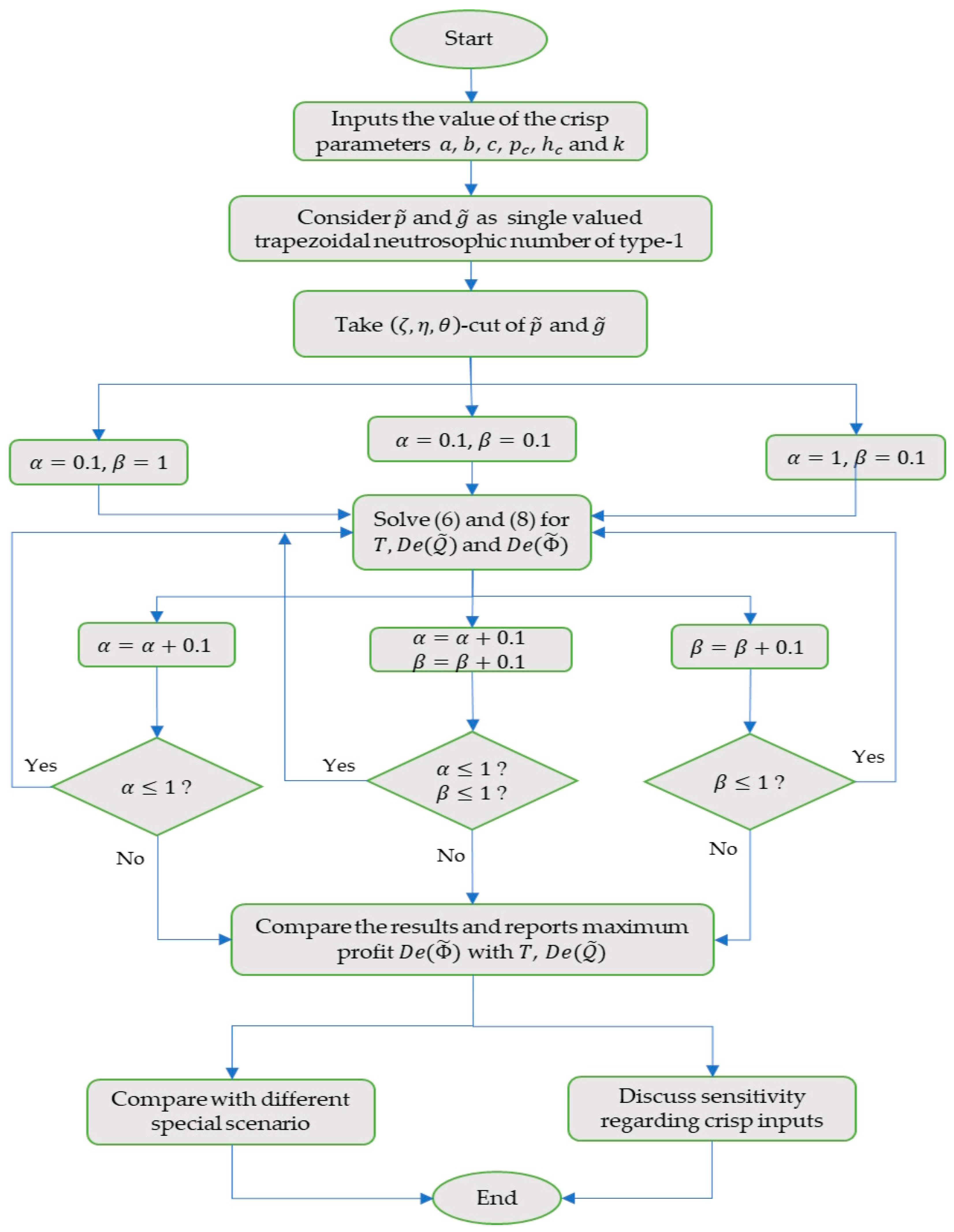
The optimal values of the decision variable and the objective functions for both cases are obtained using LINGO 20.0 software. The block diagram of solution methodology is depicted visually in Figure 3. Here, the effects of memory on the suggested inventory framework are explored by allowing the order of integration and differentiation to be expressed in fractional terms. The impacts of memory on the optimal values of the inventory cycle time $T$, order quantity $\mathcal{Q}$, and average profit $\mathsf{\Phi }$ concerning the integral and differential memory index and combined memory indexes are presented in

Table 4. Changes in optimal values of the inventory cycle time $\left(T\right)$, de-neutrosophied lot-size $De\left(\tilde{\mathcal{Q}}\right)$, and de-neutrosophied average profit $De\left(\tilde{\Phi }\right)$ concerning different values of differential memory index $\left(\alpha \right)$ for both the cases.

$\mathbf{Differential} \mathbf{Memory} \mathbf{Index} \left(\mathit{\alpha }\right)$	Case 1			Case 2
	$\mathit{T}$	$\mathit{D}\mathit{e}\left(\tilde{\mathcal{Q}}\right)$	$\mathit{D}\mathit{e}\left(\tilde{\mathit{\Phi }}\right)$	$\mathit{T}$	$\mathit{D}\mathit{e}\left(\tilde{\mathcal{Q}}\right)$	$\mathit{D}\mathit{e}\left(\tilde{\mathit{\Phi }}\right)$
0.1	399.8533	84.98810	1122.882	428.0261	92.22351	1124.149
0.2	79.80297	112.0913	1089.504	84.94239	122.3262	1092.688
0.3	31.90959	131.9303	1047.066	33.80194	144.6695	1052.386
0.4	17.27638	145.9316	1000.299	18.22578	160.6827	1007.685
0.5	11.10146	155.5457	952.9216	11.66983	171.8806	962.1324
0.6	7.958097	162.0517	907.4786	8.339468	179.6295	918.2022
0.7	6.149404	166.4758	865.5107	6.426379	185.0423	877.4214
0.8	5.015689	169.6026	827.8043	5.228787	188.9798	840.5969
0.9	4.259133	172.0114	794.6054	4.430374	192.0839	808.0119
1	3.729939	174.1285	765.8041	3.872264	194.8317	779.5998

,

Table 5. Changes in optimal values of the inventory cycle time $\left(T\right)$, de-neutrosophied lot-size $De\left(\tilde{\mathcal{Q}}\right)$, and de-neutrosophied average profit $De\left(\tilde{\Phi }\right)$ concerning different values of integral memory index $\left(\beta \right)$ for both of the cases.

$\mathbf{Integral} \mathbf{Memory} \mathbf{Index} \left(\mathit{\beta }\right)$	Case 1			Case 2
	$\mathit{T}$	$\mathit{D}\mathit{e}\left(\tilde{\mathcal{Q}}\right)$	$\mathit{D}\mathit{e}\left(\tilde{\mathit{\Phi }}\right)$	$\mathit{T}$	$\mathit{D}\mathit{e}\left(\tilde{\mathcal{Q}}\right)$	$\mathit{D}\mathit{e}\left(\tilde{\mathit{\Phi }}\right)$
0.1	0.1420908	7.177677	1133.716	0.1422021	7.290729	1133.381
0.2	0.5283476	27.47303	529.5268	0.5252357	28.11288	528.9679
0.3	1.104542	57.45527	525.6567	1.128991	63.29430	523.0880
0.4	1.066489	56.11404	547.8878	1.087412	61.66458	548.3217
0.5	1.106919	58.30946	551.7430	1.111686	63.11487	554.6196
0.6	1.498053	78.26965	565.3521	1.509363	84.99367	569.2447
0.7	1.946114	99.98734	596.0200	1.970221	109.0983	601.2870
0.8	2.466200	123.6140	640.0327	2.513656	135.7912	647.2208
0.9	3.064850	148.7674	696.5220	3.151041	164.8463	706.4436
1	3.729939	174.1285	765.8041	3.872264	194.8317	779.5998

, and

Table 6. Changes in optimal values of the inventory cycle time $\left(T\right)$, de-neutrosophied lot-size $De\left(\tilde{\mathcal{Q}}\right)$, and de-neutrosophied average profit $De\left(\tilde{\Phi }\right)$ concerning the combined effect of different values of the differential memory index $\left(\alpha \right)$ and integral memory index $\left(\beta \right)$ for both of the cases.

$\mathbf{Differential} \mathbf{Memory} \mathbf{Index} \left(\mathit{\alpha }\right)$	$\mathbf{Integral} \mathbf{Memory} \mathbf{Index} \left(\mathit{\beta }\right)$	Case 1			Case 2
		$\mathit{T}$	$\mathit{D}\mathit{e}\left(\tilde{\mathcal{Q}}\right)$	$\mathit{D}\mathit{e}\left(\tilde{\mathit{\Phi }}\right)$	$\mathit{T}$	$\mathit{D}\mathit{e}\left(\tilde{\mathcal{Q}}\right)$	$\mathit{D}\mathit{e}\left(\tilde{\mathit{\Phi }}\right)$
0.1	0.1	0.1417075	41.54867	1136.483	0.1418115	42.17316	1136.175
0.2	0.2	0.5816986	46.53076	544.2380	0.5802684	48.15235	543.8590
0.3	0.3	1.024004	52.38877	555.8626	1.032241	56.59897	555.2328
0.4	0.4	1.012930	52.88677	566.5520	1.022840	57.22225	567.2648
0.5	0.5	1.180058	57.22354	565.6360	1.180058	61.67388	567.6178
0.6	0.6	1.637833	70.24704	583.5185	1.641313	75.80669	586.2804
0.7	0.7	2.182657	88.72920	617.8234	2.197459	96.08327	621.8546
0.8	0.8	2.795628	114.0835	663.1403	2.839151	124.4849	669.2645
0.9	0.9	3.363199	144.6026	714.5164	3.456291	159.7256	723.8987
1	1	3.729939	174.1285	765.8041	3.872264	194.8317	779.5998

, respectively. One memory index is consistently maintained at a value of 1 during the evaluation of how other memory indexes affect the overall outcome.

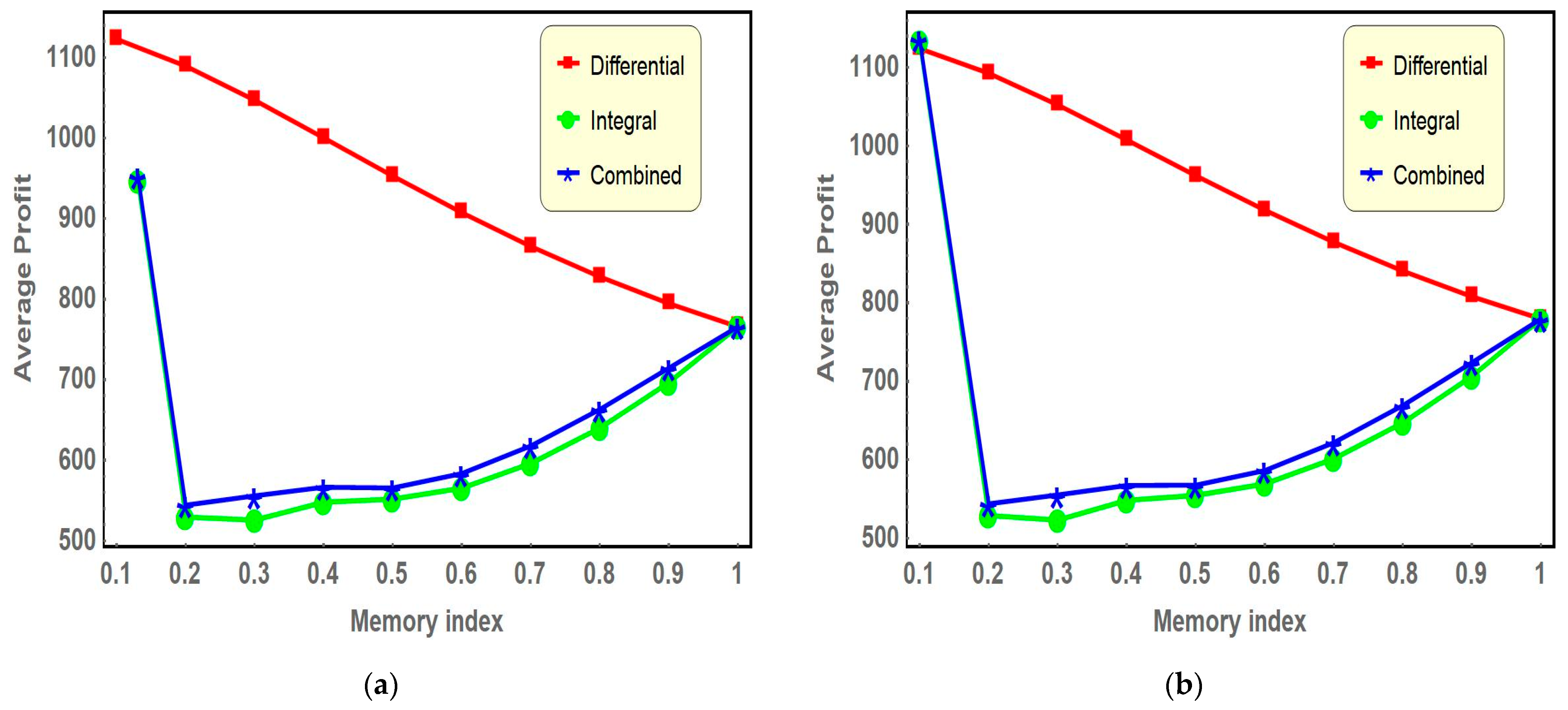
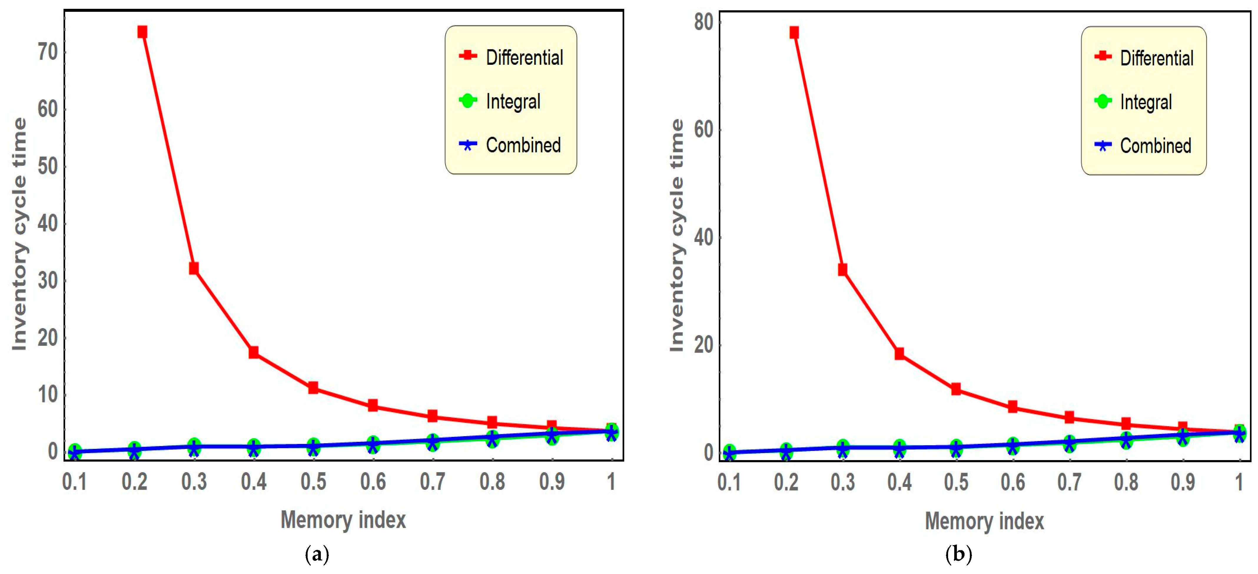
Figure 4, Figure 5 and Figure 6 visually illustrate the differences in the overall profit, the size of the lots, and the complete cycle time, respectively, showing how these elements change in relation to the memory indexes for both scenarios under consideration.

Based on the observations from Figure 4 for both scenarios, it is evident that as the differential memory indexes rise (that is, the memory effect in the inventory system decreases), the graphical representation of the average profit function consistently exhibits a downward trend. In contrast, when examining the situation involving the integral memory index and the scenario that incorporates combined effects, the average profit initially experiences a decline but subsequently rises, forming a distinctive L-shaped curve. The analysis reveals that under strong memory effects, incorporating both differential and integral memory indexes, the average profit can be enhanced by approximately 44–49% compared to scenarios without memory effects.

Figure 5 illustrates that a decrease in the differential memory index (implying a stronger memory effect within the inventory system) results in an extreme increase in the inventory cycle time. In contrast, a reduction in the integral memory index leads to a gradual decrease in the inventory cycle time. In the case of the combined memory effect, when both memory indexes decrease simultaneously, the inventory cycle time also shows a gradual declining trend, closely resembling the behavior observed under the influence of the integral memory index alone.

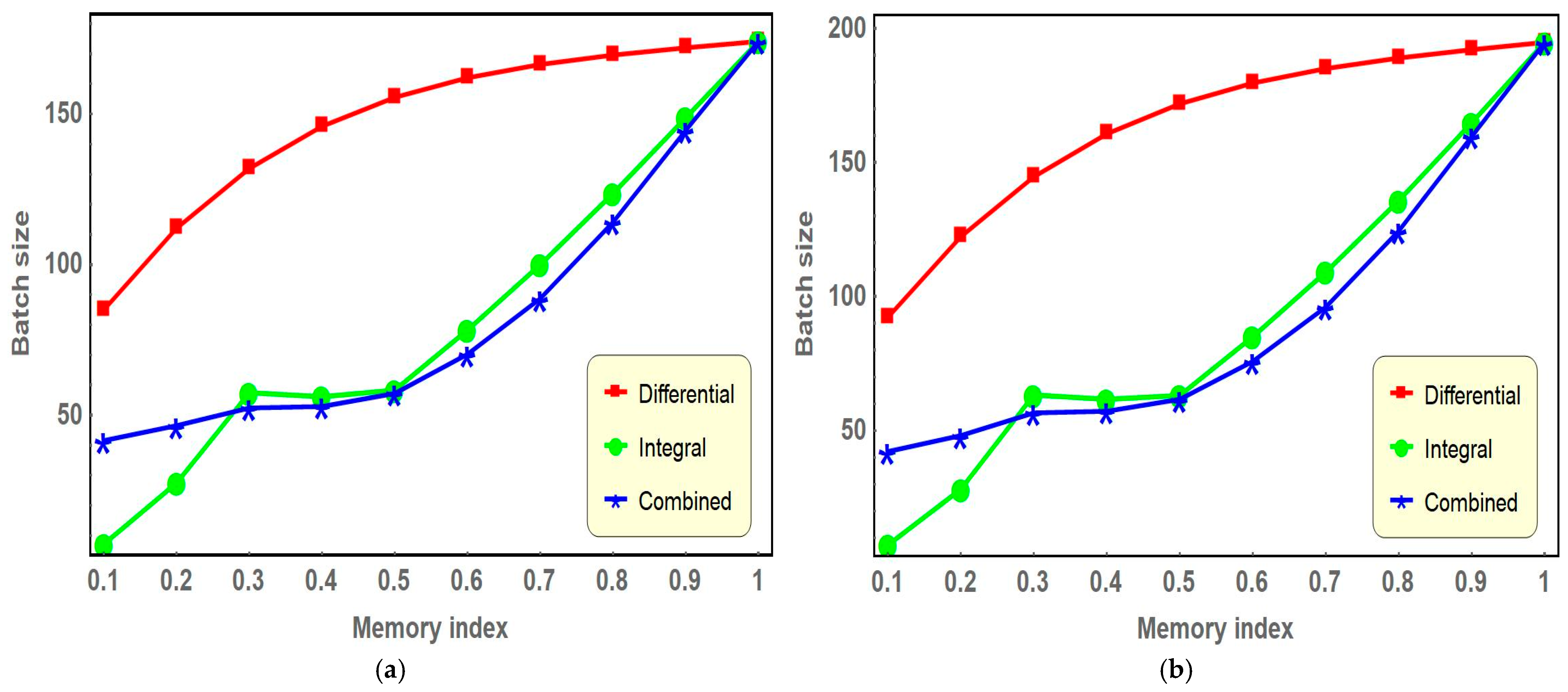
Based on the observations from Figure 6 in both scenarios, it can be noted that as the memory index rises, the graph depicting the optimal lot size values exhibits a modest upward trend initially, followed by a gentle decline. Nevertheless, the impact of the differential memory index on the lot size is significantly more pronounced when compared to the influence exerted by the integral memory index or the combined effect of both.

8.1. Comparison Among Different Special Scenario

Here, we have compared the optimal solutions of the proposed model with different special scenarios depending on the differential memory index $\alpha$, integral memory index $\beta$, and membership threshold $\zeta$, $\eta$, and $\theta$ related to parametric representation of the neutrosophic number. In the case of the fractional-order model, the parameters α and β are theoretically allowed to take any value between 0 and 1; however, the numerical analysis is carried out specifically for α = 0.1 and β = 0.1. The optimal values of decision variable and objective functions of Case I and Case II are presented in

Table 7. Optimal results for different special scenarios of Case I and Case II.

Scenarios	Conditions	Case I			Case II
		$\mathit{T}$	$\mathit{D}\mathit{e}\left(\tilde{\mathcal{Q}}\right)$	$\mathit{D}\mathit{e}\left(\tilde{\mathit{\Phi }}\right)$	$\mathit{T}$	$\mathit{D}\mathit{e}\left(\tilde{\mathcal{Q}}\right)$	$\mathit{D}\mathit{e}\left(\tilde{\mathit{\Phi }}\right)$
Integer order model in fuzzy environment	$\alpha =1$, $\beta =1$ $\zeta =\zeta$, $\eta =0$, $\theta =1-\zeta$ $0\le \zeta \le 1$	3.783146	181.1774	649.7950	3.823170	186.9887	653.6690
Integer order model in neutrosophic environment	$\alpha =1$, $\beta =1$ $0\le \zeta ,\eta ,\theta \le 1$	3.729939	174.1285	765.8041	3.872264	194.8317	779.5998
Fractional order model in fuzzy environment	$0<\alpha , \beta \le 1$ $\zeta =\zeta$, $\eta =0$, $\theta =1-\zeta$ $0\le \zeta \le 1$	0.1417074	41.58335	1105.004	0.1418116	42.10979	1104.727
Fractional order model in neutrosophic environment	$0<\alpha , \beta \le 1$ $0\le \zeta ,\eta ,\theta \le 1$	0.1417075	41.54867	1136.483	0.1418115	42.17316	1136.175

.

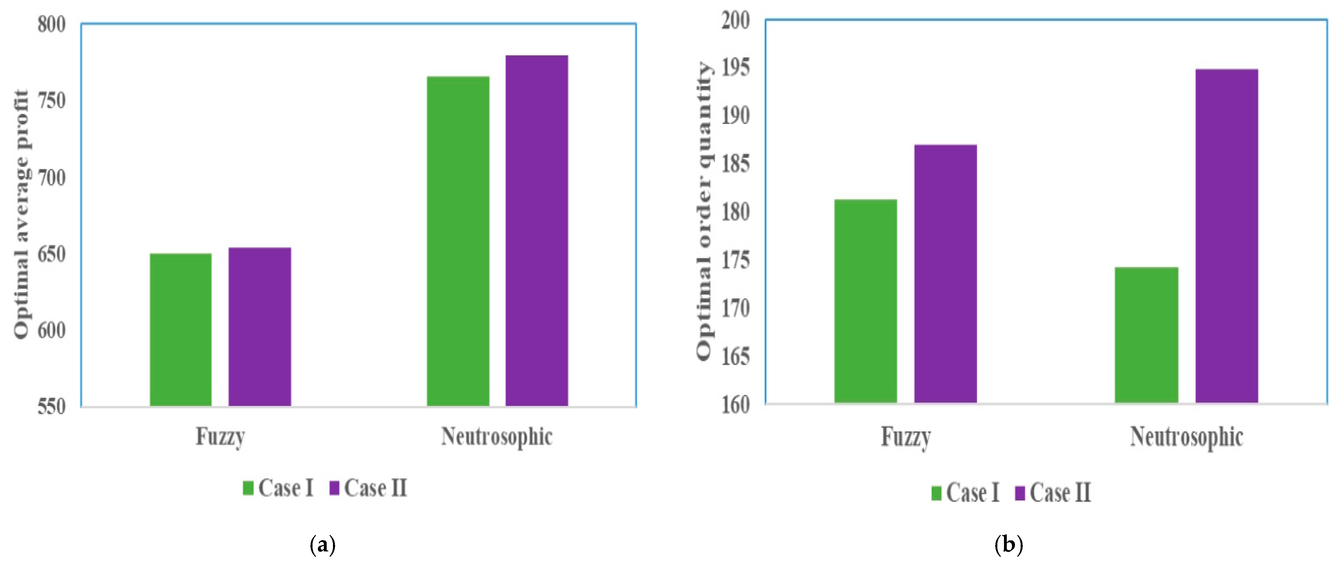
Table 7 clearly indicates that the fractional-order model within the neutrosophic environment generates the highest profit among all scenarios. Additionally, the average profit achieved under the neutrosophic setting surpasses those obtained in fuzzy environments. Moreover, the fractional-order model outperforms the integer-order model in terms of profit. For the integer-order model, a bar diagram of the optimal results under fuzzy and neutrosophic environments is illustrated in Figure 7. As shown in Figure 7a, the neutrosophic model yields a higher profit compared to the fuzzy model. Within the neutrosophic framework, Case II (associated with type-2 neutrosophic differentiability) outperforms Case I (based on type-1 neutrosophic differentiability) in terms of profitability. 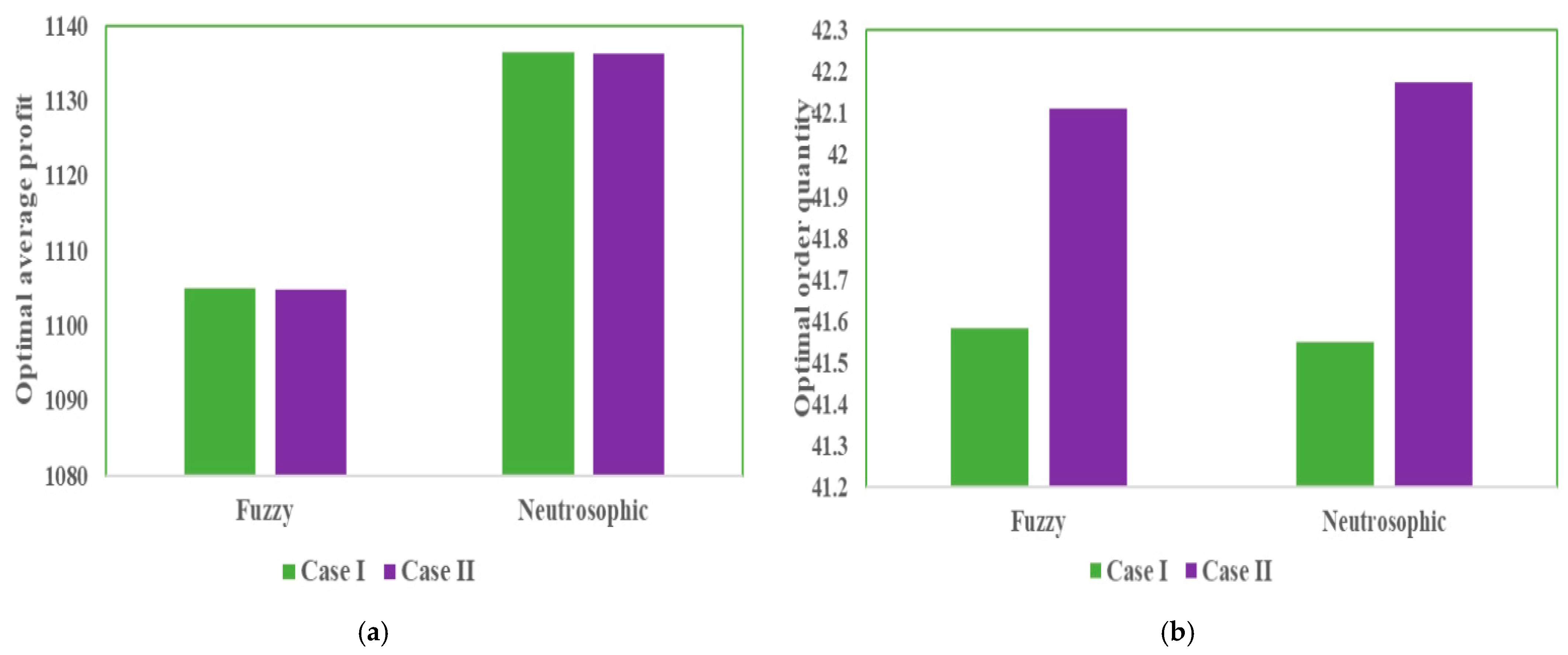Figure 7b further reveals that the optimal order quantity is lowest in Case I of the neutrosophic model compared to all other scenarios. For the fractional-order model, a bar diagram of the optimal results under fuzzy and neutrosophic environments is presented in Figure 8. From Figure 8a, it is clear that the neutrosophic model yields higher profit than the fuzzy model, similar to the integer order model. However, in the neutrosophic model, both the cases give approximately the same results. The optimal order quantity is lowest in the neutrosophic model of Case I than all other scenarios.

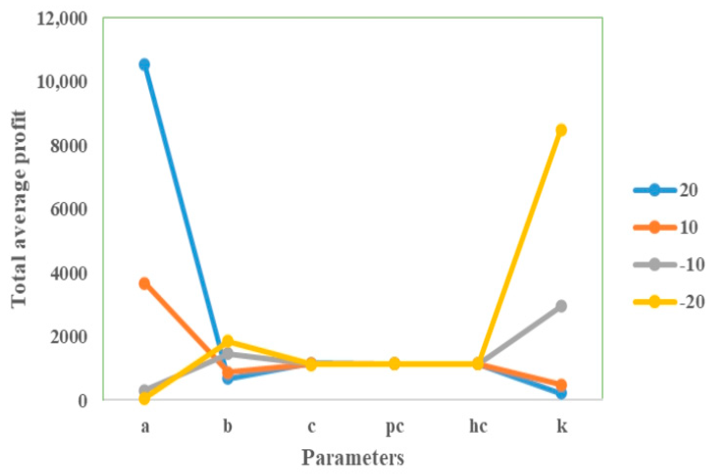
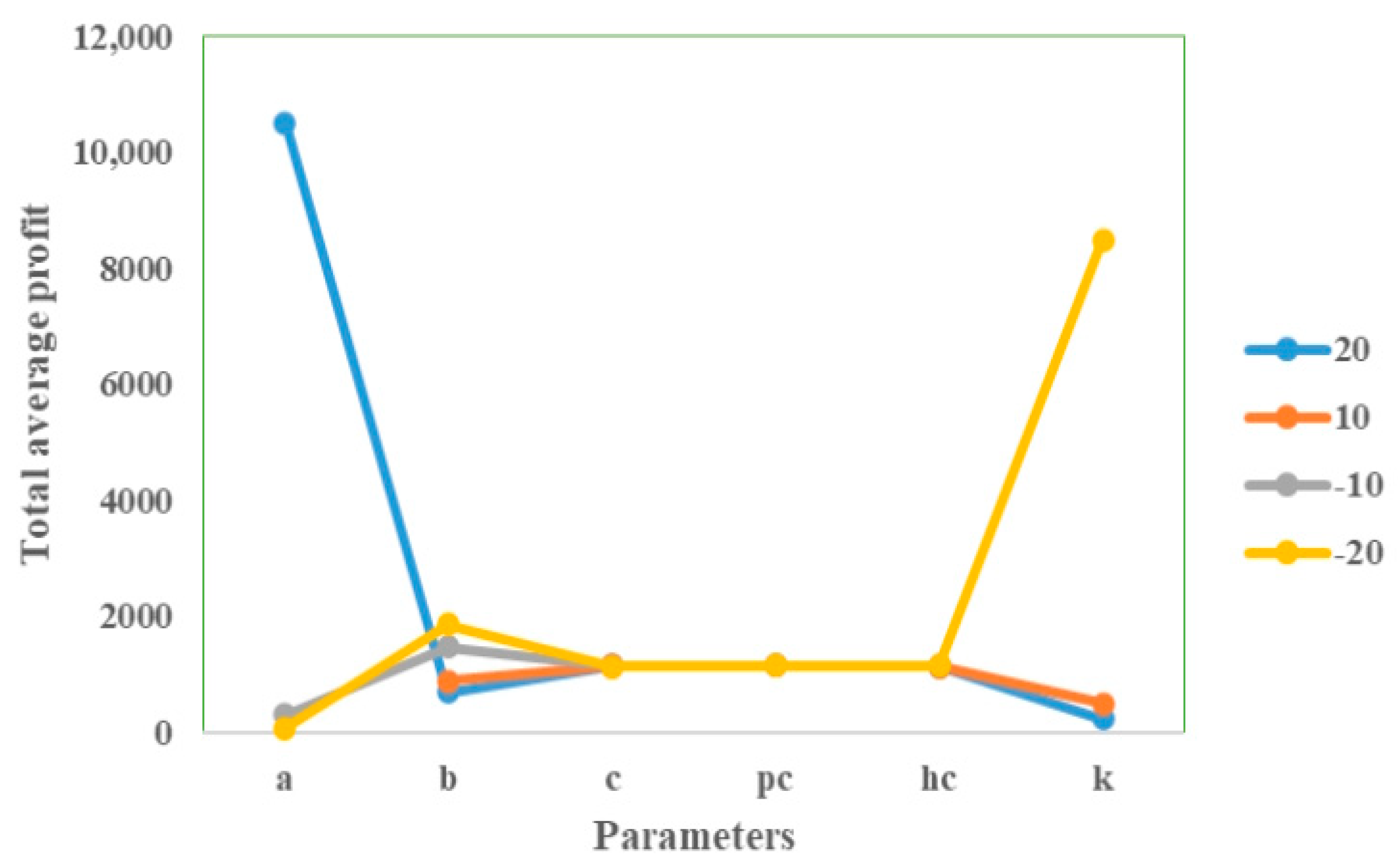
8.2. Sensitivity Analysis with Respect to Crisp Input Parameters

Based on the analysis presented in the preceding subsection, it can be concluded that the scenario involving the fractional-order model (with $\alpha =0.1$ and $\beta =0.1$) within the neutrosophic environment yields the best results for both the cases. So, in this subsection, an extensive sensitivity analysis is carried out for both considered cases to evaluate the influence of variations in the crisp input parameter on the optimal outcomes of the model. The chosen parameter is systematically varied within a range of −20% to +20%, while all other model parameters are maintained at their original values to isolate the effects of this single parameter change. The resulting sensitivity of the optimal solutions with respect to the crisp parameter is comprehensively presented in

Table 8. Sensitivity of optimal values with respect to crisp inputs.

Crisp Inputs	Change in %	Case I			Case II
		$\mathit{T}$	$\mathit{D}\mathit{e}\left(\tilde{\mathcal{Q}}\right)$	$\mathit{D}\mathit{e}\left(\tilde{\mathit{\Phi }}\right)$	$\mathit{T}$	$\mathit{D}\mathit{e}\left(\tilde{\mathcal{Q}}\right)$	$\mathit{D}\mathit{e}\left(\tilde{\mathit{\Phi }}\right)$
$a=60$	+20	0.014979	41.46861	10514.02	0.014986	41.97917	10512.25
	+10	0.043259	41.50393	3677.114	-	2.198760	0.9973367 × 1016
	−10	0.544751	41.60717	300.3120	0.5452745	42.31089	300.2034
	−20	2.583933	41.68727	64.63202	2.587283	42.49438	64.59962
$b=0.6$	+20	0.2440575	41.64445	678.9534	0.2442971	42.41253	678.6983
	+10	0.1852840	41.59497	881.4167	0.1854419	42.29005	881.1344
	−10	0.1091412	41.50536	1455.912	0.1092097	42.06141	1455.581
	−20	0.0846196	41.46484	1853.693	0.08466457	41.95435	1853.343
$c=0.4$	+20	0.1399580	41.54831	1150.689	0.1400611	42.17316	1150.377
	+10	0.1408298	41.54849	1143.566	0.1409335	42.17317	1143.255
	−10	0.1425912	41.54885	1129.439	0.1426960	42.17317	1129.132
	−20	0.1434813	41.54904	1122.434	0.1435867	42.17318	1122.129
$p_c=5$	+20	0.1417070	41.54866	1136.485	0.1418113	42.17316	1136.177
	+10	0.1417072	41.54867	1136.484	0.1418115	42.17316	1136.176
	−10	0.1417076	41.54868	1136.481	0.1418117	42.17317	1136.173
	−20	0.1417080	41.54869	1136.479	0.1418120	42.17318	1136.171
$h_c=2$	+20	0.1421207	41.56077	1133.482	0.1422462	42.18607	1133.113
	+10	0.1419139	41.55472	1134.981	0.1420286	42.17962	1134.643
	−10	0.1415014	41.54263	1137.985	0.1415949	42.16671	1137.707
	−20	0.1412957	41.53659	1139.488	0.1413787	42.16027	1139.242
$k=700$	+20	0.8800258	49.87321	219.6649	0.8808001	50.62357	219.5935
	+10	0.3680951	45.71028	481.3348	0.3683924	46.39766	481.1913
	−10	0.04933808	37.38834	2937.360	-	1.964495	0.8912118 × 1016
	−20	0.01517133	33.22923	8489.942	0.01518030	33.72819	8488.093

. Furthermore, to enhance clarity and facilitate better understanding, a visual representation of the tabulated results is provided through Figure 9 and Figure 10. The key observations and insights derived from this analysis are summarized as follows:

The key observations and insights derived from this analysis are summarized as follows:

• The fixed component $\left(a\right)$ of the demand rate is highly positively sensitive to profitability, meaning that even small increases in baseline demand can significantly enhance profits.
• The selling price potential $\left(b\right)$ is negatively associated with average profit, as increasing the selling price tends to reduce demand. This underscores the importance of carefully balancing pricing strategies. The higher prices may improve per-unit margins, but they can lead to a decline in sales volume that outweighs the margin gains, ultimately reducing overall profitability.
• Another important observation is that increasing the green level potential $\left(c\right)$ of the item positively influences profitability, as demand tends to rise for green products. Managers should consider enhancing the sustainability attributes of their inventory, as promoting greener products can drive higher sales and improve overall profit margins.
• The unit holding cost $\left(h_c\right)$ and purchasing cost $\left(p_c\right)$ exhibit limited sensitivity to the overall profit function, while the ordering cost $\left(k\right)$ plays a much more critical role. This suggests that small variations in ordering cost can significantly impact profitability. Therefore, targeted interventions aimed at controlling and reducing ordering costs can serve as a more effective lever for enhancing overall inventory profitability.

8.3. Discussions and Managerial Insights

We analyze both scenarios of NCFD for the on-hand inventory level based on two types of generalized neutrosophic differentiability. Upon reviewing the tables and figures, we can outline the following observations:

• The profit can be optimized by incorporating the stronger memory sense in the proposed EOQ model. The small value of the memory index implies the strong memory while unity regarding the memory index implies memory-free phenomena. From Table 6 and Figure 4, it is noted that the average profit in a memory-free environment is USD 765.8041 for a cycle time of 3.729939 years and order size of 174.1285 units in the first case of neutrosophic differentiability. In the alternative case, the optimal value of the objective function and decision variables are USD 779.5998, 3.872264 years, and 194.8317 units, respectively. Incorporation of soft or local memory exhibits inferior results compared to the memory-free environment. However, optimal results are given at a memory index of 0.1 with a strong memory sense where the optimal value of the objective function and decision variables are USD 1136.483, 0.147075 years, and 41.54867 units in the first case of neutrosophic differentiability and USD 1136.175, 0.1418115 years, and 42.17316 units in the second case of neutrosophic differentiability. Therefore, the managerial implication concerning profit is as follows:

  $$Strong memory>No memory>Weak memory$$
• The demand pattern was assumed to be imprecise due to its vague association with retail price and green level. Therefore, impacts of uncertain price and greenness are put into the model as conflicting or contradictory information, a common scenario in real-world socio-economic phenomena. We consider triangular neutrosophic numbers to present the incompleteness, inconsistency, and indeterminacy. Furthermore, there is a dedicated section, namely Section 8.1, for comparing the numerical simulation of the same models in crisp and fuzzy environments with and without memory. Table 7 shows that the highly expressive sense of uncertainty guaranteed by the neutrosophic environment provides the best results in terms of profit. The pattern regarding average profit, irrespective of the memory presence, is as follows:

  $$\mathrm{N}\mathrm{e}\mathrm{u}\mathrm{t}\mathrm{r}\mathrm{o}\mathrm{s}\mathrm{o}\mathrm{p}\mathrm{h}\mathrm{i}\mathrm{c} \mathrm{e}\mathrm{n}\mathrm{v}\mathrm{i}\mathrm{r}\mathrm{o}\mathrm{n}\mathrm{m}\mathrm{e}\mathrm{n}\mathrm{t}>\mathrm{F}\mathrm{u}\mathrm{z}\mathrm{z}\mathrm{y} \mathrm{e}\mathrm{n}\mathrm{v}\mathrm{i}\mathrm{r}\mathrm{o}\mathrm{n}\mathrm{m}\mathrm{e}\mathrm{n}\mathrm{t}>\mathrm{C}\mathrm{r}\mathrm{i}\mathrm{s}\mathrm{p} \mathrm{e}\mathrm{n}\mathrm{v}\mathrm{i}\mathrm{r}\mathrm{o}\mathrm{n}\mathrm{m}\mathrm{e}\mathrm{n}\mathrm{t}$$
• Employment of memory and expert opinions under uncertainty, in a paradoxical sense, provides the best result. However, the manager has to reduce the length of the decision cycle and the lot size to reach the profit goal.

8.4. More Possible Applications of the Proposed Theory

In this subsection, we hint at some more applications of the FC for neutrosophic-valued functions.

8.4.1. Financial Modeling

Financial models include factors such as historical data regarding pricing, behavior of the consumers and investors, etc. The forecasting and optimization in decision making based on the past activities can be renamed as memory influenced. On the other hand, uncertainty and contradiction may come into the decision process as an integral part due to socio-political and psychological reasons. In this context, the proposed theory of FC for neutrosophic-valued functions can be used to analyze risks under conflicting opinions by various experts, to forecast the market pattern and optimal pricing.

8.4.2. Reliability Theory

The theory of reliability is about measuring system failure probabilities, component life expectancy, etc. Now, the degradation in efficiency may be memory influenced. Moreover, there may be incomplete failure data or conflicting maintenance records in the hand of the strategist. In such a case, the FC for neutrosophic-valued functions can fulfill the purposes regarding safety estimation and decision support.

9. Conclusions

In this paper, we have introduced FC for neutrosophic-valued functions and hinted at several applications. In particular, an EOQ model has been designed and analyzed in light of the proposed theory. Co-existence of the memory and paradoxical opinion-based information necessitates the theory of fractional calculus for neutrosophic-valued functions.

In this study, we defined fractional order integration in the Riemann–Louville sense and fractional order derivatives in both the Riemann–Louville and Caputo senses within the neutrosophic framework. While the primary focus is on advancing the theoretical foundations of FC in uncertain contexts, the paper also illustrates a practical application through a lot-sizing model incorporating demand influenced by the price and greenness of the items. Lower memory index values indicate enhanced memory capabilities. Numerical simulations of the lot-sizing model indicate that incorporating strong memory effects, represented by a low memory index (0.1), can enhance average profit by approximately 44% to 49% compared to memory-independent scenarios (with memory index 1). Furthermore, decision-making under a neutrosophic environment demonstrates superior profitability when compared to both precise (crisp) and imprecise (fuzzy or intuitionistic fuzzy) modeling frameworks, highlighting its effectiveness in handling indeterminacy and conflicting information.

Despite the novel introduction of FC for neutrosophic-valued functions and fitted domain of application, the present study has some shortcomings that can be minimized in the following ways in future:

• An EOQ model for single item–single vendor has been discussed as an immediate application of the proposed theory. However, the real-world financial market is far more complicated than the adapted model. Considering coordination and competition among multiple players in supply chain scenarios in the proposed direction can fulfill the ultimate purpose in this regard. Furthermore, real-world data from industries can verify the applicability of the proposed model in a crystal manner.
• To use the proposed theory in more realistic inventory or supply chain management phenomena, more developments on fractional differential equations for neutrosophic-valued functions are needed. More precisely, the theory of the existence and uniqueness conditions for the solvability of such a fractional differential is urgently needed.