Heterogeneity of Deep Tight Sandstone Reservoirs Using Fractal and Multifractal Analysis Based on Well Logs and Its Correlation with Gas Production

Abstract

Deep tight sandstone reservoirs are characterized by low porosity and permeability, complex pore structure, and strong heterogeneity. Conducting research on the heterogeneity characteristics of reservoirs could lay a foundation for evaluating their effectiveness and accurately identifying advantageous reservoirs, which is of great significance for searching for “sweet spot” oil and gas reservoirs in tight reservoirs. In this study, the deep tight sandstone reservoir in the Dibei area, northern Kuqa depression, Tarim Basin, China, is taken as the research object. Firstly, statistical methods are used to calculate the coefficient of variation (CV) and coefficient of heterogeneity (TK) of core permeability, and the heterogeneity within the reservoir is evaluated by analyzing the variations in the reservoir permeability. Then, based on fractal theory, the fractal and multifractal parameters of the GR and acoustic logs are calculated using the box dimension, correlation dimension, and the wavelet leader methods. The results show that the heterogeneity revealed by the box dimension, correlation dimension, and multifractal singular spectrum calculated based on well logs is consistent and in good agreement with the parameters calculated based on core permeability. The heterogeneity of gas layers is comparatively weaker, while that of dry layers is stronger. In addition, the fractal parameters of GR and the acoustic logs of three wells with the oil test in the study area were analyzed, and the relationship between reservoir heterogeneity and production was determined: As reservoir heterogeneity decreases, production increases. Therefore, reservoir heterogeneity can be used as an indicator of production; specifically, reservoirs with weak heterogeneity have high production.

1. Introduction

In recent years, an increasing number of researchers have begun to focus on deep and ultra-deep oil and gas resources [1,2,3]. In China’s oil exploration, formations in the eastern plains and coastal areas with depths between 3500 and 4500 m are classified as “deep formations”, while those exceeding 4500 m are referred to as “ultra-deep formations”. In western China, formations with depths between 4500 and 6000 m are defined as “deep formations”, and those exceeding 6000 m are called “ultra-deep formations” [4,5]. Ultra-deep oil and gas exploration in China is primarily concentrated in the Tarim, Junggar, and Sichuan Basins. In the Kuqa Sag of the Tarim Basin, well Bozi-9 has achieved high production rates of 41.82 × 10⁴ m³ of gas per day and 115.15 m³ of oil per day at a depth of 7700 m in the Cretaceous Bashkirchik Formation sandstone. The Triassic Karamay Formation of well Zheng-10 in the central Junggar Basin has been tested for 7530 m³ of gas per day and 78.18 m³ of oil per day at a depth of 6800 m. In those regions, deep and ultra-deep resources show great potential and play crucial roles in supplementing conventional oil and gas reserves [6,7].

Deep tight sandstone reservoirs typically exhibit complex pore structures, poor connectivity, and strong heterogeneity [8]. These reservoirs have undergone complex sedimentation, diagenesis, and post-depositional tectonic modifications during long-term geological evolution, resulting in heterogeneous spatial distributions and internal property variations [9]. The ambiguous characterization of heterogeneity in deep tight sandstone reservoirs hinders successful natural gas exploration and development.

Studies on reservoir heterogeneity originate from geological core analysis, where parameters such as variation coefficients and range values are used to assess heterogeneity of permeability. Other studies have employed statistical methods such as variance analysis, standard deviation calculations, Lorenz coefficients, and Dikstra–Persson coefficients (VDP) for core data or well logs to quantify heterogeneity [10,11]. Lake and Jensen (1991) compared dynamic and static calculation methods to analyze the differences between Lorenz coefficients and VDP coefficients, describing their correlation with heterogeneity [12]. Fitch et al. (2013) evaluated the Lorenz coefficient as a metric for quantifying the heterogeneity of core data [13]. They analyzed how population variability impacts heterogeneity measurements and applied this approach to wireline-derived porosity and permeability data to compare reservoir unit heterogeneity. Hosseinzadeh and Tavakoli (2024) employed the Lorenz coefficient to calculate heterogeneity and documented primary sedimentary and secondary diagenetic alterations through thin section analysis [14]. Farooq et al. (2019) investigated the definition and quantification of the term heterogeneity through a suite of statistical measures, including Lorenz and VDP coefficients in Tal Formation carbonate rocks [15]. These metrics enable the interpretation of variations in well log data, allowing for a comparison of heterogeneity within single and multi-layered reservoir units. Tavoosi et al. (2021) employed multiple parameters, including CV, VDP, and the Lorenz coefficient, for a quantitative assessment of different scales of heterogeneity of carbonate sequences [16]. Davies et al. (2023) proposed a new methodology for quantifying heterogeneity on any continuous data and quantitatively analyzed the relationships between heterogeneity and the properties of carbonate formations in the North Sea [17]. The methods mentioned above have been successfully used in different study areas.

Furthermore, fractal dimensions have emerged as critical features for characterizing heterogeneity. Mostly, fractal geometry analysis based on core data in a laboratory is a promising method to interpret the pore structures in geoscience. The pore space of rocks has been investigated based on its fractal geometry, a method proposed by Mandelbrot [18]. According to fractal theory, the pore volumes of rocks have self-similar features [19]. The fractal dimension (D) is a vital parameter to characterize the regularity of self-similar structures and to indicate the complexity and heterogeneity of pore geometry [20,21,22]. Billi and Storti (2004) reported on the fractal dimensions of grain size distribution in carbonate clastic rocks that originated from the core of the regional strike–slip fault zone in the foreland of the Southern Apennine Mountains in Italy, reporting values ranging from 2.09 to 2.93 [23]. Based on SEM images, Xie et al. (2010) studied the fractal characteristics of Jurassic marine carbonate reservoir samples in the western Hubei and eastern Sichuan regions of China, determining the fractal dimensions of high gas-bearing reservoirs [24]. Xia et al. (2025) revealed the influence of pore–throat fractal characteristics on macroscopic reservoir permeability by analyzing MICP-derived capillary pressure curves [25]. Liu et al. (2004) used homogenization theory to establish a two-dimensional numerical model of rock and introduced the Weibull statistical method to simplify the modeling of heterogeneity [26]. Liu et al. (2016) made advances to a fractal capillary pressure model by introducing a “matchstick-like” tubular pore model specifically for evaluating the coal rock structures [27]. Zhou et al. (2023) systematically demonstrated the correlation between experimental fractal features and reservoir quality and established a fractal parameter-based methodology for reservoir quality prediction [28]. Liu et al. (2023) and Peng et al. (2020) achieved quantitative evaluations of reservoir heterogeneity intensity through fractal dimension extraction and inflection point analyses of the pore distribution in capillary pressure curves [29,30].

Studies have also indicated that calculating the fractal dimension of well logs provides an effective method for determining reservoir heterogeneity. In a single fractal analysis of well logs, box counting and correlation dimensions are the most commonly used. Liu et al. applied these methods to acoustic logs for fracture identification [31], and Wen integrated multiple fractal computation approaches (including acoustic log analysis) and established correlations between fractal dimensions and heterogeneity through the inversion of logs [32]. Mou studied the fractal characteristics of well logs in the Liaohe oil field using the box counting method, revealed the corresponding relationship between volcanic rock lithology and fractal dimension, and verified the feasibility of predicting volcanic rock lithology based on the fractal dimension of well logs [33].

Multifractal theory enhances heterogeneity characterization by introducing concepts such as generalized fractal dimensions and singularity spectra, which quantify both local and global structural variations. The box counting method is commonly used to calculate the multifractal parameters based on physical and log curves. Zhao et al. (2017) and Yan et al. (2017) investigated pore structures through a multifractal analysis of NMR data and by controlling factors of heterogeneity in pore structures [34,35]. Zhao et al. (2019) analyzed NMR and low-temperature N₂ adsorption experimental data and calculated the multifractal dimensions to evaluate the heterogeneity of pore structure [36]. Lv et al. (2025) also used the box dimension method to analyze the array sound wave pattern and achieved fracture identification [37]. However, the box counting method is not typically suitable for analyzing one-dimensional log curves, while wavelet-based fractal approaches, including wavelet and detrended fluctuation analysis (DFA), are employed more often for computing multifractal characteristics of one-dimensional log curves.

Lozada-Zumaeta et al. (2012) used the R/S (rescaled range) fractal model and interpolation method to estimate the spatial distribution of rock physics properties, such as effective porosity, permeability, and shale volume [38]. Partovi and Sadeghnejad (2017) proposed an automatic well-to-well comparison method based on fractal parameters [39]. Wavelet transform has been used to analyze the gamma, density, and acoustic logs, and automatic boundary detection has been achieved on an Iranian oil field. López et al. (2007) implemented a wavelet-driven fractal analysis combined with waveform classifiers to determine the fractal parameters across diverse log types [40]. Subhakar et al. (2016) conducted comparative fractal/multifractal studies using detrended fluctuation analysis (DFA) and wavelet transforms, employing multifractal logging features to identify geological boundaries while benchmarking the results against those of wavelet methods [41]. Amoura et al. (2022) applied the wavelet-derived fractal dimensions to velocity logs, interpreting lithology and heterogeneity through multifractal spectrum morphology and positional characteristics [42]. Rahul Prajapati (2024) used the Hurst index based on the wavelet leader method in the multifractal to quantify the variation in rock properties in shale exploration intervals [43]. Those studies indicate that the wavelet leader method could be used to characterize heterogeneity.

In the above studies, many scholars have used fractal parameters to characterize the heterogeneity of reservoirs, but the application of heterogeneity in oil and gas exploration and development is relatively rare. In this study, to comprehensively evaluate the heterogeneity of deep tight sandstone reservoirs, different methods, including statistical methods based on core permeability and fractal and multifractal analyses on well logs, were used. This study begins with a concise overview of the gas-bearing formations in the target Dibei region in the Tarim Basin, China, and then provides a detailed exposition of two methods: (1) heterogeneity characterization through a core analysis and (2) computational methodologies employing fractal dimension quantification. The calculated fractal dimensions based on well logs are integrated with core analytical data to systematically analyze reservoir heterogeneity in the target region. Furthermore, the qualitative correlation between fractal parameters and production was newly analyzed and found.

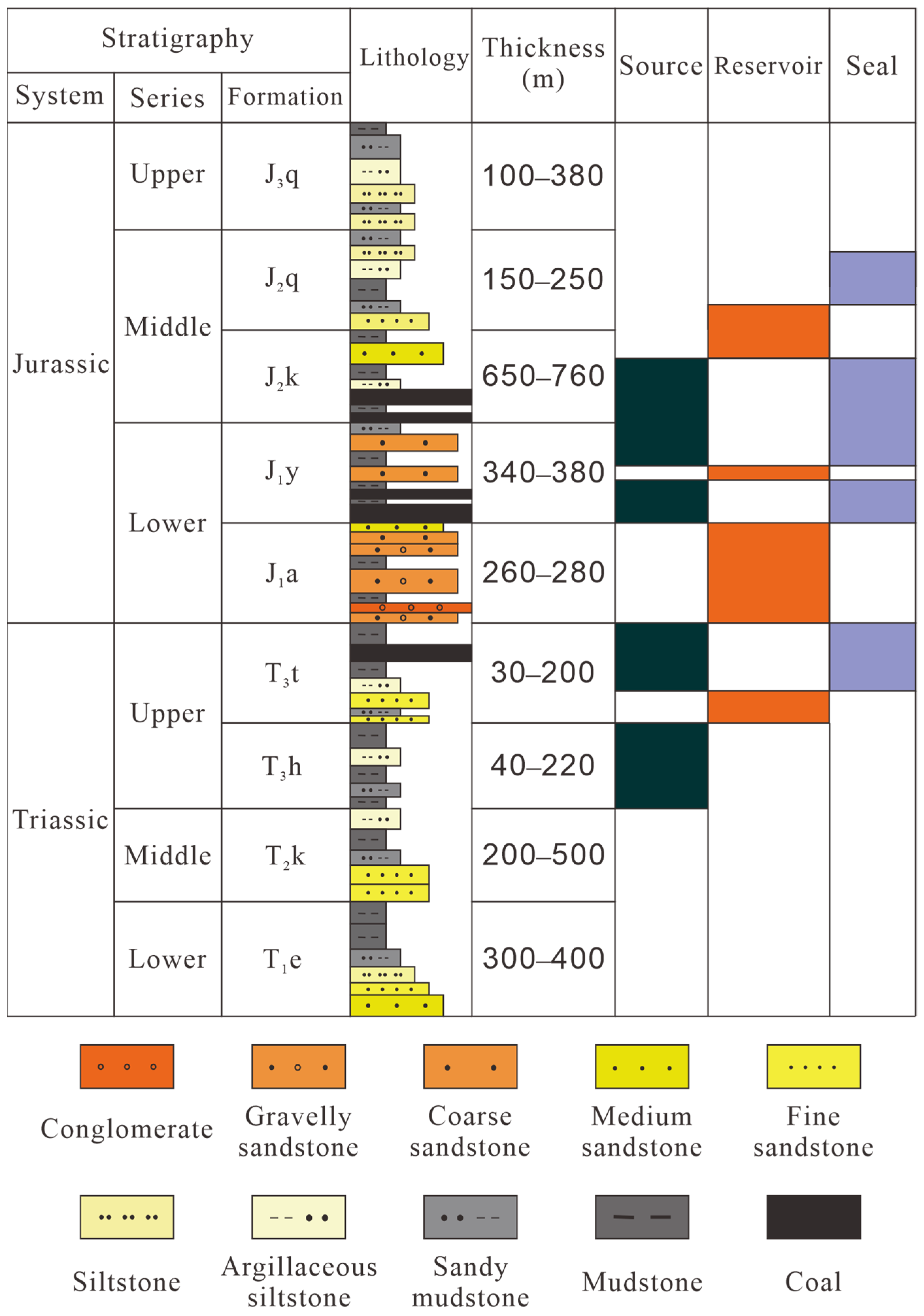
2. Geological Setting

This study took place in the Kuqa Formation located at the northern margin of the Tarim Basin, West China. The Kuqa Depression, a foreland basin developed on the Paleozoic folded basement, exhibits an overall north-high–south-low topography influenced by southward thrusting of the South Tianshan orogenic belt. The Kuqa area forms a transitional region between the South Tianshan structural zone and the Tarim Plate (Figure 1). The gas layers primarily studied here are the Jurassic Ahe Formation tight gas layers, with almost all formations extending to depths exceeding 4500 m. The overlying Jurassic Yangxia Formation consists of dark mudstone and a small amount of coal-bearing strata, which can be stably distributed and can form a good cap rock. The underlying Triassic Taliqike Formation also included dark mudstone and exists as the bottom plate of the gas reservoir.

The Yiqikelike structural belt of the Kuqa Depression exhibits favorable petroleum geological conditions. The Dibei gas reservoir demonstrates extensive contiguous distribution, where strong reservoir heterogeneity facilitates hydrocarbon accumulation in localized reservoirs independent of structural traps. Both the underlying Tariqike Formation and overlying Yangxia Formation contain thick, widespread coal seams with high organic matter abundance, serving dual roles as source rocks and effective seals. The tight sandstone reservoirs have undergone prolonged diagenetic evolution and tectonic modifications, exhibiting intricate pore structures and pronounced heterogeneity due to polygenetic controls (sedimentary, diagenetic, and tectonic) [44]. Stratigraphically, it comprises three units from top to bottom: sandy conglomerates interbedded with mudstone (J₁a¹), upper sandy conglomerates (J₁a²), and lower sandy conglomerates (J₁a³). Depositionally, the Ahe Formation represents braided river delta plain subfacies with low compositional maturity, dominated by (pebbly) coarse-to-medium sandstones. The thickness of the sand ranges from 250 m to 300 m. Vertically, it manifests as the superposition of multiple river channel sediments, with the thickness of a single river channel being about 1–2 m, while the cumulative thickness of multiple river channels can reach about 20 m. Laterally, frequent channel migrations result in continuous planar distribution [45,46].

Spatially, the source rocks and the Jurassic Ahe reservoirs form a “sandwich-style” interlayer (Figure 2), constituting an optimal source–reservoir–cap rock assemblage. This tightly arranged oil and gas injection system improves the efficiency of oil and gas drainage, which is beneficial for oil and gas trapping in tight sandstone reservoirs. This is a key factor in the formation of natural gas reservoirs in the northern part of Kuqa [47,48].

Figure 1. Structural position of the Dibei gas reservoir (modified from Li et al., 2024 [49]).

Figure 1. Structural position of the Dibei gas reservoir (modified from Li et al., 2024 [49]).

Figure 2. Stratigraphic column of hydrocarbon storage and cover combination in the northern Kuqa structural belt (modified from Li et al., 2024 [49]).

Figure 2. Stratigraphic column of hydrocarbon storage and cover combination in the northern Kuqa structural belt (modified from Li et al., 2024 [49]).

The distribution of core porosity and permeability is shown in Figure 3. Porosity ranges from 4% to 8%, with an average value of 5.94%. The permeability is mainly distributed from 0.1 mD to 5 mD, with an average of 0.82 mD, constituting a tight reservoir.

Four wells were used in this study, as their wellbore conditions were relatively good and the quality of logging data was high. In addition, two of the wells have rich core data. The information on the four well logs is shown in

Table 1. The base data for four wells.

Wells	YN4	YN2C	DB101	DB102
Depth intervals (m)	285	32	297	284
Average core permeability (mD)	0.704	0.44	/	0.04
Oil test (m3/day)	/	67,320 (gas)	5851 (gas)	16,328 (gas)

.

3. Calculation of Heterogeneity

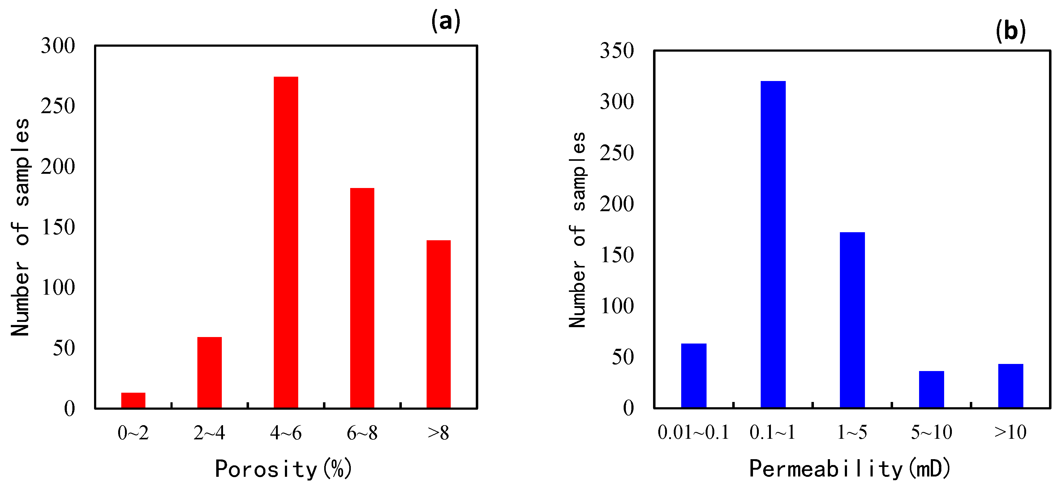
3.1. Heterogeneity Based on Core Permeability

The intralayer heterogeneity of reservoir layers is affected by particle size and the mud interlayer, which further affects the physical properties of the reservoir. Core permeability characterizes heterogeneity by calculating the coefficient of heterogeneity (TK) and coefficient of variation (CV), which collectively delineate the development characteristics of reservoir heterogeneity [50]. The coefficient of variation is defined as the ratio of standard deviation (SD) to mean permeability (MN), while the coefficient of heterogeneity represents the ratio of maximum permeability (MAX) to mean permeability (MN). The mathematical expressions are as follows:

$$CV=\left({\displaystyle \frac{SD}{MN}}\right)$$

(1)

$$TK=\left({\displaystyle \frac{MAX}{MN}}\right)$$

(2)

where CV is the coefficient of variation, SD is the standard deviation, MN is the average value, TK is the coefficient of heterogeneity, and MAX is the maximum value of the core permeability.

The calculation results were further compared with fractal dimension calculations.

3.2. Methods for Calculating Fractal Dimensions

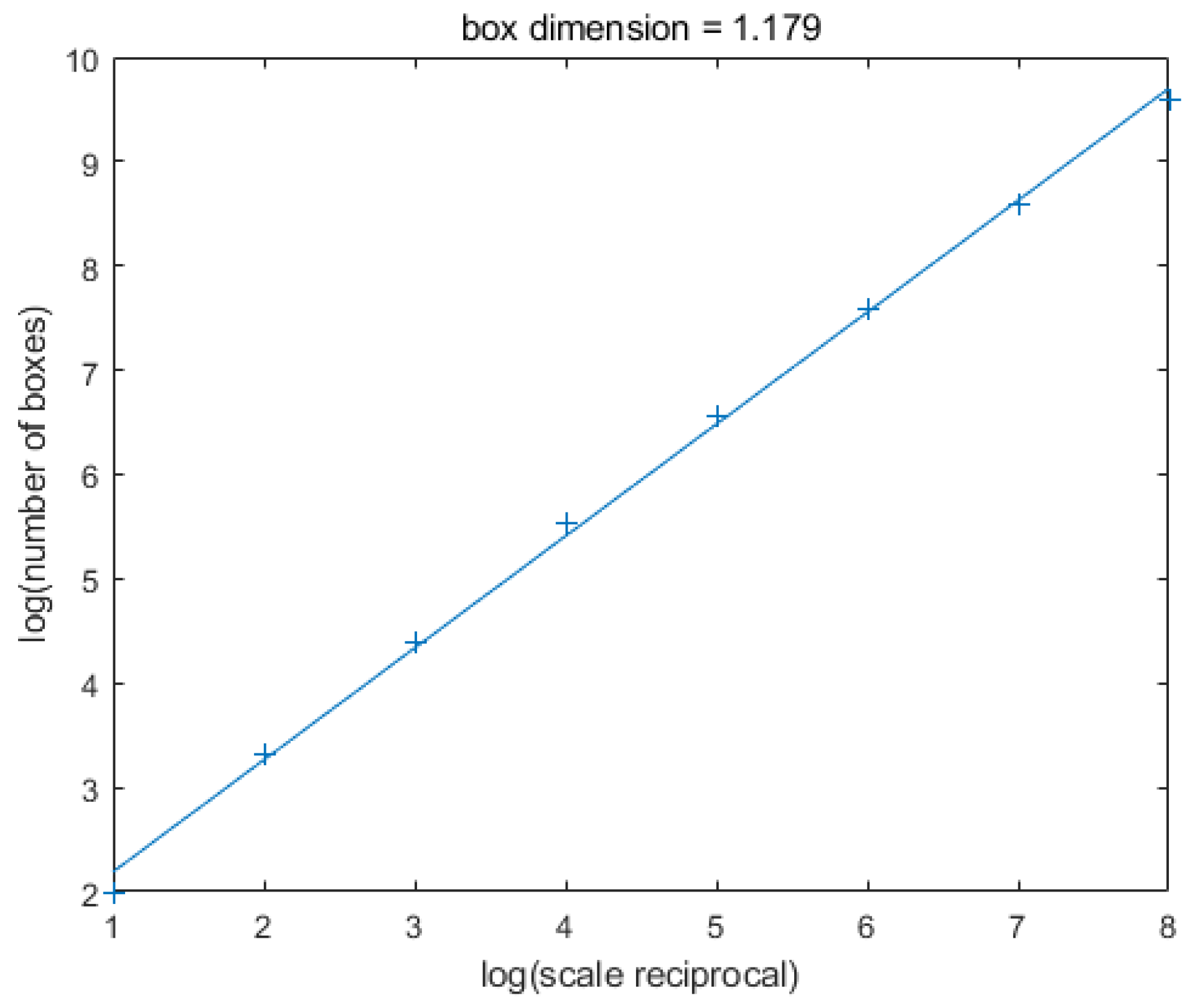
3.2.1. Box Dimension Method

Mandelbrot established fractal theory and applied nonlinear concepts such as self-similarity and fractal dimension to characterize these complex phenomena [18]. The fractal dimension method effectively quantifies the complexity and self-similarity of signals. When applied to well log curves, the magnitude of the fractal dimension can indicate the intensity of heterogeneity. In practical calculations, the fractal dimension is typically defined as the limit value when the measurement scale δ approaches zero. To formalize this, suppose a planar curve F is enclosed within a bounded interval. By progressively reducing the unit measurement length δ and recording the corresponding coverage count M_δ(F), the dimension of F is determined by the power-law relationship of M_δ(F), as follows:

$$M_{\delta }\left(F\right)~C{\delta }^{-S}$$

(3)

In general, taking the logarithm of both sides of Equation (3) and finding the difference, the box dimension is taken as the value when δ tends toward zero. The formula is as follows:

$${dim}_{B}S=\underset{\delta \to 0}{\lim }{\displaystyle \frac{\log M_{\delta }\left(F\right)}{-\log \delta }}$$

(4)

In the calculation of box dimension, curve F is placed within squares with side lengths δ, and then the number of boxes N_δ(F) with different side lengths δ that intersect at F is counted. As the value of δ decreases gradually, the value of N_δ(F) increases gradually. The logarithm of N_δ(F) with respect to F is the box dimension S. In practical applications, the box dimension is typically determined by the slope of the graph formed by the intersection of the functions logN_δ (F) and −logδ.

Figure 4 shows an example using the GR log data from well YN4 at 4456–4467 m to calculate the box dimension. The number of boxes is calculated for each scale, and the logarithms of the scales and box counts are plotted on the x- and y-axes, respectively, to create a contour plot. The slope of the fitted line in the figure represents the box dimension of the GR log.

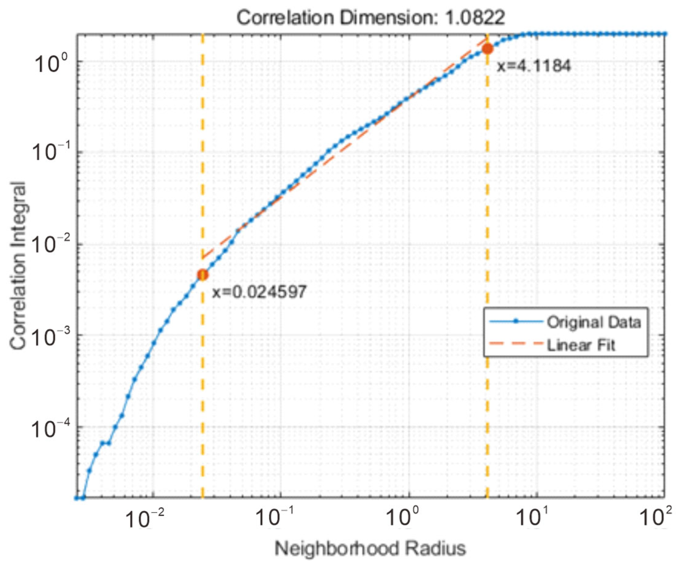
3.2.2. Correlation Dimension Method

The method of calculating the correlation dimension involves the use of a computational approach: delay embedding phase space reconstruction. This study specifically employs the G-P algorithm proposed by Grassberger and Procaccia [51,52]. The correlation dimension also characterizes nonlinear systems in the phase space and describes the self-similarity of signals.

Firstly, the time delay and embedding dimension of the data need to be determined. The delay time τ determines the interval between vector points, while the embedding dimension m determines the length of the vectors. The autocorrelation method is used to calculate the autocorrelation function C(τ) of the time series. When C(τ) is less than ${\displaystyle \frac{C\left(0\right)}{e}}$ (e is the natural logarithm), the corresponding τ is considered the optimal delay time. The formula is as follows:

$$C\left(\tau \right)={\displaystyle \frac{1}{N}}\sum _{i=1}^{n-\tau }x\left(i\right)·x\left(i+\tau \right)$$

(5)

where n represents the number of data points and τ denotes the delay time.

The embedding dimension is determined using the false nearest neighbor (FNN) method. The data are reconstructed, and the results of the vector space reconstruction are as follows:

$$y_t=\left\{x_t,x_{t+\tau },···,x_{t+\left(m-1\right)\tau }\right\}$$

(6)

For each point y_t, its nearest neighbor point y_k is found in the m-dimensional vector space. The formula for the Euclidean distance ratio between the m-dimensional and (m + 1) dimensional vector spaces is as follows:

$$R_d={\displaystyle \frac{\sqrt{\sum _i^{m+1}{\left(y_t^{\left(i\right)}-y_k^{\left(i\right)}\right)}^2}}{\sqrt{\sum _i^m{\left(y_t^{\left(i\right)}-y_k^{\left(i\right)}\right)}^2}}}$$

(7)

where R_d represents the distance variation ratio and m denotes the embedding dimension. If R_d exceeds the set threshold (usually set to 10), the point will be flagged as a false nearest neighbor.

The optimal embedding dimension m is determined by gradually increasing the dimension until the number of false nearest neighbors is minimized. Using the delay time and embedding dimension calculated with the above method, the data are transformed into an m-dimensional vector space. The constructed vector space is as follows:

$$y_i=\left\{x_t,x_{t+\tau },···,x_{t+\left(m-1\right)\tau }\right\},\left(i=1,2,···,N-\left(m-1\right)\tau \right)$$

(8)

The Euclidean distance between any two vectors in the aforementioned vector space is then calculated. Assuming that any two vectors in the embedded space are denoted as y_i and y_j (i, j = 1, 2, ..., K), the formula for calculating their Euclidean distance R_ij is as follows:

$$R_{ij}=\left|y_i-y_j\right|=\sqrt{\sum _{k=1}^N{\left(x_{k+\left(i-1\right)\tau }-x_{k+\left(j-1\right)\tau }\right)}^2}$$

(9)

For an arbitrarily given scale ξ, let N(ξ) represent the number of distances satisfying R_ij < ξ (where i ≠ j), and let the number of vectors be K = N − (m − 1)τ. The total number of distances is K (K − 1). The correlation integral is defined as the ratio of the number of distances meeting the condition R_ij < ξ to the total number of distances.

$$C\left(\xi \right)={\displaystyle \frac{N\left(\xi \right)}{K\left(K-1\right)}}$$

(10)

The method of calculating C(ξ) is as follows:

$$C\left(\xi \right)={\displaystyle \frac{1}{K\left(K-1\right)}}\sum _{i=1}^K\sum _{j=1}^K\theta \left(\xi -R_{ij}\right)\left(i\ne j\right)$$

(11)

$$\mathsf{\theta }\left(\xi -R_{ij}\right)=\left\{\begin{array}{c}0,\text{when} \xi -R_{ij}<0\\ 1,\text{when} \xi -R_{ij}\ge 0\end{array}\right.$$

(12)

The formula for calculating the correlation dimension is as follows:

$$\mathrm{D}=\underset{\xi \to 0}{\lim }{\displaystyle \frac{\log C\left(\xi \right)}{\log \xi }}$$

(13)

Similarly to the box dimension, the slope is generally used to replace the correlation dimension in practical applications. The fractal dimension expresses the self-similarity of data complexity, which can be well used to judge the changes of well logging curves caused by the non-homogeneity of a pore structure.

Figure 5 uses the acoustic log data from well YN4 at 4467–4472 m as an example, creating a plot with the correlation integral and neighborhood radius as the x- and y-axes, respectively. In the plot, the boundaries of the neighborhood radius remain within an approximately linear region. The slope of the fitted line in the plot represents the correlation dimension of the acoustic log.

3.2.3. Multifractal Calculation Based on Wave Leader Method

A multifractal analysis based on the box counting of NMR log data could characterize the properties at each depth. In this study, to describe the heterogeneity of a section of the reservoir, the wave leader method based on one-dimensional logs is utilized. The acoustic and GR logs in the one-dimensional logs are selected as the objects of calculation, with the fractal dimensions of these two logs representing intralayer heterogeneity and microscopic heterogeneity, respectively.

Multifractal computation under the wavelet transform framework primarily involves a multiscale analysis of signals to reveal their complex, non-stationary statistical properties. For a signal X(t₀) that is locally bounded, if there exist a constant C > 0 and a polynomial P satisfying deg(P) < α, then the Hölder exponent at point t₀ is defined as follows [53]:

$$h\left(t_0\right)=sup\left\{a:X\in C^a\left(t_0\right)\right\}$$

(14)

However, directly calculating multifractal properties from the definition of the Hölder exponent is challenging. To address this challenge, the wavelet leader multifractal method employs the wavelet transform as its foundation. This approach shifts the analysis to signal increments and replaces wavelet structural coefficients with local maxima of wavelet transforms. The algorithm offers distinct advantages, including simplified computational procedures and enhanced robustness against noise [54].

Let Ψ₀(t) be a mother wavelet function with compact support. For all $k=0,1,\dots ,N_{\Psi }-1$ satisfies the conditions $\int t^k{\Psi }_0\left(t\right)dt\equiv 0$ and $\int t^{N_{\Psi }}{\Psi }_0\left(t\right)dt\ne 0$, with a vanishing moment $N_{\Psi }\ge 1$. The function set {Ψ_j,k(t)}, generated through the translation and dilation of $\{{\Psi }_{j,k}\left(t\right)=2^{-{\displaystyle \frac{j}{2}}}{\Psi }_0\left(2^{-j}t-k\right),j\in Z,k\in Z\}$, forms an orthonormal basis in L²(R). The discrete wavelet transform (DWT) of a sequence X is defined as follows:

$$d_x\left(j,k\right)=\int {\Psi }_{j,k}X\left(t\right)2^{-j}{\Psi }_0\left(2^{-j}t-k\right)dt$$

(15)

Let $\lambda ={\lambda }_{j,k}=\left[k{2}^j,k\left(k+1\right)2^j\right]$ be defined as a dyadic interval (of scale 2^j), and 3λ be expressed as the union of λ and its two adjacent binary intervals on the same scale j, as specified in Equation (16). Under this constraint, the wavelet leader number expression is as follows:

$${3\lambda }_{j,k}={\lambda }_{j,k-1}\cup {\lambda }_{j,k}\cup {\lambda }_{j,k+1}$$

(16)

$$L_X\left(j,k\right)\equiv L_{\lambda }=\underset{\left[k{2}^j,\left(k+1\right)2^j\right]\subset 3{\lambda }_{j,k}}{\sup }\left|d_X\left(j,k\right)\right|$$

(17)

L_X (j, k) be the maximum wavelet coefficient in the range of 3λ_j,k at all scales, which is used as the wavelet leader number. The scale function (ζ_L) of the structural function (S_L) is calculated through the wavelet leader number, and the calculation formula is as follows:

$$S_L\left(q,j\right)={\displaystyle \frac{1}{n}}\sum _{k-1}^{n_j}{\left|L_X\left(j,k\right)\right|}^q$$

(18)

$${\zeta }_L\left(q\right)=\underset{j\to +\mathrm{\infty }}{\lim \inf }{\displaystyle \frac{\log \left(S_L\left(q,j\right)\right)}{\log \left(2^j\right)}}$$

(19)

Finally, the multifractal spectrum (f(α) − α) can be derived by applying the Legendre transform:

$$\mathsf{\alpha }={\displaystyle \frac{d{\zeta }_L\left(q\right)}{dq}}$$

(20)

$$f\left(\alpha \right)=\underset{q\ne 0}{\inf }\left(1+\alpha -{\zeta }_L\left(q\right)\right)$$

(21)

4. Results and Analysis

4.1. Heterogeneity Analysis Based on Core Permeability

Macroscopic heterogeneities are categorized into interlaminar, intralayer, and lateral heterogeneity, typically resulting from differences in secondary environments, material sources, or geological processes. Interlayer reservoir heterogeneity refers to the macroscopic heterogeneity caused by differences between secondary layers or rock formations. Interlaminar heterogeneity refers to the macroscopic heterogeneity in the horizontal direction within the same sand body segment, describing the geometry, scale, continuity, and variations in porosity and permeability of the reservoir sand body. Intralayer heterogeneity refers to the differences in the vertical direction within the same sandstone layer, including intralayer grain size rhythms and stratification structures, which can also be influenced by thin clay interlayers.

Previous geological studies have shown that the main reservoirs in the DIBEI region consist of braided river delta plain sediments, characterized by poor lateral connectivity within an effective pore space and vertical differences between layers. This study focuses on intralayer heterogeneity, which primarily reflects the changes in the fluid flow capability within individual reservoir units in the vertical direction and is mainly influenced by rock pore structure and discontinuous thin shale layers.

To evaluate intralayer heterogeneity, the core permeability of wells YN2C and YN4 was analyzed using the CV and TK. Figure 6 and Figure 7 present the well logs of wells YN2C and YN4, respectively. In Figure 6, the depth is shown in the first track; the second track presents the natural gamma ray (GR); the third track presents the acoustic (DT), compensated neutron porosity (CNL) and bulk density (DEN) logs; the fourth track presents the resistivity logs, including deep, medium induction resistivity and microsphere-focusing resistivity (Rxo); and the fifth track presents the permeability value obtained from the core experiment. The last track presents the interpretation intervals, including the gas, dry, and water–gas layers. In Figure 7, the fourth track presents the three resistivity curves obtained via array resistivity logging at different measurement depths, and the other curves are the same as those in Figure 6. The two figures have five interpretation intervals based on the well logs, including two dry, one water–gas, and two gas layers. As seen in the figures, the water–gas and dry layers exhibit significantly greater variability in core permeability compared with the gas layers. The CV and TK values of the core permeability of the five intervals are calculated as shown in

Table 2. Parameters of the heterogeneity of core permeability. The fluid types of the intervals were interpreted based on the well logs.

	Dry Layer _1	Water–Gas Layer	Dry Layer _2	Gas Layer _1	Gas Layer _2
Wells	YN4	YN4	YN4	YN2C	YN2C
Thickness (m)	10.5	5.5	8.5	5.9	7.1
Number of data	101	44	88	57	70
MN (mD)	0.57	1.38	0.61	0.65	0.26
MAX (mD)	11.9	9.07	5.61	3.09	1.81
SD	1.51	1.65	0.80	0.68	0.29
TK	20.84	6.56	8.93	4.71	6.84
CV	2.65	1.19	1.32	1.04	1.11
Heterogeneity	Strong	Moderate	Strong	Weak	Weak

. The fluid types of intervals were interpreted based on the well logs.

The results show that the gas layers exhibit the lowest CV and TK values, while the two dry layers have the highest CV and TK values. The CV and TK values of the water–gas layer are in the middle. These values indicate that the dry layers exhibit the strongest heterogeneity and the gas layers exhibit the lowest heterogeneity.

4.2. Fractal Analysis of Well Logs

In the multifractal spectrum, if the f(α)−α spectrum exhibits a unimodal bell-shaped curve and the τ(q)−q relationship deviates from linearity, the signal is confirmed to possess multifractal characteristics. The spectrum width, denoted as Δα, quantifies the heterogeneity of the multifractal structure by measuring the difference between the maximum and minimum singularity exponents. The spectrum width is calculated as follows:

$$∆\alpha ={\alpha }_{max}-{\alpha }_{min}$$

(22)

A larger Δα indicates greater variability in the geological unit’s scaling properties, reflecting a stronger heterogeneity. The natural gamma ray (GR) log reflects rhythmic variations in the sedimentary grain sizes, which are indicative of vertical grain-size distribution patterns, a key manifestation of reservoir heterogeneity. Strong fluctuations in the GR log correlate with great intralayer heterogeneity, making it a robust tool for evaluating intralayer heterogeneity. The multifractal singularity spectrum associated with three types of layers is illustrated in Figure 8. Figure 8a shows the scaling exponent plot, where the three curves are nonlinear convex functions, confirming the multifractal characteristics of the GR log in the three types of layers. If q > 0, large fluctuations play a dominant role, and α(10) is approximately the singularity index corresponding to the maximum fluctuation. If q < 0, small fluctuations play a dominant role, and α(−10) is approximately the singularity index corresponding to the minimum fluctuation. In Figure 8b, the dry layer exhibits a larger interval between α(−10) and α(0), indicating higher variability. Furthermore, the α(−10) value reflects an expanded dynamic range of the log, with more complex small fluctuations in the log. Figure 8c displays the singularity spectrum (f(α) − α), where a broader spectrum width (Δα) signifies greater complexity in lithological variations within the reservoir, directly corresponding to stronger heterogeneity. The multifractal parameters are calculated in

Table 3. Fractal parameters based on the GR logs.

	Dry Layer _1	Water–Gas Layer	Dry Layer _2	Gas Layer _1	Gas Layer _2
Wells	YN4	YN4	YN4	YN2C	YN2C
Thickness (m)	10.5	5.5	8.5	5.9	7.1
Box dimension	1.179	1.138	1.208	1.082	1.081
Correlation dimension	1.401	1.365	1.368	0.917	1.205
Δα	1.480	1.235	1.314	0.958	1.290
α (−10)	2.495	2.162	2.202	1.990	2.094
α (0)	1.385	1.283	1.355	1.617	1.498
α (10)	1.015	0.927	0.888	1.032	0.805
Heterogeneity	Strong	Moderate	Strong	Weak	Weak

. In addition, the fractal and correlation dimensions of GR logs are calculated. As can be seen from Table 3, a strong correlation exists in the three parameters (fractal dimension, correlation dimension, and multifractal spectrum width). The greater the spectrum width, the greater the values of the fractal and correlation dimensions. By comparing the fractal dimensions with the CV and TK values of core permeability, the CV and TK values in those intervals were found to have similar trends to those of the fractal dimension and multifractal spectra. Therefore, the heterogeneity of the gas layer is the weakest, and the heterogeneity of the dry layer is the strongest.

Microscopic heterogeneity is mainly determined by factors such as the pore structure and the interstitial material of the rocks and is mainly related to the size and uniformity of the pore–throats of the rocks, as well as the configuration and connectivity of the pores and throats. In well logging, the acoustic log could indicate the effective porosity, where the response is more pronounced in connected pores. Therefore, acoustic logs were used to characterize the microscopic heterogeneity.

As shown in Figure 9a, the acoustic logs of the three reservoir intervals all exhibit multifractal characteristics. In Figure 9b, the values of parameters for the dry layer are the same as in Figure 8b. In Figure 9c, the width of the singular spectrum of the acoustic log for the dry layer is the largest. The box dimensions, correlation dimensions, and multifractal singular spectrum widths for the three intervals are calculated separately and presented in

Table 4. Fractal parameters based on the acoustic logs.

	Dry Layer _1	Water–Gas Layer	Dry Layer _2	Gas Layer _1	Gas Layer _2
Wells	YN4	YN4	YN4	YN2C	YN2C
Thickness (m)	10.5	5.5	8.5	5.9	7.1
Box dimension	1.158	1.081	1.173	1.108	1.140
Correlation dimension	1.175	1.044	0.975	0.978	1.057
Δα	1.627	1.396	1.728	0.863	0.628
α (−10)	1.956	2.246	1.791	1.825	1.461
α (0)	0.947	1.171	1.037	1.394	1.102
α (10)	0.330	0.850	0.063	0.962	0.833
Heterogeneity	Strong	Moderate	Strong	Weak	Weak

. The three parameters obtained from acoustic logs are consistent with the results obtained from the GR log, that is, the microscopic heterogeneity of the dry layer is the largest, that of the water–gas layer is in the middle, and that of the gas layer is the smallest.

4.3. Correlation Between Heterogeneity and Production

Three wells (YN2C, DB102, and DB101) with varying production capacities were analyzed. Figure 10, Figure 11 and Figure 12 show the well logs, calculated permeabilities, and oil test intervals. To evaluate the relationship between heterogeneity and production, the heterogeneity of the main reservoir sections of wells YN2C, DB102, and DB101 was analyzed using the box counting dimension, correlation dimension, and wavelet leader methods. In these figures, the first track presents the depth; the second track shows the lithology provided by mud logging; the third track presents the lithology analysis data; the fourth track presents the natural gamma ray (GR), caliper (CAL), and bit size (BIT); the fifth track presents the acoustic (DT), compensated neutron porosity (CNL), and density (DEN) logs; the sixth track presents three resistivity curves obtained via array resistivity logging at different measurement depths; the seventh track presents the permeability values calculated from the well logs; the eighth track shows the interpreted intervals, including for the gas and poor gas layers; the ninth track shows the evaluation results of heterogeneity; and the last track is the results of well testing.

Figure 13 and Figure 14 present the calculated multifractal curves of GR and the acoustic logs, respectively. As can be seen from the figures, the calculated results of the two logs share similar characteristics. The scale exponent of Figure 13a and Figure 14a of the three types of reservoirs in both curves is a nonlinear convex function, indicating that the reservoirs have multifractal features. In Figure 13b and Figure 14b, the α(−10) of well DB101 is relatively high, at 1.932 and 2.11 (the first value is from Figure 10, and the second value is from Figure 11), suggesting a high degree of curve fluctuation. Figure 13c and Figure 14c shows the multifractal singularity spectrum. Well DB101 has the widest spectrum, with values of 1.763 and 1.695, while well YN2C has the narrowest, with values of 1.044 and 1.248. In the figures, the values of α(0) − α(10) of the three wells are similar, between 0.4 and 0.7, indicating that the fluctuations in the three wells are similar on a larger scale. The values of α(−10) − α(0) of well DB101 are large, at 1.24 and 1.25, which is related to the small fluctuations in the logging signal, suggesting a high complexity in small fluctuations for the well with low gas production.

The box dimension, correlation dimension, and multifractal spectrum width of the three wells are shown in

Table 5. Fractal parameters of GR logs in three wells.

	YN2C	DB102	DB101
Box dimension	1.228	1.232	1.334
Correlation dimension	1.581	1.686	1.659
Δα	1.044	1.305	1.762
α (−10)	1.691	1.562	1.932
α (0)	1.169	0.908	0.694
α (10)	0.648	0.257	0.169

and

Table 6. Fractal parameters of acoustic logs in three wells.

	YN2C	DB102	DB101
Box dimension	1.130	1.187	1.342
Correlation dimension	1.137	1.079	1.799
Δα	1.248	1.450	1.695
α (−10)	2.165	2.449	2.110
α (0)	1.517	1.667	0.855
α (10)	0.916	1.000	0.414

. The results show that the fractal dimension of wells with high gas production is small, while that of wells with low gas production is large. In Table 5, compared with DB101, DB102 has a higher correlation dimension and box dimension, indicating that DB102 has higher geometric complexity but lower data correlation, whereas DB101 has lower geometric complexity but higher data correlation. In Table 6, the correlation dimension of YN2C is higher than that of DB102, suggesting that the relationship between the acoustic log curves of YN2C and DB102 is the same as the relationship between the GR logs of the aforementioned DB102 and DB101. The data show that YN2C has the highest production and lowest heterogeneity, suggesting that lower heterogeneity may be associated with higher production.

Table 7. Correlation between the multifractal spectrum width and production based on the oil test results.

	YN2C	DB102	DB101
Δα based on GR logs	1.044	1.305	1.763
Δα based on acoustic logs	1.248	1.450	1.695
Oil test (m3/day)	67,320 (gas)	16,328 (gas)	5851 (gas)

summarizes the correlation between the multifractal spectrum width and production based on the oil test results.

The analysis of the three wells showed that, in terms of macroscopic heterogeneity, the values of box dimension, correlation dimension, and multifractal spectrum width indicate that the stronger the heterogeneity, the lower the production. In terms of microscopic heterogeneity, the results from single-fractal calculations show that low productivity and dry layers exhibit similar levels of heterogeneity compared with high gas production zones, but the multifractal analysis reveals that the stronger the heterogeneity, the lower the production.

The fractal and multifractal dimensions of GR and acoustic logs demonstrate that gas reservoirs exhibit low macro- and microscopic heterogeneity compared with dry layers. The geological investigations indicate that the gas reservoirs in well YN2C were deposited in a distributary channel of a braided river delta plain environment, predominantly composed of stable distributary channel microfacies. These channels experienced consistent hydrodynamic conditions during deposition, leading to better sediment sorting and cleaner sandstone layers. In contrast, dry zones and mudstones are associated with floodplain deposits, which contain more interlayers and consequently stronger heterogeneity.

At the microscopic scale, the stable depositional environment of gas reservoirs resulted in quartz grains being less compacted during diagenesis compared with argillaceous particles in dry layers reservoirs. This preserved more regular pore structures, as evidenced by small and uniform variations in the effective porosity on acoustic logs. Consequently, gas reservoirs display lower heterogeneity and smaller fractal dimensions in the acoustic log analysis.

5. Conclusions

Based on core permeability, GR, and acoustic logs, the heterogeneity of a deep tight sandstone reservoir was analyzed using statistical methods and fractal and multifractal theory. The following conclusions are obtained:

(1)

In the analysis of core permeability, the heterogeneity of gas layers is small, and that of dry layers is the largest.

(2)

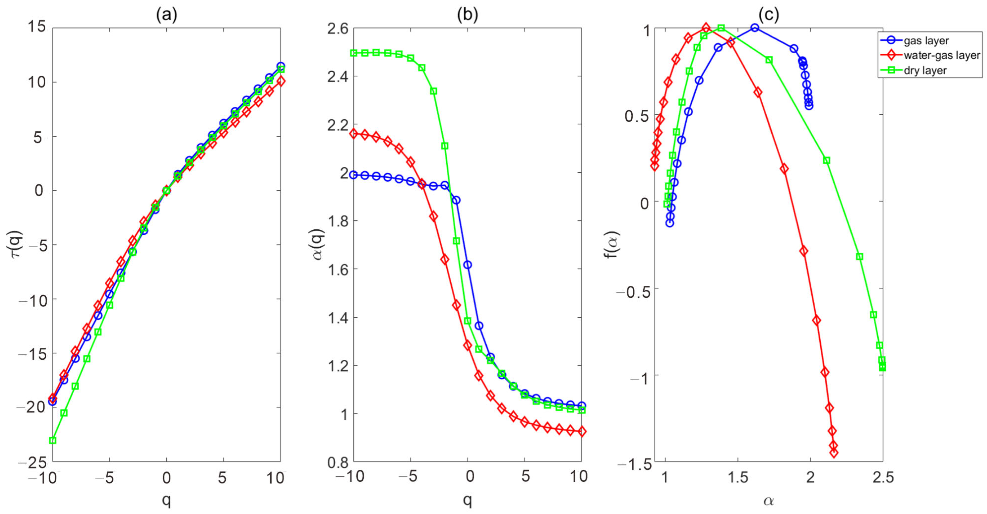
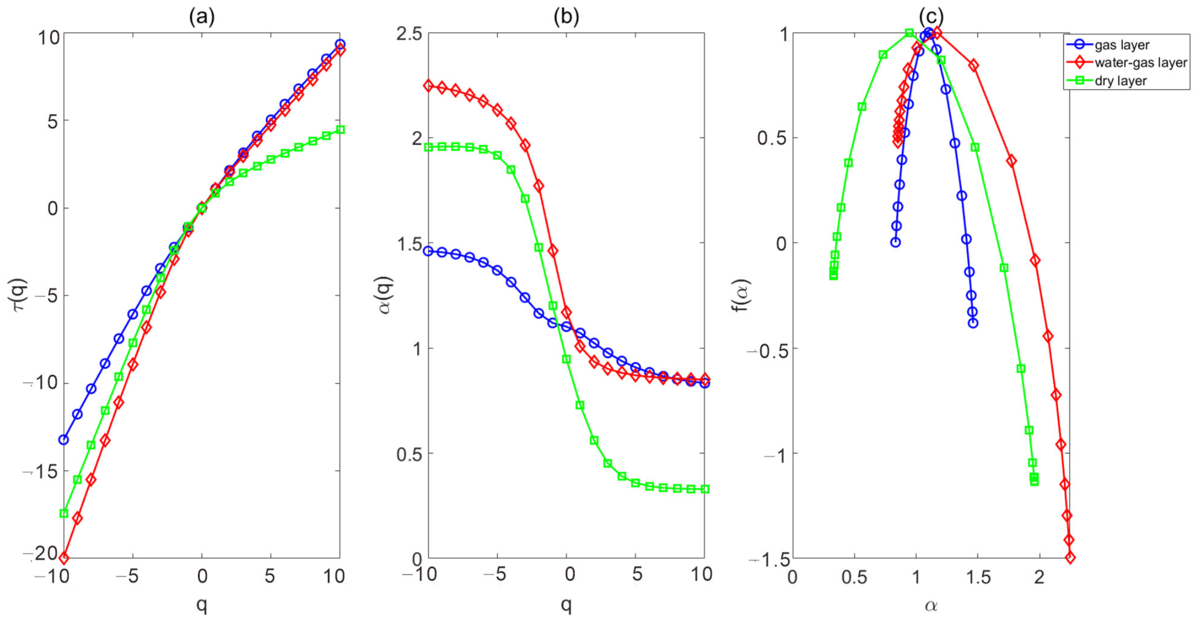
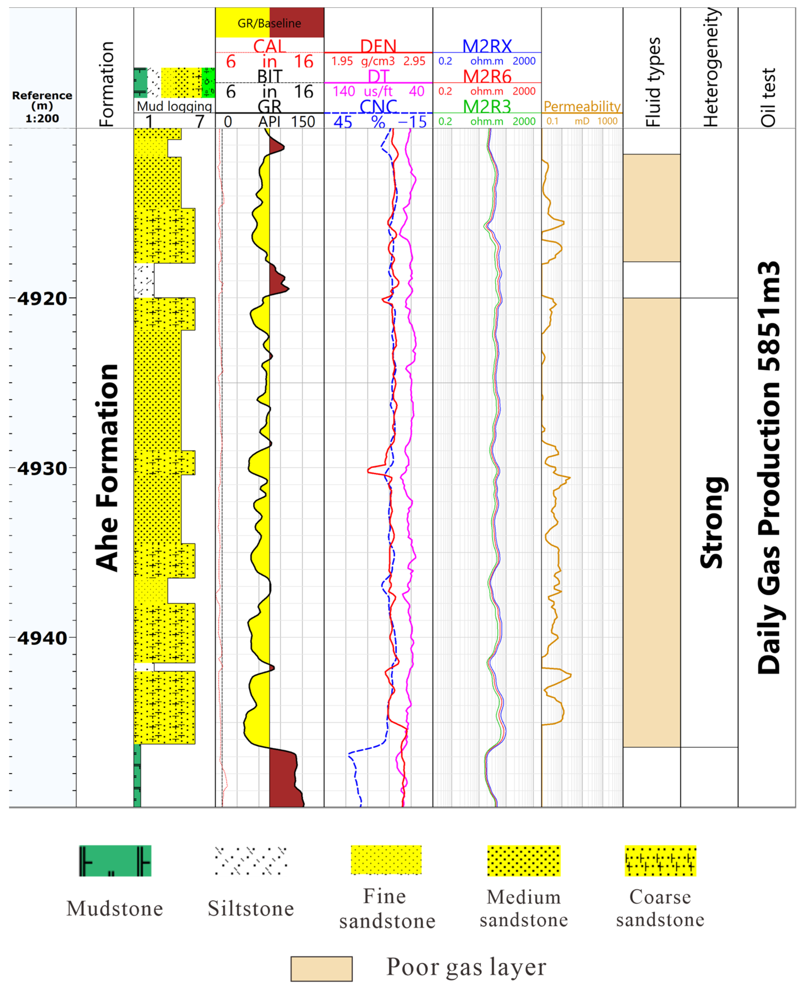
The box dimension, correlation dimension, and multifractal parameter of gas layers, dry layers, and water–gas layers were calculated using well logs. The fractal dimension of the GR log reflects the intralayer heterogeneity within the layer, while the fractal dimension of the acoustic log indicates microscopic heterogeneity. This analysis also examines the two types of heterogeneity in different reservoirs. The two heterogeneity and gas content results were consistent. The calculation results also have good consistency with the results based on core permeability. Layers with high gas content exhibit lower fractal dimensions and weaker heterogeneity, while the dry layers exhibit a larger fractal dimension and stronger heterogeneity.

(3)

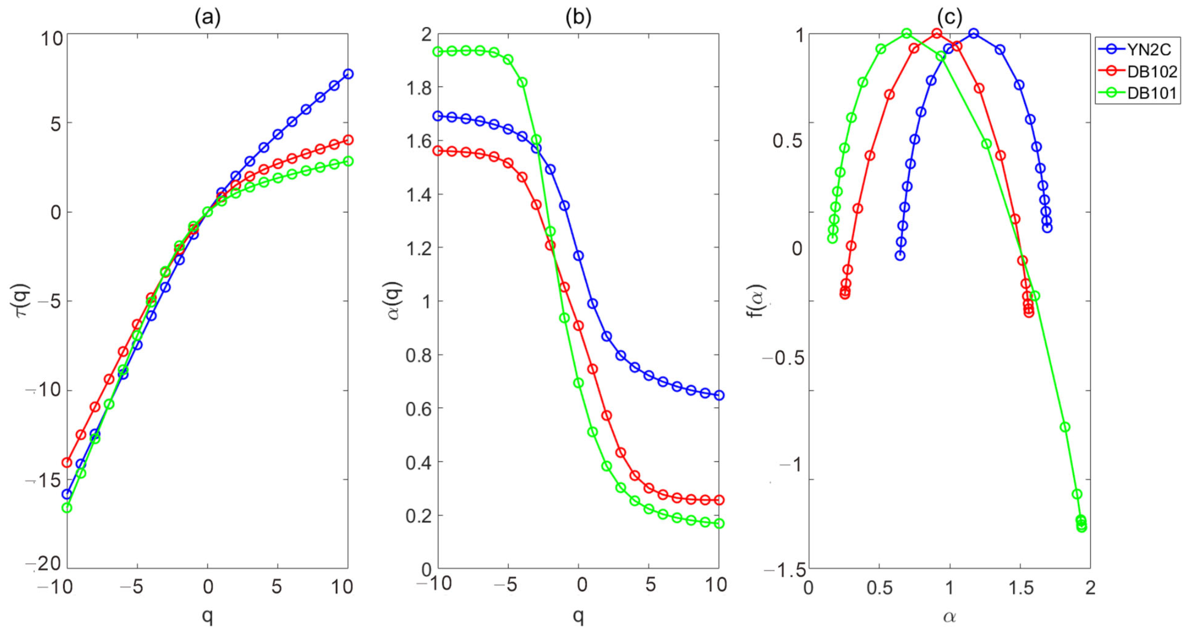
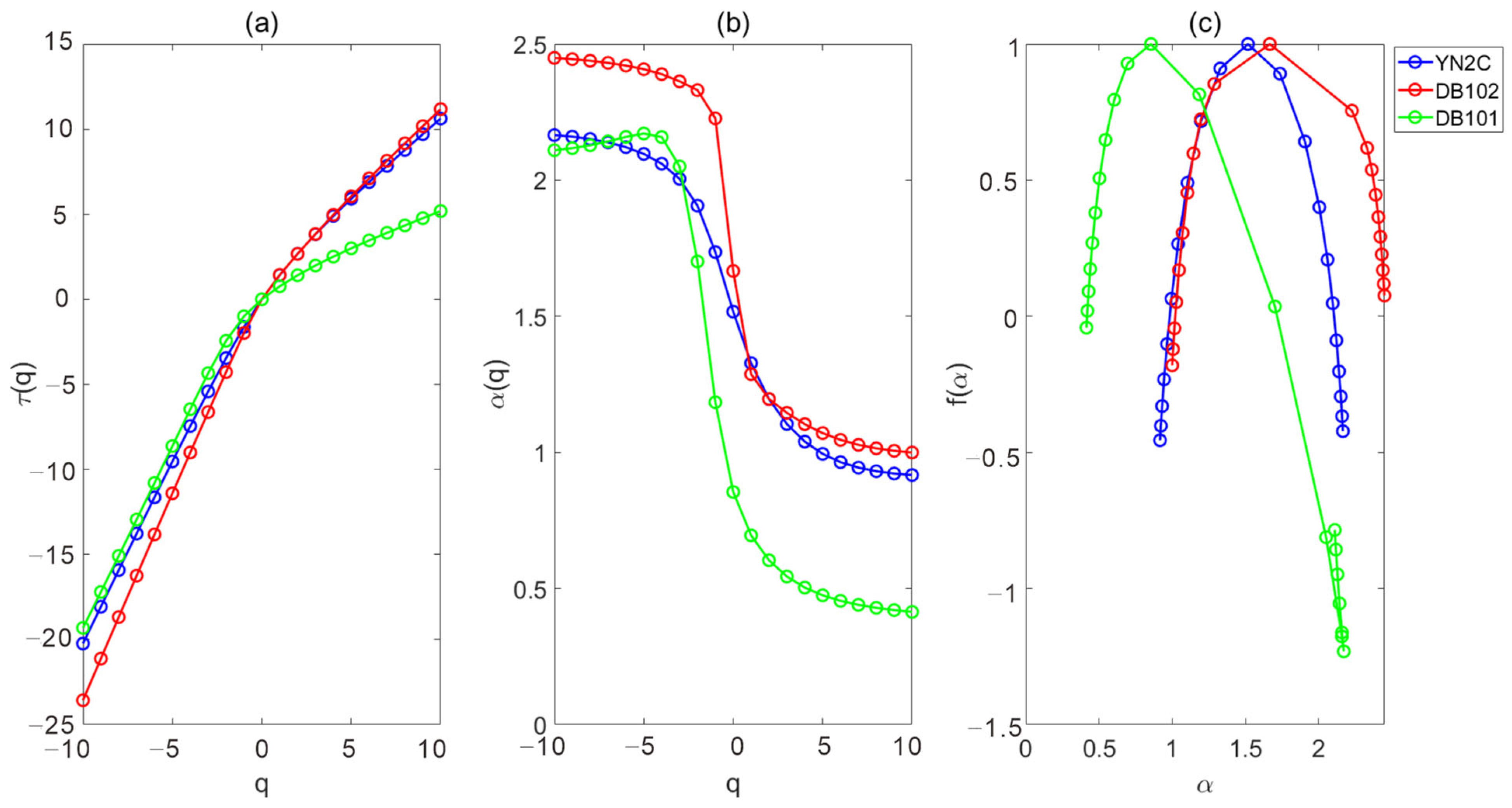
The fractal dimensions and multifractal parameters of the wells with gas production were calculated using GR and acoustic logs, and the heterogeneity of different wells was analyzed. As a result, it was determined that the weaker the heterogeneity, the higher the production. Therefore, the reservoir heterogeneity could be used as an indicator for production estimation.

References

1. Hong, D.; Cao, J.; Wu, T.; Dang, S.; Hu, W.; Yao, S. Authigenic Clay Minerals and Calcite Dissolution Influence Reservoir Quality in Tight Sandstones: Insights from the Central Junggar Basin, NW China. Energy Geosci. 2020, 1, 8–19. [Google Scholar] [CrossRef]
2. Wang, Q.; Yang, H.; Yang, W. New progress and future exploration targets in petroleum geological research of ultra-deep clastic rocks in Kuqa Depression, Tarim Basin, NW China. Pet. Explor. Dev. 2025, 52, 79–94. [Google Scholar] [CrossRef]
3. Wang, G.-X.; Wu, W.; Li, Q.; Liu, W.-Q.; Zhou, Y.-S.; Liang, S.-Q.; Sui, Y.-P. Sequence stratigraphy and sedimentary evolution from Late Cretaceous to Quaternary in the Romney 3D seismic area, deep-water Taranaki Basin (New Zealand). Pet. Sci. 2025, 22, 1854–1875. [Google Scholar] [CrossRef]
4. Tao, K.; Cao, J.; Chen, X.; Nueraili, Z.; Hu, W.; Shi, C. Deep Hydrocarbons in the Northwestern Junggar Basin (NW China): Geochemistry, Origin, and Implications for the Oil vs. Gas Generation Potential of Post-Mature Saline Lacustrine Source Rocks. Mar. Pet. Geol. 2019, 109, 623–640. [Google Scholar] [CrossRef]
5. Mao, Z.; Zeng, L.; Liu, G.; Gao, Z.; Tian, H.; Liao, Q.; Zhang, Y. Fractures and Their Effectiveness in the Deep Jurassic Tight Sandstone Reservoir in the Southern Margin of the Junggar Basin. Pet. Geol. 2020, 41, 1212–1221. [Google Scholar] [CrossRef]
6. Lai, J.; Li, D.; Bai, T.; Zhao, F.; Ai, Y.; Liu, H.; Cai, D.; Wang, G.; Chen, K.; Xie, Y. Reservoir Quality Evaluation and Prediction in Ultra-Deep Tight Sandstones in the Kuqa Depression, China. J. Struct. Geol. 2023, 170, 104850. [Google Scholar] [CrossRef]
7. Wang, J.Y.; Wang, B.; Hu, Z.Q.; Shang, F.; Liu, D.; Li, Z.; Qiu, Q.; Song, Z.; Hu, Z. Genetic Mechanism of High-Quality Reservoirs in Deep-Ultra-Deep Clastic Rocks: A Case Study of the Permian-Triassic in the Central Junggar Basin, NW China. Pet. Nat. Gas Geol. 2025, 46, 151–166. [Google Scholar]
8. Xiao, D.; Lu, S.; Lu, Z.; Huang, W.; Gu, M. Combining Nuclear Magnetic Resonance and Rate-Controlled Porosimetry to Probe the Pore-Throat Structure of Tight Sandstones. Pet. Explor. Dev. 2016, 43, 1049–1059. [Google Scholar] [CrossRef]
9. Schmitt, M.; Fernandes, C.P.; Cunha Neto, J.A.B.; Wolf, G.F. Characterization of Pore Systems in Seal Rocks Using Nitrogen Gas Adsorption Combined with Mercury Injection Capillary Pressure Techniques. Mar. Pet. Geol. 2013, 39, 138–149. [Google Scholar] [CrossRef]
10. Fitch, P.J.; Lovell, M.A.; Davies, S.J.; Pritchard, T.; Harvey, P.K. An Integrated and Quantitative Approach to Petrophysical Heterogeneity. Mar. Pet. Geol. 2015, 63, 82–96. [Google Scholar] [CrossRef]
11. Zheng, C.; Xie, J.; Wang, J.K.; Zhao, X.; Duan, Y.; Sun, Y. Application of Lorenz Coefficient in Reservoir Heterogeneity Evaluation. J. Shandong Univ. Sci. Technol. 2018, 37, 103–110. [Google Scholar] [CrossRef]
12. Lake, L.; Jensen, J. A Review of Heterogeneity Measures Used in Reservoir Characterization. Situ 1991, 15, 409–439. [Google Scholar]
13. Fitch, P.; Davies, S.; Lovell, M.; Pritchard, T. Reservoir Quality and Reservoir Heterogeneity: Petrophysical Application of the Lorenz Coefficient. Petrophysics 2013, 54, 465–474. [Google Scholar]
14. Hosseinzadeh, M.; Tavakoli, V. Analyzing the Impact of Geological Features on Reservoir Heterogeneity Using Heterogeneity Logs: A Case Study of Permian Reservoirs in the Persian Gulf. Geoenergy Sci. Eng. 2024, 237, 212810. [Google Scholar] [CrossRef]
15. Farooq, U.; Ahmed, J.; Ali, S.; Pakistan, M.; Siddiqi, F.; Kazmi, S.A.A.; Mushir, K. Heterogeneity in the Petrophysical Properties of Carbonate Reservoirs in Tal Block. In Proceedings of the SPWLA 60th Annual Logging Symposium, The Woodlands, TX, USA, 15–19 June 2019. [Google Scholar] [CrossRef]
16. Tavoosi, I.P.; Mehrabi, H.; Rahimpour-Bonab, H.; Ranjbar-Karami, R. Quantitative Analysis of Geological Attributes for Reservoir Heterogeneity Assessment in Carbonate Sequences; A Case from Permian–Triassic Reservoirs of the Persian Gulf. J. Pet. Sci. Eng. 2021, 200, 108356. [Google Scholar] [CrossRef]
17. Davies, A.; Cowliff, L.; Simmons, M.D. A Method for Fine-Scale Vertical Heterogeneity Quantification from Well Data and Its Application to Siliciclastic Reservoirs of the UKCS. Mar. Pet. Geol. 2023, 149, 106077. [Google Scholar] [CrossRef]
18. Mandelbrot, B.B. The Fractal Geometry of Nature; W.H. Freeman: San Francisco, CA, USA, 1982. [Google Scholar]
19. Ghanbarian, B.; Hunt, A.G. Fractals: Concepts and Applications in Geosciences; CRC Press: Boca Raton, FL, USA, 2017. [Google Scholar]
20. Jafari, A.; Babadagli, T. Relationship between Percolation–Fractal Properties and Permeability of 2-D Fracture Networks. Int. J. Rock Mech. Min. Sci. Géoméch. Abstr. 2013, 60, 353–362. [Google Scholar] [CrossRef]
21. Pia, G.; Sanna, U. An Intermingled Fractal Units Model to Evaluate Pore Size Distribution Influence on Thermal Conductivity Values in Porous Materials. Appl. Therm. Eng. 2014, 65, 330–336. [Google Scholar] [CrossRef]
22. Karimpouli, S.; Tahmasebi, P. 3D Multi-Fractal Analysis of Porous Media Using 3D Digital Images: Considerations for Heterogeneity Evaluation. Geophys. Prospect. 2019, 67, 1082–1093. [Google Scholar] [CrossRef]
23. Billi, A.; Storti, F. Fractal Distribution of Particle Size in Carbonate Cataclastic Rocks from the Core of a Regional Strike-Slip Fault Zone. Tectonophysics 2004, 384, 115–128. [Google Scholar] [CrossRef]
24. Xie, S.; Cheng, Q.; Ling, Q.; Li, B.; Bao, Z.; Fan, P. Fractal and Multifractal Analysis of Carbonate Pore-Scale Digital Images of Petroleum Reservoirs. Mar. Pet. Geol. 2010, 27, 476–485. [Google Scholar] [CrossRef]
25. Xia, W.; Xi, K.; Xin, H.; Ma, W.; Zhao, H.; Feng, S.; Dan, W. The Influence of Pore Throat Heterogeneity and Fractal Characteristics on Reservoir Quality: A Case Study of Chang 8 Member Tight Sandstones, Ordos Basin. Unconv. Resour. 2025, 5, 100123. [Google Scholar] [CrossRef]
26. Liu, H.; Roquete, M.; Kou, S.; Lindqvist, P.-A. Characterization of Rock Heterogeneity and Numerical Verification. Eng. Geol. 2004, 72, 89–119. [Google Scholar] [CrossRef]
27. Liu, P.; Yuan, Z.; Li, K. An Improved Capillary Pressure Model Using Fractal Geometry for Coal Rock. J. Pet. Sci. Eng. 2016, 145, 473–481. [Google Scholar] [CrossRef]
28. Zhou, Y.; Xu, J.; Lan, Y.; Zi, H.; Cui, Y.; Chen, Q.; You, L.; Fan, X.; Wang, G. New Insights into Pore Fractal Dimension from Mercury Injection Capillary Pressure in Tight Sandstone. Geoenergy Sci. Eng. 2023, 228, 212059. [Google Scholar] [CrossRef]
29. Liu, Y.; Pang, X.Q.; Ding, C.; Chen, D.; Li, M. Pore Structure and Fractal Characteristics of Tight Sandstone Reservoirs in Yan 10 Member of Wuqi Area. Sci. Technol. Eng. 2023, 23, 12474–12483. [Google Scholar]
30. Peng, J.; Han, H.; Xia, Q.; Li, B. Fractal Characteristic of Microscopic Pore Structure of Tight Sandstone Reservoirs in Kalpintag Formation in Shuntuoguole Area, Tarim Basin. Pet. Res. 2020, 5, 1–17. [Google Scholar] [CrossRef]
31. Liu, Y.; Liu, Y.; Zhang, Q.; Li, C.; Feng, Y.; Wang, Y.; Xue, Y.; Ma, H. Petrophysical Static Rock Typing for Carbonate Reservoirs Based on Mercury Injection Capillary Pressure Curves Using Principal Component Analysis. J. Pet. Sci. Eng. 2019, 181, 106175. [Google Scholar] [CrossRef]
32. Wen, H.M. Research on Fractal Well Logging Interpretation Theory and Methods. Ph.D. Thesis, Chengdu University of Technology, Chengdu, China, 2003. [Google Scholar]
33. Mou, D.; Wang, Z.W. Fractal Dimension of Well Logging Curves Associated with the Texture of Volcanic Rocks. In Proceedings of the Industrial and Control Engineering. Ind. Control. Eng. 2014, 278–281. [Google Scholar] [CrossRef]
34. Zhao, P.; Wang, Z.; Sun, Z.; Cai, J.; Wang, L. Investigation on the Pore Structure and Multifractal Characteristics of Tight Oil Reservoirs Using NMR Measurements: Permian Lucaogou Formation in Jimusaer Sag, Junggar Basin. Mar. Pet. Geol. 2017, 86, 1067–1081. [Google Scholar] [CrossRef]
35. Yan, J.-P.; He, X.; Geng, B.; Hu, Q.-H.; Feng, C.-Z.; Kou, X.-P.; Li, X.-W. Nuclear magnetic resonance T2 spectrum multifractal characteristics and pore structure evaluation. Appl. Geophys. 2017, 14, 205–215. [Google Scholar] [CrossRef]
36. Zhao, P.; Wang, X.; Cai, J.; Luo, M.; Zhang, J.; Liu, Y.; Rabiei, M.; Li, C. Multifractal Analysis of Pore Structure of Middle Bakken Formation Using Low Temperature N2 Adsorption and NMR Measurements. J. Pet. Sci. Eng. 2019, 176, 312–320. [Google Scholar] [CrossRef]
37. Lv, H.; Guo, J.; Gu, B.; Zhu, Z.; Zhang, Z. A Fracture Identification Method Using Fractal Dimension and Singular Spectrum Entropy in Array Acoustic Logging: Insights from the Asmari Formation in the M Oilfield, Iraq. J. Appl. Geophys. 2025, 233, 105631. [Google Scholar] [CrossRef]
38. Lozada-Zumaeta, M.; Arizabalo, R.; Ronquillo-Jarillo, G.; Coconi-Morales, E.; Rivera-Recillas, D.; Castrejón-Vácio, F. Distribution of Petrophysical Properties for Sandy-Clayey Reservoirs by Fractal Interpolation. Nonlinear Process. Geophys. 2012, 19, 239–250. [Google Scholar] [CrossRef]
39. Partovi, S.M.A.; Sadeghnejad, S. Fractal Parameters and Well-Logs Investigation Using Automated Well-to-Well Correlation. Comput. Geosci. 2017, 103, 59–69. [Google Scholar] [CrossRef]
40. López, M.; Aldana, M. Facies Recognition Using Wavelet Based Fractal Analysis and Waveform Classifier at the Oritupano-A Field, Venezuela. Nonlinear Process. Geophys. 2007, 14, 325–335. [Google Scholar] [CrossRef]
41. Subhakar, D.; Chandrasekhar, E. Reservoir Characterization Using Multifractal Detrended Fluctuation Analysis of Geophysical Well-Log Data. Stat. Mech. Its Appl. 2016, 445, 57–65. [Google Scholar] [CrossRef]
42. Amoura, S.; Gaci, S.; Barbosa, S.; Farfour, M.; Bounif, M. Investigation of Lithological Heterogeneities from Velocity Logs Using EMD-Hölder Technique Combined with Multifractal Analysis and Unsupervised Statistical Methods. J. Pet. Sci. Eng. 2022, 208, 109588. [Google Scholar] [CrossRef]
43. Prajapati, R.; Kumar, R.; Singh, U.K. Assessment of Reservoir Heterogeneities and Hydrocarbon Potential Zones Using Wavelet-Based Fractal and Multifractal Analysis of Geophysical Logs of Cambay Basin, India. Mar. Pet. Geol. 2024, 160, 106633. [Google Scholar] [CrossRef]
44. Wang, Q.H.; Zhang, R.H.; Yang, X.Z.; Chen, X.; Xiao, D.; Wang, B.; Wu, C.; Yu, H. Major Breakthrough and Geological Significance of Tight Sandstone Gas Ex-ploration in Jurassic Ahe Formation of Dibei Area, Eastern Kuqa Depression. Acta Pet. Sinica. 2022, 43, 1049–1064. [Google Scholar] [CrossRef]
45. Zhao, M.J.; Zhang, S.C. Genetic Types and Accumulation Conditions of Natural Gas in Tarim Basin. China Pet. Explor. 2001, 6, 27–31. [Google Scholar]
46. Wei, G.; Wang, K.; Zhang, R.; Wang, B.; Yu, C. Structural Diagenesis and High-Quality Reservoir Prediction of Tight Sandstones: A Case Study of the Jurassic Ahe Formation of the Dibei Gas Reservoir, Kuqa Depression, Tarim Basin, NW China. J. Asian Earth Sci. 2022, 239, 105399. [Google Scholar] [CrossRef]
47. Yang, Y.-B.; Xiao, W.; Zheng, L.-L.; Lei, Q.-H.; Qin, C.-Z.; He, Y.-A.; Liu, S.-S.; Li, M.; Li, Y.-M.; Zhao, J.-Z.; et al. Pore Throat Structure Heterogeneity and Its Effect on Gas-Phase Seepage Capacity in Tight Sandstone Reservoirs: A Case Study from the Triassic Yanchang Formation, Ordos Basin. Pet. Sci. 2023, 20, 2892–2907. [Google Scholar] [CrossRef]
48. Liang, D.G.; Jia, C.Z. Achievements and Prospect Prediction of Natural Gas Exploration in Tarim Basin. Nat. Gas Ind. 1999, 19, 3–12. [Google Scholar]
49. Li, D.; Wang, G.; Bie, K.; Lai, J.; Lei, D.-W.; Wang, S.; Qiu, H.-H.; Guo, H.-B.; Zhao, F.; Zhao, X.; et al. Formation Mechanism and Reservoir Quality Evaluation in Tight Sandstones under a Compressional Tectonic Setting: The Jurassic Ahe Formation in Kuqa Depression, Tarim Basin, China. Pet. Sci. 2024, 22, 998–1020. [Google Scholar] [CrossRef]
50. Hu, H.; Wang, G.C.; Wang, Y.Z.; Huang, R. Yan’an Oilfield Fuchang Development Unit Chang 2 Heterogeneity Study. J. Hebei GEO Univ. 2024, 47, 34–42. [Google Scholar] [CrossRef]
51. Grassberger, P.; Procaccia, I. Measuring the Strangeness of Strange Attractors. Nonlinear Phenom. 1983, 9, 189–208. [Google Scholar] [CrossRef]
52. Liao, Z.; Wang, L.; He, Z. Feature Extraction and Classification of Mining Microseismic Signals Based on EEMD and Correlation Dimension. Gold Sci. Technol. 2020, 28, 585–594. [Google Scholar]
53. Tan, Z.; Huang, J.; Ye, C. Identification of major turning points in the Chinese stock market: A Bayesian approach based on improved wavelet leader method and approximation techniques. China Manag. Sci. 2018, 26, 12–24. [Google Scholar] [CrossRef]
54. Zhang, L.; Li, R.J.; Liu, X.L. Analysis of Stock Market Effectiveness and Risk Detection Based on Wavelet Leader Multifractal Method. Chin. J. Manag. Sci. 2014, 22, 17–26. [Google Scholar]
Figure 3. Distribution of porosity and permeability in the Dibei area. (a) Porosity distribution histogram; (b) Permeability distribution histogram.
Fractalfract 09 00431 g003
Figure 4. The cross-plot of box dimension calculations.
Fractalfract 09 00431 g004
Figure 5. The cross-plot of correlation dimension calculation.
Fractalfract 09 00431 g005
Figure 6. Conventional logs and core permeability in the water–gas and dry layers.
Fractalfract 09 00431 g006
Figure 7. Conventional logs and core permeability in the gas layers.
Fractalfract 09 00431 g007
Figure 8. Multifractal characteristics of the GR logs of three types of layers in YN4 and YN2C: (a) variation in the scaling coefficient with q order; (b) variation in the Hurst index with q order; and (c) multifractal singular spectrum of three types of reservoirs. The values of ∆α are 0.958 in the gas layer and 1.48 in the dry layer, while α(0) is 1.385 in the gas layer and 1.498 in the dry layer, respectively.
Fractalfract 09 00431 g008
Figure 9. Multifractal characteristics of the acoustic log curves: (a) variation in the scale coefficient with q order; (b) variation in the Hurst index with q order; and (c) multifractal singular spectrum of three types of reservoirs. The values of ∆α are 0.863 in the gas layer and 1.627 in the dry layer, while α(0) is 1.394 in the gas layer and 0.947 in the dry layer, respectively.
Fractalfract 09 00431 g009
Figure 10. Analysis of the heterogeneity and results of oil testing in well YN2C.
Fractalfract 09 00431 g010
Figure 11. Analysis of the heterogeneity and results of oil testing in well DB102.
Fractalfract 09 00431 g011
Figure 12. Analysis of the heterogeneity and results of oil testing in well DB101.
Fractalfract 09 00431 g012
Figure 13. Results of the GR log calculations in three wells: (a) variation in the scaling coefficient with q order; (b) variation in the Hurst index with q order; and (c) multifractal singular spectrum of three types of gas layers. The values of ∆α are 1.044 in well YN2C and 1.763 in well DB101, while α(0) is 1.169 and 0.694, respectively.
Fractalfract 09 00431 g013
Figure 14. Results of the acoustic log calculations in three wells: (a) variation in the scale coefficient with q order; (b) variation in the Hurst index with q order; and (c) multifractal singular spectrum of three types of gas layers. The values of ∆α are 1.248 in well YN2C and 1.695 in well DB101, while α(0) is 1.517 and 0.855, respectively.
Fractalfract 09 00431 g014