Comparative Evaluation of Fractional-Order Models for Lithium-Ion Batteries Response to Novel Drive Cycle Dataset

Abstract

The high-fidelity lithium-ion battery (LIB) models are crucial for realizing an accurate state estimation in battery management systems (BMSs). Recently, the fractional-order equivalent circuit models (FOMs), as a frequency-domain modeling approach, offer distinct advantages for constructing high-precision battery models in field of electric vehicles. However, the quantitative evaluations and adaptability of these models under different driving cycle datasets are still lacking and challenging. For this reason, comparative evaluations of different FOMs using a novel drive cycle dataset of a battery was carried out in this paper. First, three typical FOMs were initially established and the particle swarm optimization algorithm was then employed to identify model parameters. Complementarily, the efficiency and accuracy of the offline identification for three typical FOMs are also discussed. Subsequently, the terminal voltages of these different FOMs were investigated and evaluated under dynamic operating conditions. Results demonstrate that the FOM-W model exhibits the highest superiority in simulation accuracy, achieving a mean absolute error (MAE) of 9.2 mV and root mean square error (RMSE) of 19.1 mV under Highway Fuel Economy Test conditions. Finally, the accuracy verification of the FOM-W model under two other different dynamic operating conditions has also been thoroughly investigated, and it could still maintain a RMSE and MAE below 21 mV, which indicates its strong adaptability and generalization compared with other FOMs. Conclusions drawn from this paper can further guide the selection of battery models to achieve reliable state estimations of BMS.

1. Introduction

Recently, electrochemical energy storage has been recognized as a leading high-energy storage technology, with widespread application in electric vehicles (EVs), power grids, and consumer electronics [1]. With the strong deployment of the dual carbon policy, lithium batteries (LIBs) have garnered significant attention within the EV sector, largely because they offer high energy density, a low self-discharge rate, and prolonged operational life [2,3]. However, the effective monitoring of battery status by battery management systems (BMS) still faces challenges as people’s safety awareness increases. Given that the precise battery model can capture battery dynamics across varied operational scenarios, it is crucial for real-time monitoring of state of charge (SOC) and state of health (SOH) in practical applications of EVs [4,5].

According to current research reports, the battery model is generally classified into three categories: electrochemical model (EM), data-driven model (DDM), and equivalent circuit model (ECM) [6,7]. From a physicochemical point of view, the EM can accurately characterize chemical and physical reactions through partial differential equations describing ion diffusion, migration, and electrode kinetics [8]. Unfortunately, neither the pseudo-two-dimensional model nor the more simplified single-particle model can avoid complex parameter identification and high computing cost [9,10,11], which significantly increases challenges in term of real-time application requirements. In comparison, the DDM [12,13] mainly analyzes collected battery data to identify nonlinear dynamic characteristics for modeling and state estimation. Specifically, the DDMs usually employ machine learning methods (e.g., neural networks [14,15]) to establish nonlinear mappings between battery inputs and outputs through extensive experimental data training. Especially when internal battery mechanisms are insufficiently characterized, this method is proved to be particularly effective [16,17]. Nevertheless, DDMs still exhibit inherent limitations in the following two aspects: the prediction performance heavily depends on training data quality and quantity, and poor generalization capability restricts practical applications across diverse battery types and operational scenarios [18].

Different from battery models mentioned above, ECMs are the most widely used method in engineering practice owing to their straightforward structure and ease of parameter identification [19]. It is reported that this model is usually composed of ideal resistors, capacitors, and voltage sources so that it can simulate the battery’s current–voltage characteristics [20]. Nevertheless, Freeborn T J et al. discovered that conventional ECMs exhibit limited efficacy in fitting the low-frequency impedance characteristics of LIBs [21]. To address this issue, Yu et al. developed a fractional-order equivalent circuit model (FOM) by incorporating a constant phase element (CPE) [22]. And empirical evidence has demonstrated that FOM can more accurately describe impedance spectrum characteristics of batteries in the medium- and low-frequency regions. In addition, Chen et al. compared the parameter identification results of FOMs and ECMs using the recursive least squares method, and it demonstrates that the FOMs can effectively eliminate the disadvantage of ECMs and present higher performance advantages in accuracy [23]. More excitingly, this conclusion has also been further verified in various published researches, and FOMs have been gradually employed for the estimation of battery SOC and SOH [24,25,26]. Moreover, compared to EMs and DDMs, the FOMs also exhibit significantly reduced complexity and better conformity with actual physical processes, which makes FOMs hold considerable application prospects in the monitoring and management of LIBs [27].

It is worth noting that the selection of structures in FOMs inevitably affects voltage response characteristics. In this regard, Tian et al. compared five FOMs from the perspective of SOC estimation and pointed out that complexity of the FOMs may not be proportional to its simulation accuracies [28]. Subsequently, Wang et al. carried out the in-depth comparison in voltage accuracy and parameter identification efficiency for four typical FOMs [29]. Recently, Tian et al. also summarized battery modeling methods of FOMs and explored the differences in model discretization [30]. For parameter benchmark, Meng et al. innovatively evaluated the efficacy of offline parameter identification methods for ECMs across diverse operating conditions [31]. Although the above studies extensively studied the impact of model structures on accuracy, there are still limitations. For instance, the parameter identification efficiency of different FOMs can be further refined. And the driving cycle dataset for model adaptability is not rich and cannot fully cover the battery operation status in vehicle scenarios. More importantly, the evaluation and comparisons of FOMs under these conditions are not systematically discussed.

Responding to the above issues, a comparative evaluation of different FOMs for LIB responses to the novel drive cycle dataset is carried out in this paper. Firstly, the fractional-order differential theory is introduced, and the construction of three FOMs is explored. Subsequently, the particle swarm optimization (PSO) algorithm-based parameters identification for different FOMs is investigated. Complementarily, efficiency for offline identification under the same operating scenario is summarized. Furthermore, the accuracies of three FOMs are also validated and compared under collected drive cycle conditions. Ultimately, the optimal model is further evaluated for adaptability using more dynamic datasets. The main contributions of this paper can be outlined as follows:

• PSO-based parameter identification for three FOMs are systematically compared.
• Voltage responses of three FOMs under drive cycle conditions are evaluated and discussed.
• The optimal model’s adaptability under more dynamic conditions are further investigated.

The remainder of the paper is organized as follows: Section 2 gives methodology of the FOMs, and results and discussion are presented in Section 3. Finally, the conclusions are given in Section 4.

2. Fractional-Order Battery Modeling

The traditional RC model requires additional RC networks to enhance accuracy, which inevitably introduces parameter redundancy and obscures the physical interpretation [32]. In contrast, by incorporating fractional-order theory, the FOM not only achieves comparable accuracy but also retains model simplicity, thereby effectively overcoming these limitations of integer-order models. Therefore, the basic theory and methodology of the FOM modeling for comparative evaluation are given in this section.

2.1. Theory of Fractional-Order Models

FOMs provide more accurate physical system descriptions than their integer-order counterparts. Among existing fractional-order definitions, including Riemann–Liouville (R-L), Caputo, and Oustaloup’s approximation, each suited to different applications, the Grünwald–Letnikov (G-L) definition [33] is adopted herein. As a direct extension of classical integer-order calculus, the inherent simplicity and ease of use of the G-L method are highly effective for establishing FOMs of batteries and implementing their numerical calculations. The formula can be presented as follows:

$$D_c^{\alpha }f(t)=\left\{\begin{array}{l}{\displaystyle \frac{d^{\alpha }}{d{t}^{\alpha }}}f(t),\hspace{1em}\hspace{1em}\alpha >0\\ f(t),\hspace{1em}\hspace{1em}\hspace{1em} \alpha =0\\ {\displaystyle {\int }_c^{t}f(t)d{\tau }^{\alpha },\hspace{1em} \alpha <0}\end{array}\right.$$

(1)

where $\alpha \in R$, the term $D_c^{\alpha }$ denotes the fractional-order integral if $\alpha <0$, and it signifies the fractional-order differential if $\alpha >0$. The constant $c\in R$ serves as the lower integration boundary, physically corresponding to the starting time. Within the scope of this research, the system’s initial time is established as zero, meaning $c=0$.

In addition, for any given function $f(t)$, its G-L definition for a fractional order $\alpha$ is given by the following [34]:

$$D_c^{\alpha }f(t)=\underset{\Delta T\to 0}{\lim }{\displaystyle \frac{1}{\Delta T^{\alpha }}}{\displaystyle \sum _{i=0}^{\left[t/\Delta T\right]}{(-1)}^i}\left(\begin{array}{c}\alpha \\ i\end{array}\right)f(t-i\Delta T)$$

(2)

In this equation, $\Delta T$ denotes the sampling interval; the term $\left[t/\Delta T\right]$ represents the integral component of the ratio $t/\Delta T$. Furthermore, it should be noted that $\left(\begin{array}{c}\alpha \\ i\end{array}\right)$, representing the Newtonian binomial coefficient, is defined as follows:

$$\left(\begin{array}{c}\alpha \\ i\end{array}\right)={\displaystyle \frac{\alpha !}{i!(\alpha -1)!}}={\displaystyle \frac{\Gamma (\alpha +1)}{\Gamma (i+1)\Gamma (\alpha -i+1)}}$$

(3)

2.2. Fractional-Order Model of the Battery

In order to further use fractional-order theory for model construction, the electrochemical impedance technology (EIS) is briefly discussed here. It is reported that EIS can been utilized for characterizing the impedance behavior of a battery across different frequency bands. And the prerequisite for realizing this function requires applying a small-amplitude sinusoidal current perturbation over a wide frequency range. A typical impedance spectrum for LIB is illustrated in Figure 1, which exhibits distinct frequency regions. These regions are often interpreted and modeled using equivalent circuits composed of resistors, capacitors, and CPE [35]

According to descriptions in the Ref. [36], the high-frequency domain primarily indicates the resistive behavior of the electrolyte and diaphragm, a characteristic linked to the transport of lithium-ions and electrons; this behavior is typically represented by a single resistive component. The mid-frequency semicircle shown in Figure 1 is linked to the charge transfer taking place at the boundary between the electrode and electrolyte and is typically represented using a resistor and a CPE in a parallel arrangement. Moreover, the inclined line observed at lower frequencies stems from the diffusion processes of lithium ions within the solid phase of the active material; an appropriate impedance model for this section is chosen based on particular requirements. For instance, to enhance computational speed, Tian J et al. disregarded the effects from the low-frequency domain [33]. To characterize the low-frequency behavior, Umar A et al. incorporated a Warburg impedance into their model [37]. For an improved representation of the mid-frequency impedance response, Chen L et al. introduced an additional R-CPE parallel circuit to an existing fractional first-order model [23].

Based on the electrochemical principle, the impedance of a CPE is given by the following:

$$Z={\displaystyle \frac{1}{C_{CPE}{S}^{\alpha }}}, 1>\alpha >0$$

(4)

where $C_{CPE}$ is the impedance and $\alpha$ is the fractional order. When $\alpha =1$, CPE is equivalent to a capacitive element, and when $\alpha =0.5$, CPE can be viewed as a Warburg element.

Considering this advantage and the importance of model selection to accurately predict battery performance, this study selects three representative FOMs that differ in complexity and their representation of electrochemical dynamics: a fractional first-order model (called FOM-1) [27], fractional first-order model with Warburg impedance (called FOM-W) [38], and fractional second-order model (called FOM-2) [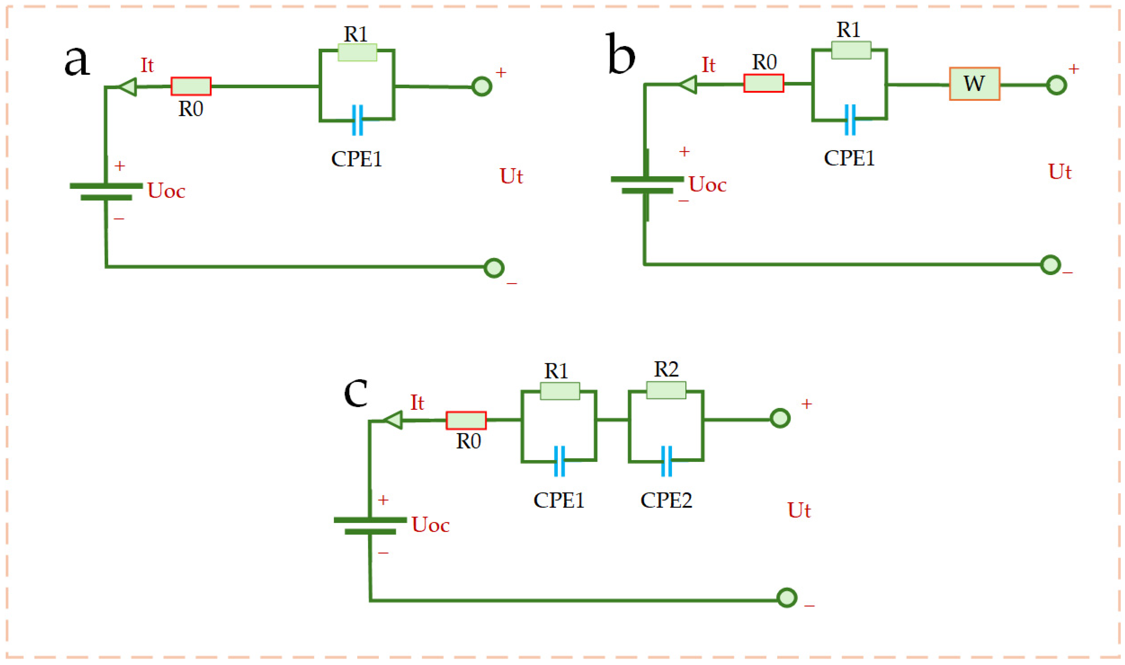39]. And the detailed structure of these models can be found in Figure 2. The specific mathematical derivation and structure of these FOMs will be further described in Section 2.2.1, prior to their comparative evaluation under a novel driving cycle dataset which aims to provide a practical reference for LIB model selection.

2.2.1. FOM-1

As shown in Figure 2a, the FOM-1 architecture comprises an open-circuit voltage (OCV) source, an ohmic resistor R0, and an R-CPE network [6]. To elaborate on its components, within FOM-1, the OCV element primarily serves to model the open-circuit voltage. The resistor R0 is employed to represent the cell’s static behavior, while the R-CPE network is included to better capture the cell’s performance during dynamic operations. A discussion of more structural parameters can be found in Ref. [33].

Applying Kirchhoff’s current and voltage laws, the equations for this single fractional-order RC model are derived as follows:

The expression for the terminal voltage is as follows:

$$V_i=OCV\left(SOC\right)-R_{0}I\left(t\right)-U_1\left(t\right)$$

(5)

The voltage behavior of the R-CPE network is given by the following:

$${\tau }_1{D}^{\alpha }{U}_1(t)+U_1(t)=R_{1}I(t),\hspace{1em}{\tau }_1=R_1{C}_1$$

(6)

The updated formula after G-L discretization can be expressed as follows:

$$U_1(k)=-{\displaystyle \frac{T_s^{\alpha }}{{\tau }_1}}{U}_1(k-1)+{\displaystyle \frac{T_s^{\alpha }}{C_1}}I(k-1)-{\displaystyle \sum _{j=2}^L{w}_{u1}}(j)U_1(k-j+1)$$

(7)

where $T_{\mathrm{s}}$ denotes the sampling interval, $w_{u1}$ represents the weighting coefficient, $L$ signifies the memory length, and $k$ is the discrete time step.

2.2.2. FOM-W

To explain the FOM-W model, its structure can be found in Figure 2b. Specifically, a Warburg element is incorporated in series with FOM-1, traditionally employing a fixed order of 0.5 to represent the model’s diffusion-driven low-frequency behavior [38]. However, in the present work, the Warburg element’s order is treated as an identifiable variable during parameter estimation, granting it a flexibility comparable to that of a CPE. The element’s coefficient and order are denoted by W and γ, respectively.

The voltage behavior of the combined R-W-CPE network is given by the following:

$$V_t=OCV(SOC)-R_0(SOC)\cdot I(t)-U_1(t)-U_w(t)$$

(8)

The voltage characteristics of Warburg components can be expressed as follows:

$$U_w(t)=W\cdot D^{-\gamma }I(t)$$

(9)

The update equation for the Warburg component is given by the following:

$$U_w(k)={\displaystyle \frac{T_s^{\gamma }}{W}}I(k-1)-{\displaystyle \sum _{j=2}^L{w}_{u2}}(j)U_w(k-j+1)$$

(10)

where $U_w(k)$ is the voltage of the Warburg element at a discrete moment k, $W$ represents the Warburg coefficient, and $\gamma$ indicates its fractional order.

The formulation for the weighting factors is as follows:

$$w_{u1}(j)={(-1)}^j{\displaystyle \frac{\Gamma (\alpha +1)}{\Gamma (\alpha -j+1)\Gamma (j+1)}}$$

(11)

2.2.3. FOM-2

To potentially capture more complex battery dynamics than FOM-1, the second-order fractional model (FOM-2) is introduced, as depicted in Figure 2c. This model enhances the FOM-1 structure by incorporating an additional R-CPE network [39].

The equations defining the terminal voltage are formulated as follows:

$$V_t=OCV(SOC)-R_0(SOC)\cdot I(t)-U_1(t)-U_2(t)$$

(12)

The characteristics of the additionally incorporated R-CPE network are described by the following:

$${\tau }_2{D}^{{\alpha }_2}{U}_2(t)+U_2(t)=R_{2}I(t),\hspace{1em}{\tau }_2=R_2{C}_2$$

(13)

The updated formula of the fractional-order R2-CPE2 network after the G-L discretization form is as follows:

$$U_2(k)=-{\displaystyle \frac{T_s^{{\alpha }_2}}{{\tau }_2}}{U}_2(k-1)+{\displaystyle \frac{T_s^{{\alpha }_2}}{C_2}}I(k-1)-{\displaystyle \sum _{j=2}^L{w}_{u2}}(j)U_2(k-j+1)$$

(14)

The weighting factors can be expressed as the following:

$$w_{u2}(j)={(-1)}^j{\displaystyle \frac{\Gamma ({\alpha }_2+1)}{\Gamma ({\alpha }_2-j+1)\Gamma (j+1)}}$$

(15)

2.3. Parameter Identification of FOMs Based on the PSO Algorithm

Within the domain of parameter identification, numerous methodologies have been investigated by researchers, such as the genetic algorithm (GA) and recursive least squares (RLS). Nevertheless, the GA is susceptible to converging at local optima, and the RLS often lacks precision for the highly non-linear characteristics inherent in these FOMs, and the extended Kalman filter (EKF) [30] is often constrained by the high computational cost stemming from the large number of state variables in such FOMs. 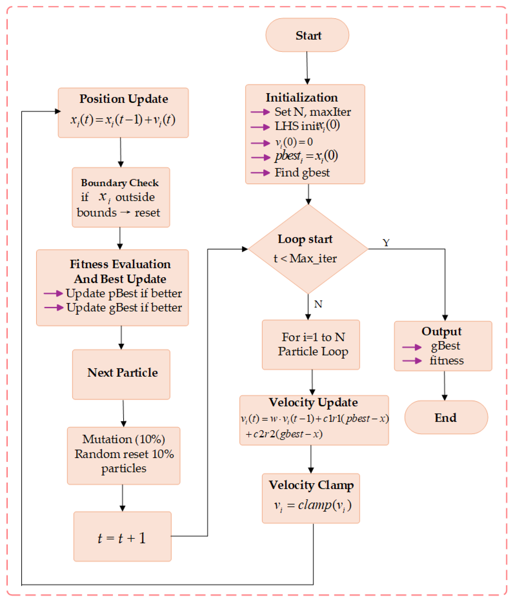In contrast, the PSO algorithm, leveraging its robust global search ability [40], is particularly effective for finding optimal parameter solutions in complex and nonlinear fitting problems, proving highly suitable for the FOMs in this study. Furthermore, Figure 3 illustrates the detailed procedure of its application for determining the FOM parameters.

To facilitate a clearer comprehension of this procedure and the fundamental principles of the selected algorithm for identifying the parameters of the FOMs, a concise overview of PSO is firstly introduced. In general, the PSO functions as a probabilistic optimization method inspired by the collective behavior observed in natural swarms. Although the PSO has certain general limitations, it is more suitable for parameter identification and analysis of different fractional-order models compared with other optimization algorithms. It needs to be emphasized that the algorithm strives to find the optimal FOM parameters by iteratively adjusting particle positions and velocities within a high-dimensional search space corresponding to the FOM parameter domain. The following outlines its primary process steps:

• Step 1. Initialization phase:

This involves defining the swarm (population) size $N$, establishing the upper limit for iterations $Max\_iter$, specifying the permissible range for parameters $\left[lb,ub\right]$ (which correspond to the bounds for each parameter of the FOMs, such as $R_1$, $\tau$, $\alpha$, etc.), and formulating the objective function as indicated below:

$$RMSE=\sqrt{{\displaystyle \frac{1}{n}}{\displaystyle \sum _{i=1}^n{(U_i-U)}^2}}$$

(16)

Here, n represents the aggregate quantity of $U_i$ values, with $U_i$ being the experimentally recorded voltage and $U$ the voltage predicted by the FOMs using a candidate set of parameters.

Latin Hypercube Sampling (LHS) is used to initialize the positions of $N$ particles in ${\left[lb,ub\right]}^D$ space $x_i(0)$, where $D$ is the parameter dimension of the FOMs. The initial velocity $v_i(0)$ is set to zero.

Then, calculate the initial fitness $f(x_i(0))$ of each particle in parallel, and determine the initial individual optimal fitness $pbestfi{t}_i$; next, select the particle with optimal $pbestfi{t}_i$, and assign its position and fitness to the global optimal position $gbest$ and global optimal fitness $gbestfit$.

• Step 2. Iterative update phase (loops $t=1$ through $Max\_iter$):

Update for each population particle $i$.

The velocity update is as follows: The new speed is calculated according to Equation (17).

$$v_{i,d}(t)=w\cdot v_{i,d}(t-1)+c_1{r}_1(pBes{t}_{i,d}-x_{i,d}(t-1))+c_2{r}_2(gBes{t}_d-x_{i,d}(t-1))$$

(17)

In Equation (17), $w$ represents the inertia weight factor; $c_1$ and $c_2$ are termed the acceleration constants; $r_1$ and $r_1$ signify randomly generated values within the range [0, 1]; and $d$ denotes dimension index.

The velocity limit is as follows: limit the updated velocity $v_{\left\{i,d\right\}}\left(t\right)$ to $\left[-v_{\left\{max,d\right\}}, v_{\{max,d\}}\right]$, where $v_{max,d}=0.1\cdot (u{b}_d-l{b}_d)$.

The position update is as follows: the particle’s new position is then computed using the subsequent formula:

$${\mathrm{x}}_{\{\mathrm{i},\mathrm{d}\}}{\left(\mathrm{t}\right)=\mathrm{x}}_{\{\mathrm{i},\mathrm{d}\}}(\mathrm{t}-{1)+\mathrm{v}}_{\{\mathrm{i},\mathrm{d}\}}\left(\mathrm{t}\right)$$

(18)

The fitness evaluation is as follows: compute the fitness $f\left(x_i\left(t\right)\right)$ of the new location $x_i\left(t\right)$.

The individual and global optimal updates are as follows: If $f\left(x_i\left(t\right)\right)$ is better than $pbestfi{t}_i$, then update $pbes{t}_i$ and $pbestfi{t}_i$. If $pbestfi{t}_i$ is better than $gbestfit$, then update $gbest$ and $gbestfit$;

The mutation mechanism is as follows: In each iteration, about 10% of particles are randomly selected with a probability of 10%, and their positions are randomly initialized into the search space ${\left[lb,ub\right]}^D$ to enhance population diversity and avoid premature convergence.

• Step 3. Termination:

When reaching Max_iter or satisfying the set iterative optimal value, the algorithm terminates. The final global optimal position $gbest$ is output as the identification result $x$ for the FOM parameters, and the evolution history, $fitness$ of $gbestfit$, of the optimization process is recorded.

3. Results and Discussion

3.1. Experimental Setup

For the experimental investigations, the EVE280LFP battery cell (EVE Energy Co., Ltd., located in Jingmen, China) used for data acquisition was manufactured by EVE Energy Co., Ltd. This company is located in Jingmen, Hubei, China. with the ambient temperature consistently maintained at 25 °C throughout all procedures. Essential performance metrics and characteristics of this battery specimen are detailed in

Table 1. Battery data of EVE280LFP.

Specification	LF280-73103
Nominal capacity (Ah)	280
Nominal voltage (V)	3.2
Charge/discharge cut-off voltage (V)	3.65/2.5
Maximum charge/discharge current (A)	1C

. Different from the traditional dataset (such as CALCE data [41] and MMU data1 [42]), another novel drive cycle dataset is collected by McMaster University (here named MMU data2) and has been published as open-source datasets [43]. The dataset covers four driving cycles and pulse test cycles with different standing time (1 min, 5 min, 15 min, 30 min, and 60 min), including Urban Dynamometer Driving Schedule (UDDS), Highway Fuel Economy Test (HWFET), US06 Test, and New European Driving Cycle (NEDC). In contrast, this dataset collected in this paper greatly enriches the battery type and battery characteristics under different driving conditions, which can better illustrate the generalization ability of the model under multiple driving conditions. To help in battery characteristic analysis, the current voltage curves of the above four driving conditions are shown in Figure 4 and Figure 5.

In the present investigation, battery parameters are identified using a 0.8 C current pulse protocol. These pulses are interspersed with 15 min rest periods. For straightforward visualization and parametric assessment, the current and voltage profiles associated with this particular pulse test are illustrated in Figure 6. Notably, the OCV–SOC relationship was established using a static constant current discharge technique. Measurements were taken at 1% SOC increments (corresponding to 2.8 Ah) for SOC ranges of 0–10% and 90–100%. Within the 10–90% SOC range, a 5% SOC increment (14 Ah) was utilized for measurements. Utilizing these collected data points, an eighth-order polynomial fit was employed to model the OCV–SOC characteristic, which is depicted in Figure 7. To verify the precision of FOMs determined by pulse test data, four complex dynamic driving cycles (UDDS, HWFET, US06, and NEDC) were applied.

3.2. Parameter Identification Process Settings

Considering that this paper focuses on studying the impact of different model structures on battery characteristics, the PSO algorithm, which is commonly used for offline parameter identification methods in the field of battery [40,44], is selected to achieve this goal for three different FOMs under pulse discharge conditions. To mitigate overfitting during the parameter identification phase and ensure the physical rationality of the results, here constraints are imposed on the parameter range, which are established by referring to the relevant literature [22,45,46]. It needs to be pointed out that these constraints are guided by the physical meaning of each parameter, using the method of combining the empirical method with trial and error. More importantly, these constraints can effectively reduce the solution space and the minimize the likelihood of overfitting, while concurrently bolstering the reliability and generalization capability. And the specific boundary conditions of the parameters are displayed in

Table 2. Boundary values for parameters requiring identification within the FOM-1 model.

Parameters	Upper Limit	Lower Limit
$R_1(\Omega )$	0.1	0.00001
$\tau$(s)	17,000	10
$\alpha$	0.999	0.01

,

Table 3. Boundary values for parameters requiring identification within the FOM-W model.

Parameters	Upper Limit	Lower Limit
$R_1(\Omega )$	0.1	0.00001
$\tau$(s)	17,000	10
$\alpha$	0.999	0.01
$W(s^{\beta }/\Omega )$	50,000	0.01
$\gamma$	1	0.01

and

Table 4. Boundary values for parameters requiring identification within the FOM-2 model.

Parameters	Upper Limit	Lower Limit
$R_1(\Omega )$	0.1	0.00001
${\tau }_1$(s)	17,000	10
${\alpha }_1$	0.999	0.01
$R_2(\Omega )$	20	0.00001
${\tau }_2$(s)	17,000	10
${\alpha }_2$	0.999	0.01

. To ensure fair comparison between models, a unified PSO configuration is kept for all identification processes: the iteration count was set to 20, the swarm size to 120, the inertia weight (W) to 0.8, and the learning factors (C1 and C2) to 1.5. Based on the above settings, the parameter recognition processes of the three FOMs are completed. And the relevant result evaluation is thoroughly addressed in the subsequent section.

3.3. Parameter Identification Results

3.3.1. Ohmic Internal Resistance R0

As shown in Figure 8, abrupt shifts in the voltage response are observed when the battery approaches the start or completion of its discharge cycle during testing; this behavior is predominantly attributed to the ohmic internal resistance [19]. To reduce the calculation error, two sudden variables at the beginning and end of discharge in pulse discharge are utilized for calculating the ohmic internal resistance of three FOMs in this section, and the corresponding expression is shown in Equation (19).

$$R_0=\left[\left(U_1-U_2\right)+\left(U_3-U_4\right)\right]/2I$$

(19)

3.3.2. Identification and Results of Other Parameters

According to the Equation (16), defining the objective function, the PSO algorithm is applied to obtain the other parameters of the three FOMs under the pulse condition mentioned above. Over approximately 20 h of pulse testing, all model parameters show dynamic characteristics, reflecting the continuous evolution of the internal state of the battery during long-term operation. To better demonstrate the identification process, the variations of the model parameters obtained with time are shown in Figure 9, Figure 10 and Figure 11.

As can be seen from Figure 9, Figure 10 and Figure 11, the variation patterns of R0 in the three models are similar. In other words, the values of R0 rapidly rise at the initial stage while it increases slowly and fluctuates slightly in the later process. And the generation of this result may be related to the resistance characteristics and the shared pulse dataset of the same battery. In contrast, the trends of other parameters from the three FOMs are significantly different in describing the dynamic processes (such as polarization and diffusion) in the battery. For instance, the parameter τ, which represents the main time scale, has the highest volatility and the worst stability in each model. Taking the FOM-W as an example, the fluctuation range of τ can reach up to 73%. In addition, R1, R2 and α2 in FOM-2 and R1, W in FOM-W also fluctuated significantly. Obviously, the parameter α2 in FOM-2 shows fluctuation as high as 57%; concurrently, parameter R1 in FOM-1 also displays a notable fluctuation of 39%. In comparison, the overall stability of FOM-1 parameters is better. Except for τ, most other parameters remained stable, with fluctuations not exceeding 36% during the mid-identification phase. Specifically, although α1 in FOM-2 and α in FOM-W remain stable most of the time, they exhibit a sharp decline at certain times. It is precisely this aspect that underscores the parameter stability of the FOM-1 model.

While parameter stability is critical, practical applications also require efficient parameter identification. To evaluate this aspect with quantitative indicators,

Table 5. Time required for parameter identification of each model.

Model Type	Total Time (s)	Average Time Required per Segment (s)
FOM-1	1009.72	28.05
FOM-W	1244.15	34.56
FOM-2	1282.44	35.62

compares the computational times of parameter optimization for the three FOMs (FOM-1, FOM-W, and FOM-2). The results confirm that identification time increases with the number of parameters. As anticipated, FOM-1 (with the fewest parameters) exhibits the fastest identification speed, whereas FOM-W and FOM-2 exhibit 23.22% and 27.01% longer computation times, respectively. Therefore, the calculation cost of parameter identifications is also a key factor in model selection, which will help enhance the operability of the model in practical applications.

3.4. Model Accuracy Evaluation

To assess the dynamic response fidelity of FOM-1, FOM-W, and FOM-2 under real-world operating scenarios, the representative UDDS and HWFET, as two new driving datasets, are selected for accuracy evaluation. It needs further explanation that here the root mean square error (RMSE) and mean absolute error (MAE) are taken as key evaluation indicators, with their mathematical definitions provided in Equations (20) and (21). Based on the implementation of the above measures, the performance comparison of the three FOMs is carried out and discussed in

Table 6. Comparison of the voltage response accuracy of the three models.

Model Type	UDDS		HWFET
	RMSE (V)	MAE (V)	RMSE (V)	MAE (V)
FOM-1	0.0335	0.0160	0.0256	0.0179
FOM-W	0.0319	0.0138	0.0191	0.0092
FOM-2	0.0329	0.0159	0.0222	0.0110

and Figure 12. In addition, more evaluation results are also shown in Figure 13, Figure 14, Figure 15 and Figure 16. It needs to be noted that the gray lines represent experimental data and the other colored lines represent the model simulation data.

$$\mathrm{RMSE}=\sqrt{{\displaystyle \frac{1}{n}}{\displaystyle \sum _{i=1}^n{(V_{\mathrm{predicted},i}-V_{\mathrm{measured},i})}^2}}$$

(20)

$$\mathrm{MAE}={\displaystyle \frac{1}{n}}{\displaystyle \sum _{i=1}^n|V_{\mathrm{predicted},i}-V_{\mathrm{measured},i}|}$$

(21)

where $V_{\mathrm{measured},i}$ is the real measured value of the battery terminal voltage of the ith data and $V_{\mathrm{predicted},i}$ is the predicted value of the battery terminal voltage corresponding to the ith data, I = 1, 2, ⋯, n, denoting different sample numbers.

As previously described, the FOM-1 model demonstrates superior computational efficiency owing to its simple architecture. However, this structural simplicity comes at the expense of predictive accuracy. Just as shown in Figure 13, it has a slightly lower fitting accuracy in the three models, indicating potential for refinement in voltage prediction performance. By comparison, the FOM-W model achieves optimal comprehensive performance in UDDS testing, which can be further verified in Table 6. To further quantify, it delivers the lowest RMSE (4.78% reduction compared to FOM-1) and MAE (13.75% reduction compared to FOM-1). Notably, even when compared to the structurally more sophisticated FOM-2, FOM-W still maintains a stable accuracy advantage, with its RMSE and MAE reduced by 3.04% and 13.21%, respectively. These results indicate that the FOM-W, through appropriate improvements, effectively enhances prediction accuracy under the UDDS condition. Additionally, to verify the adaptability of each model under different operating conditions, a comparative analysis of the performance of these three models under the HWFET condition will be conducted next.

Excitingly, the verification results under HWFET conditions (as shown in Figure 14 and Table 6) further underscore this trend: the FOM-1 model, with its simplest structure, again exhibits the largest error. However, this error is effectively reduced through model enhancements. On one hand, it can be found from Table 6 that the FOM-W model achieves optimal performance under HWFET, with its RMSE and MAE significantly reduced by 25.39% and 48.60%, respectively, compared to FOM-1. On the other hand, the FOM-2 model also demonstrates improvement, reducing its RMSE and MAE by 13.28% and 38.55%, respectively, relative to FOM-1. Particularly, even when compared to the structurally more sophisticated FOM-2, FOM-W maintains a distinct accuracy advantage under HWFET conditions, exhibiting an RMSE and MAE that are 13.96% and 16.36% lower, respectively. What is more interesting is that, although the parameters of FOM-1 mentioned in the previous chapter have the highest overall stability, its fitting accuracy is lower than that of FOM-2 and FOM-W with large parameter fluctuations. This phenomenon clearly reveals that parameter stability is not the only decisive factor to measure the performance of the model. In fact, the fluctuation of parameters in FOM-2 and FOM-W models may be the reflection that they can more accurately capture the complex dynamic process, nonlinear behavior, and time-varying characteristics inside the battery, so as to achieve higher overall identification accuracy. It needs to be emphasized that the RMSE and MAE metrics may be influenced by multiple factors, including the PSO algorithm and various dynamic operating conditions.

To sum up, the structure of a battery model is not necessarily the more complex the better. The overly complex model structure will aggravate the coupling of internal parameters, resulting in the model relying too much on specific conditions and reducing the generalization ability. Therefore, it is suggested that the model should be reasonably selected according to the battery characteristics, and the complexity and accuracy of the model should be balanced.

Considering the importance of generalizability, although the FOM-W model had previously demonstrated good performance in balancing complexity and accuracy, this study still conducted further evaluations under US06 and NEDC operating conditions to ensure its universality across different real-world application scenarios was thoroughly validated. Additionally, the Maximum Error (ME) was incorporated as a performance metric for this evaluation, as defined in Equation (22).

$$\mathrm{ME}={\max }_{i=1}^n|V_{\mathrm{predicted},i}-V_{\mathrm{measured},i}|$$

(22)

As demonstrated in

Table 7. Voltage response evaluation of FOM-W model under NEDC and US06.

Evaluation of Indicators	NEDC	US06
RMSE (V)	0.0179	0.0207
MAE (V)	0.0101	0.0127
ME (V)	0.1541	0.1979

and Figure 15 and Figure 16, the FOM-W model exhibits outstanding terminal voltage prediction performance under both US06 and NEDC working conditions, owing to its optimized structure and ability to accurately capture the battery’s internal dynamics. Figure 15a and Figure 16a visually attest to this, revealing a high degree of consistency between the FOM-W model’s predicted terminal voltage (blue curve) and the experimentally measured voltage (gray curve). In addition, the model notably tracks actual voltage trends effectively, even during rapid fluctuations. And this high accuracy is quantitatively substantiated by the performance metrics in Table 7. To discuss this conclusion in more detail, under NEDC conditions, the RMSE for FOM-W is a mere 0.0179 V, and the MAE is 0.0101 V; for the more dynamic US06 cycle, these values are shown with 0.0207 V (RMSE) and 0.0127 V (MAE). Furthermore, the error curves presented in Figure 14b and Figure 15b illustrate that the prediction error predominantly fluctuates close to zero. More importantly, the ME, recorded as 0.1541 V for NEDC and 0.1979 V for US06 (Table 7), further confirms that even the peak instantaneous errors generally remain below 0.2 V. Although slightly larger instantaneous errors are observable at a few extreme dynamic points, the overall error fluctuation demonstrates remarkable stability with minimal deviation.

4. Conclusions

The selection of the battery model directly affects the accuracy of battery state estimation, which plays an important role in optimizing advanced BMS. Consequently, this paper systematically compares and evaluates the accuracy of three different FOMs under novel dynamic conditions. Firstly, based on PSO algorithm and battery data under emerging dynamic conditions, the key parameters of each model are identified by an offline method, and the identification results are thoroughly discussed. The comparison results show that, compared with the simplest FOM-1, the extension of parameters naturally increases the time cost for the entire identification process of the FOM-W and FOM-2 models. In addition, in the initial comparison and verification of the three battery models carried out under the UDDS and HWFET conditions, the results show that the FOM-W model is superior to the traditional FOM-1 and FOM-2 models in terms of prediction accuracy, which shows that simply increasing the structures of fractional order cannot guarantee the best prediction effect. To verify its applicability under dynamic conditions, the FOM-W model is subsequently applied to the other two dynamic conditions including the US06 and NEDC. The results demonstrate that the model maintains high accuracy, with a Maximum Error of 0.1979 V. This conclusion has further confirmed that the FOM-W model has strong generalization ability in different running scenarios. For this reason, the FOM-W model may be a more effective choice to balance the complexity and accuracy of LIBs modeling, which can provide a reliable basis for achieving high-precision battery state estimation.

Since temperature fluctuations and aging processes substantially influence battery behavior and degrade model accuracy in practical applications, future studies will focus on establishing comprehensive electrothermal and aging coupling FOMs that explicitly account for temperature and aging effects to achieve a more holistic representation of battery dynamics.