Article

Fractional Gaussian Noise: Projections, Prediction, Norms

by
Iryna Bodnarchuk
1,
Yuliya Mishura
1 and
Kostiantyn Ralchenko
1,2,*
1
Department of Probability Theory, Statistics and Actuarial Mathematics, Taras Shevchenko National University of Kyiv, 64/13 Volodymyrska St., 01601 Kyiv, Ukraine
2
School of Technology and Innovations, University of Vaasa, P.O. Box 700, 65101 Vaasa, Finland
*
Author to whom correspondence should be addressed.
Fractal Fract. 2025, 9(7), 428; https://doi.org/10.3390/fractalfract9070428
Submission received: 23 May 2025 / Revised: 15 June 2025 / Accepted: 27 June 2025 / Published: 29 June 2025

Abstract

We examine the one-sided and two-sided (bilateral) projections of an element of fractional Gaussian noise onto its neighboring elements. We establish several analytical results and conduct a numerical study to analyze the behavior of the coefficients of these projections as functions of the Hurst index and the number of neighboring elements used for the projection. We derive recurrence relations for the coefficients of the two-sided projection. Additionally, we explore the norms of both types of projections. Certain special cases are investigated in greater detail, both theoretically and numerically.

1. Introduction

Consider a fractional Brownian motion (fBm) B H = { B t H , t 0 } with Hurst index H ( 0 , 1 ) . That is, B H is a centered Gaussian process with covariance function of the form
R ( t , s ) : = E B t H B s H = 1 2 t 2 H + s 2 H | t s | 2 H .
Let
Δ k = B k H B k 1 H , k 1 ,
be the kth increment of fBm taken in subsequent integer points k 1 . Then, we obtain from (1) that
ρ k = E Δ 1 Δ k + 1 = 1 2 | k + 1 | 2 H 2 | k | 2 H + | k 1 | 2 H , k 1 , ρ 0 = 1 .
Due to the stationarity of the increments,
E Δ k Δ l = ρ | k l | , k , l 1 .
These subsequent increments Δ k , k 1 , create a process that is named fractional Gaussian noise (fGn). The main properties of this relatively simple discrete-time Gaussian process are stationarity and the presence of what we call memory. The length of memory is infinite; however, its intensity depends on Hurst index H, which in turn should be the object of statistical estimation. For the properties of fGn and statistical estimation, see, e.g., [1,2,3,4,5,6,7,8,9] (of course, any list of references is not exhaustive). These properties have made fractional Gaussian noise extremely popular in applications, in particular, to physics [10,11], hydrology [12], information theory [13], signal detection [14], related permutation entropy [15,16], and many other fields. Additionally, fGn serves as a model for chain polymers exhibiting long-range interactions among monomers along the chain, see, e.g., [17].
However, considerable analytical and computational difficulties arise in those problems in which the covariance matrices of fBm and fGn and their determinants are involved. The reason for this is obvious, it lies in the huge number of various fractional powers presented in covariance function and covariance matrices, and the source of this is the fractional Hurst index, see (2). For a more in-depth description of related problems, see [18,19].
In particular, the paper [19] contains three open problems related to the covariance matrices of fBm and fGn. To formulate these problems, let us define, for n 1 , the triangular array d j , k , 1 j k n by the following relation:
j = 1 p r d j , p d j , r = R ( p , r ) , p , r 1 , , n .
The sequence d j , k , 1 j k n exists and is unique, as (3) represents the Cholesky decomposition of the covariance matrix of fBm. Similarly to (3), we can define the Cholesky decomposition of the covariance matrix of fGn as follows
j = 1 p r j , p j , r = ρ | p r | , p , r 1 , , n .
The properties of the sequences d j , k and j , k for H ( 1 2 , 1 ) were investigated in [19]. In particular, the positivity of both sequences was established, along with the monotonicity of d j , k with respect to k for a fixed j. In their study of this problem, the authors of [19] found a connection between the projection coefficients, that is, the coefficients of the one-sided projection of any value of a stationary Gaussian process onto finitely many subsequent elements, and the Cholesky decomposition of the covariance matrix of the process. More precisely, according to the theorem of normal correlation, there exists a real-valued sequence { Γ n k , 2 k n } such that
E ( Δ 1 Δ 2 , , Δ n ) = k = 2 n Γ n k Δ k .
Due to the stationarity of fractional Gaussian noise, we can consider the projection directed both to the “past” and to the “future”, and in the first case, consider the result as a solution to the prediction problem. For any n 1 , the coefficients { Γ n k , 2 k n } can be computed as a solution to the following linear system of equations
ρ l 1 = k = 2 n Γ n k ρ | l k | , 2 l n .
The properties of the coefficients Γ n k were further investigated in [18], where recurrence relations for them were obtained, see (11) and (12) below.
Moreover, the following open problems were posed in [19] as conjectures.
Conjecture 1.
For all  r 1 , d 1 , r > d 2 , r > > d r , r .
Conjecture 2.
For all  1 j k , j , k > j + 1 , k + 1 .
Conjecture 3.
The coefficients  Γ n k for n = 2 , 3 , , k = 2 , 3 , , n , are strictly positive.
It was shown in [19] that Conjecture 3 implies Conjecture 2, which in turn implies Conjecture 1. Also, Conjecture 3 was numerically confirmed in [18,19] for a wide range of values of n. Note also that due to stationarity of fGn, coefficients of one-sided projection can be considered as the prediction coefficients, because
E ( Δ n Δ 1 , , Δ n 1 ) = k = 1 n 1 Γ n n k + 1 Δ k .
It is worth noting that the aforementioned open problems initially arose in [19] during the study of limit theorems for financial markets with memory. Specifically, the weak convergence of a discrete-time multiplicative scheme to an asset price model with memory was investigated. In this context, the pre-limit processes were constructed using the Cholesky decomposition of the covariance function of fBm. The corresponding proofs required an in-depth analysis of the properties of the Cholesky decomposition for the covariance matrix of fBm, which subsequently led to the identification of the open problems related to the coefficients Γ n k . Therefore, the further study of these coefficients is not only of intrinsic mathematical interest but also essential for advancing the understanding of financial markets with memory.
To better understand the properties of projection coefficients for other Gaussian–Volterra noises, a very simple process of the form
X t = 0 t ( t s ) d W s ,
where W is a Wiener process, was considered in [20].
It is established in [20] that X, like fBm, is self-similar, non-Markov, has a long memory, and its increments over non-overlapping intervals are positively correlated. But, unlike fBm, its increments are not stationary. The projection problem of the form (4) for the process X was considered in [20]. Using a combinatorial approach, we obtained the explicit formulas for the respective projection coefficients. Note that this is apparently one of the few cases when the coefficients can be explicitly calculated. We established that the coefficients are not all positive; moreover, they are alternating. Thus, we can assume that the stationarity or non-stationarity of the increments is precisely the property that is determining the signs of projection coefficients. But for now, this statement is still a hypothesis.
With all these previous results in mind, in this paper, we considered three main tasks: to proceed analytically with the properties of the coefficients of one-sided projection, to investigate the coefficients of the two-sided (bilateral) projection and to study the norms of both kinds of projections as the functions of n and H. The motivation for considering a two-sided projection comes mostly from physics, since we are interested in the influence of the state of a physical system at a given point and at a given moment on the multilateral environment with which it interacts. That is, in a sense, we are interested in the influence of a given point on the two-sided surrounding space, and not just on one side of it. From this point of view, one can also interpret the influence of the system’s position on both the past and the future, which does not contradict modern physical theories about time loops, as can be seen, for example, in recent research [21]. Along the way, we made a rather unexpected observation: while all the coefficients of one-sided projection remain positive, at least within the limits of our observations, with a two-sided projection, one of the coefficients steadily becomes negative, but quite small in absolute value. We established this property analytically for a small value of n, although this “exceptional” behavior seems somewhat strange and inexplicable, from a logical point of view.
The paper is organized as follows: Section 2 is devoted to some properties of the coefficients of one-sided projections. More precisely, we establish that all coefficients of one-sided projection (4) in the case n = 4 are strictly positive and at the same time we show what technical difficulties will arise along the way and why we really limit ourselves to small values of n in precise calculations. Then, we consider another form of projection that contains orthogonal summands, calculate the coefficients of such projection, and give a simple equality for the L 2 -norm of one-sided projection. In Section 3 and Section 4, we calculate the coefficients of bilateral projection and comment in detail their (somehow unexpected) properties. Section 5 is devoted to the norms of projections. We see that the norms are stabilized after some not very big value of n, and both of them do not tend towards 1. This means that, from the point of view of the theory of stationary sequences, fractional Gaussian noise is a purely nondeterministic sequence.

2. Some Results Concerning Coefficients of One-Sided Projection

As it was explained in the Introduction, Conjecture 3 about the sign of the coefficients of one-sided projection (4) (namely the hypothesis that they are strictly positive) has not been analytically proven yet. However, we can a bit proceed in this direction, and demonstrate simultaneously what technical difficulties appear in the general case, in comparison with [18].

2.1. Coefficients of One-Sided Projection (4) in the Case n = 4

Let n = 4 . Then
E ( Δ 1 Δ 2 , Δ 3 , Δ 4 ) = Γ 4 2 Δ 2 + Γ 4 3 Δ 3 + Γ 4 4 Δ 4 .
It was proven in [18] that Γ n 2 > 0 for any n 2 , and it was established in [18] (Proposition 3) that for any H ( 1 / 2 , 1 ) , Γ 4 2 > Γ 4 3 and Γ 4 4 > 0 .
The positivity of Γ 4 3 was numerically established in [18]. Now, we go a step ahead and supplement numerical calculations with analytic approach in the interval ( 1 / 2 , H 0 ) , where ρ 3 ( H ) = 1 2 , as well as with some neighborhood of 1. According to equality (20), from [18],
Γ 4 3 = ρ 1 2 ρ 2 ρ 2 3 + ρ 1 ρ 2 ρ 3 ρ 1 2 + ρ 2 ρ 1 ρ 3 1 + 2 ρ 1 2 ρ 2 ρ 2 2 2 ρ 1 2 ,
and the denominator in the right-hand side of (6), being a determinant of non-degenerate covariance matrix, is strictly positive. Therefore, our goal is to establish that
ρ 1 2 ρ 2 ρ 2 3 + ρ 1 ρ 2 ρ 3 ρ 1 2 + ρ 2 ρ 1 ρ 3 > 0 .
It was mentioned in [18] (Remark 5) (and it is very easy to see by direct transformations) that the left-hand side of (7) equals ( 1 ρ 2 ) ( ρ 2 + ρ 2 2 ρ 1 2 ρ 1 ρ 3 ) . Also, all coefficients ρ k are less than one. Therefore, it is sufficient to prove that
ρ ^ : = ρ 2 + ρ 2 2 ρ 1 2 ρ 1 ρ 3 > 0 .
Remark 1.
It is known that ρ 2 > ρ 1 2 and ρ 2 2 < ρ 1 ρ 3 (established in Lemma 3 and Corollary 1 of [18], respectively). These inequalities imply that the sign of ρ ^ cannot be determined directly and requires a more careful analysis.
Furthermore, substituting the explicit expressions for ρ 1 , ρ 2 , and ρ 3 in terms of H, we obtain
ρ ^ ( H ) = 1 4 9 2 H 8 2 H 2 · 6 2 H + 4 · 4 2 H 2 · 2 2 H 1 .
It is straightforward to check that ρ ^ ( H ) = 0 when H = 1 / 2 and H = 1 .
Note that the expression (8) involves several distinct exponential functions, namely, 2 2 H , 4 2 H , 6 2 H , 8 2 H , and 9 2 H , which makes an analytic investigation of its sign and behavior particularly challenging.
Proposition 1.
ρ ^ ( H ) > 0 for all H ( 1 / 2 , 1 ) .
Proof. 
Based on the observations in Remark 1, we provide a combined analytical and numerical proof. Specifically, we analytically show that ρ ^ ( H ) > 0 for H 1 2 , H 0 , where H 0 0.874958 is such that ρ 3 ( H ) = 1 2 . Furthermore, we prove that ρ ^ ( H ) > 0 in a neighborhood of H = 1 . Although we are unable to confirm analytically that H 1 H 0 (which would provide a complete analytical proof), we supplement the argument with a numerical verification that clearly demonstrates ρ ^ ( H ) > 0 throughout the entire interval 1 2 , 1 .
Step 1. It was shown in [18] (Lemma 1) that
ρ 2 ρ 1 2 = 1 2 ( ρ 1 ρ 3 ) .
Therefore,
ρ ^ = ρ 2 + ρ 2 2 ρ 1 2 ρ 1 ρ 3 = 1 2 + ρ 1 ( ρ 2 ρ 3 ) + 1 2 ρ 2 ( ρ 1 ρ 2 ) .
Moreover, according to [18] (Corollary 1),
ρ 1 > ρ 2 > ρ 3 .
Hence, if ρ 2 1 2 , it follows directly that ρ ^ > 0 .
Now, suppose ρ 2 > 1 2 . If ρ 3 < 1 2 , then (9) yields:
ρ ^ > 1 2 + ρ 1 ρ 2 1 2 + 1 2 ρ 2 ( ρ 1 ρ 2 ) = ρ 2 1 2 1 2 + ρ 2 > 0 .
Note that the condition ρ 3 ( H ) < 1 2 is equivalent to H < H 0 , where H 0 1 2 , 1 is the solution of the equation
4 2 H 2 · 3 2 H + 2 2 H = 1 .
We now show that this equation indeed admits a unique solution in the interval 1 2 , 1 . Consider the function
f ( H ) : = 4 2 H 2 · 3 2 H + 2 2 H = 2 2 H 2 2 H 2 · 3 2 2 H + 1 = : 2 2 H g ( H ) .
It is straightforward to verify that f 1 2 = 0 and f ( 1 ) = 1 . Therefore, to establish the existence and uniqueness of the solution in the given interval, it suffices to show that f is strictly increasing on 1 2 , 1 . Evidently, it is enough to prove that g ( H ) is strictly increasing. The derivative of g is given by
g ( H ) = 2 2 2 H log 2 2 · 3 2 2 H log 3 2 .
Hence, to show that g ( H ) > 0 , we need to verify the inequality
2 2 H log 2 > 2 · 3 2 2 H log 3 2 ,
which is equivalent to
4 3 2 H > 2 log 3 2 log 2 .
Since the left-hand side of this inequality is strictly increasing with respect to H, it suffices to verify it at H = 1 2 . In this case, the inequality reduces to
4 3 > 2 log 3 2 log 2 .
This can be further rewritten as log 4 > log 27 8 , which clearly holds.
A numerical approximation of the solution yields H 0 0.874958 .
Step 2. We now prove that ρ ^ ( H ) > 0 in a neighborhood of H = 1 . From (9), this is equivalent to
1 2 + ρ 1 ρ 2 1 2 > ρ 1 ρ 2 ρ 2 ρ 3 .
As H 1 , both ρ 1 1 and ρ 2 1 , and thus
1 2 + ρ 1 ρ 2 1 2 3 , H 1 .
We now apply l’Hôpital’s rule to the right-hand side of (10). First, observe that
ρ 1 ρ 2 = 1 2 ( 2 2 H 2 ) 1 2 ( 3 2 H 2 · 2 2 H + 1 ) = 1 2 ( 3 · 2 2 H 3 3 2 H ) ,
and
ρ 2 ρ 3 = 1 2 ( 3 2 H 2 · 2 2 H + 1 ) 1 2 ( 4 2 H 2 · 3 2 H + 2 2 H ) = 1 2 ( 3 · 3 2 H 3 · 2 2 H + 1 4 2 H ) .
Clearly, both ρ 1 ρ 2 and ρ 2 ρ 3 tend towards zero as H 1 . Therefore, by l’Hôpital’s rule,
lim H 1 ρ 1 ρ 2 ρ 2 ρ 3 = lim H 1 3 · 2 2 H 3 3 2 H 3 · 3 2 H 3 · 2 2 H + 1 4 2 H = lim H 1 6 · 2 2 H log 2 2 · 3 2 H log 3 6 · 3 2 H log 3 6 · 2 2 H log 2 2 · 4 2 H log 4 = 12 log 2 9 log 3 27 log 3 44 log 2 1.882 3 .
Therefore, inequality (10) holds for H sufficiently close to 1, and thus ρ ^ ( H ) > 0 in a neighborhood of H = 1 .
Step 3. Finally, we refer to the graph of the function ρ ^ ( H ) , shown in Figure 1, which confirms that ρ ^ ( H ) > 0 throughout the entire interval 1 2 , 1 . □
Remark 2.
It would be sufficient to show that the second derivative ρ ^ ( H ) is negative; however, this is not the case, as illustrated in Figure 2. Notably, the second derivative becomes positive for H 0.96 . This observation provides further evidence that the analytical investigation of ρ ^ ( H ) becomes increasingly challenging for large values of H.

2.2. Some “Conditional” Relations

Now, our goal is to consider general value of n and construct some kind of recurrence relations. According to [18] (Proposition 6), the first coefficient Γ n 2 > 0 for all n 2 . Now, assume that we already proved that Γ n k > 0 for some n 2 and any 2 k n .
Proposition 2.
If we know that Γ n k > 0 for some n 2 and any 2 k n , then the last coefficient Γ n + 1 n + 1 in the expansion (4) for n + 1 is positive: Γ n + 1 n + 1 > 0 .
Remark 3.
The coefficients { Γ n k R , 2 k n } in the expansion (4) are determined recursively in [18] (Proposition 5). Namely,
Γ n + 1 n + 1 = ρ n k = 2 n Γ n k ρ n + 1 k 1 k = 2 n Γ n k ρ k 1 , n 2 ,
Γ n + 1 k = Γ n k Γ n + 1 n + 1 Γ n n k + 2 , n 2 , 2 k n .
Proof. 
Note that the denominator in (11) is strictly positive as a determinant of covariance matrix. Therefore, it is sufficient to prove that ρ n k = 2 n Γ n k ρ n + 1 k > 0 , under assumption that Γ n k > 0 for all 2 k n .
Multiplying both parts of (4) by Δ n and taking expectation, we get that
ρ n 1 k = 2 n Γ n k ρ n k = 0 .
Therefore, it is sufficient to prove that
δ n : = ρ n 1 ρ n k = 2 n Γ n k ( ρ n k ρ n + 1 k ) < 0 .
However,
δ n = ρ n 1 1 ρ n ρ n 1 k = 2 n Γ n k ρ n k 1 ρ n + 1 k ρ n k ,
and taking to the account that Γ n k > 0 and also 0 < ρ k < ρ k 1 1 , k 1 (see [18] (Corollary 1)), we see that it is sufficient to prove that
1 ρ n ρ n 1 < 1 ρ n + 1 k ρ n k for 2 k n .
However, this relation is a direct consequence of inequality (13) from [18] which states that the coefficients ρ k are log-convex, and so
ρ l ρ l 1 < ρ l + 1 ρ l .
The proposition is proved. □
Remark 4.
Since we already proved that for n = 4 , Γ n k > 0 , 2 k 4 , it means that Γ 5 5 > 0 . However, to prove analytically that Γ 5 4 > 0 is a much more tedious problem than to prove that Γ 4 3 > 0 (both coefficients are “penultimate”), therefore it is better to prove this fact numerically, see Figure 6 in [18]. The situation with the next coefficients is even more involved. This explains why to get the general result Γ n k > 0 , n 2 , 2 k n , is indeed problematic.

2.3. “Martingale” Approach to the Calculation of Coefficients

Obviously, the following conditional expectations are equal:
E ( Δ 1 Δ 2 , , Δ n )       = E ( Δ 1 Δ 2 , Δ 3 E ( Δ 3 Δ 2 ) , , Δ k E ( Δ k Δ 2 , , Δ k 1 ) , , Δ n E ( Δ n Δ 2 , , Δ n 1 ) ) ,
all random variables in both conditions are Gaussian, and in the right-hand side, they are non-correlated (orthogonal), therefore create a martingale according to the filtration F k = σ { Δ 2 , , Δ k } , and they are even independent. Consequently,
E ( Δ 1 Δ 2 , , Δ n ) = k = 3 n R n k ( Δ k E ( Δ k Δ 2 , , Δ k 1 ) ) + R n 2 Δ 2 ,
for some coefficients R n k R , n 2 , 2 k n .
Proposition 3.
Coefficients R n k do not depend on n and equal
R n k = R k = ρ k 1 i = 2 k 1 Γ k 1 i ρ k i 1 i = 2 k 1 Γ k 1 i ρ i 1 , 3 k n ,
R n 2 = R 2 = ρ 1 .
Proof. 
It follows from the pairwise orthogonality of the terms Δ k E ( Δ k Δ 2 , , Δ k 1 ) that
R n k = E E ( Δ 1 Δ 2 , , Δ n ) ( Δ k E ( Δ k Δ 2 , , Δ k 1 ) ) E ( Δ k E ( Δ k Δ 2 , , Δ k 1 ) ) 2 .
Recall also that E ( Δ 1 Δ 2 , , Δ k 1 ) = i = 2 k 1 Γ k 1 i Δ i . Taking into account the stationarity of fGn, we can rewrite the latter equality “symmetrically”:
E ( Δ k Δ 2 , , Δ k 1 ) = i = 2 k 1 Γ k 1 i Δ k i + 1 ,
and consequently, for any k 3 ,
E E ( Δ 1 Δ 2 , , Δ n ) ( Δ k E ( Δ k Δ 2 , , Δ k 1 ) ) = E Δ 1 Δ k i = 2 k 1 Γ k 1 i Δ k i + 1 = ρ k 1 i = 2 k 1 Γ k 1 i ρ k i .
Furthermore,
E ( Δ k E ( Δ k Δ 2 , , Δ k 1 ) ) 2 = 1 E Δ k E ( Δ k Δ 2 , , Δ k 1 ) = 1 i = 2 k 1 Γ k 1 i ρ i 1 .
Equalities (15) and (16) imply (13). Equality (14) is obvious. □
Corollary 1.
Again, it immediately follows from the orthogonality of summands that the L 2 -norm of one-sided projection equals
R 1 ( n ) : = E | E ( Δ 1 Δ 2 , , Δ n ) | 2 = k = 2 n R k 2 .
Despite the simplicity of the form, this equality implicitly contains the coefficients Γ n k , so again it is not so unambiguous for calculations.
Remark 5.
By comparing (11) and (13), we observe that R n k = Γ k k for 3 k n .

3. Formulas for Calculating Coefficients of Bilateral Projection

In this section, we proceed with two-sided (bilateral) projections of fractional Gaussian noise. Let us consider the following family of random variables, where each of them symbolizes the bilateral projection of one element of fGn on the symmetric two-sided family of its elements:
H n j = E ( Δ n Δ n j , , Δ n 1 , Δ n + 1 , , Δ n + j ) , n 2 , 1 j n 1 .
Due to the stationarity of fractional Gaussian noise and the theorem of normal correlation (see, e.g., [22] (Theorem 13.1) or [23] (Proposition 1.2)), we obtain the presentation
H n j = k = n j , k n n + j Q j | n k | Δ k = k = 1 j Q j k Δ n k + Δ n + k ,
where Q j k R , 1 k j n 1 are the respective projection coefficients.
Note that stationarity of fractional Gaussian noise also implies that Q j k = Q ^ j k , for all 1 k j min n 1 , m 1 , where
H m j = k = m j , k m m + j Q ^ j | m k | Δ k = k = 1 j Q ^ j k Δ m k + Δ m + k .
Let any n 2 be fixed. Our aim is to find the coefficients Q n 1 k R , 1 k n 1 , of the decomposition
H n n 1 = E ( Δ n Δ 1 , , Δ n 1 , Δ n + 1 , , Δ 2 n 1 ) = k = 1 , k n 2 n 1 Q n 1 | n k | Δ k .
In order to realize this plan, we multiply both sides of (18) by Δ l , for all 1 l 2 n 1 , l n , and take the expectations. Obviously,
E ( E ( Δ n Δ 1 , , Δ n 1 , Δ n + 1 , , Δ 2 n 1 ) Δ l ) = ρ | n l | .
As a result, we obtain the following system of linear equations:
ρ | n l | = k = 1 , k n 2 n 1 Q n 1 | n k | ρ | k l | , 1 l 2 n 1 , l n ,
or the following equivalent system of linear equations:
ρ n l = k = 1 n 1 Q n 1 n k ρ | k l | + ρ | 2 n k l | , 1 l n 1 .
We can rewrite these systems in matrix form. Accordingly, they will take the form
ρ ¯ 2 n 2 = A 2 n 2 Q ¯ 2 n 2 , ρ ¯ n 1 * = A n 1 * Q ¯ n 1 * ,
where
ρ ¯ 2 n 2 = ρ n 1 ρ n 2 ρ 1 ρ 1 ρ n 2 ρ n 1 , Q ¯ 2 n 2 = Q n 1 n 1 Q n 1 n 2 Q n 1 1 Q n 1 1 Q n 1 n 2 Q n 1 n 1 , ρ ¯ n 1 * = ρ n 1 ρ n 2 ρ 1 , Q ¯ n 1 * = Q n 1 n 1 Q n 1 n 2 Q n 1 1 , A 2 n 2 = 1 ρ 1 ρ n 2 ρ n ρ n + 1 ρ 2 n 3 ρ 2 n 2 ρ 1 1 ρ n 3 ρ n 1 ρ n ρ 2 n 4 ρ 2 n 3 ρ 2 n 3 ρ 2 n 4 ρ n 1 ρ n 2 ρ n 3 1 ρ 1 ρ 2 n 2 ρ 2 n 3 ρ n ρ n 1 ρ n 2 ρ 1 1 ,
A n 1 * = 1 + ρ 2 n 2 ρ 1 + ρ 2 n 3 ρ n 3 + ρ n + 1 ρ n 2 + ρ n ρ 1 + ρ 2 n 3 1 + ρ 2 n 4 ρ n 4 + ρ n ρ n 3 + ρ n 1 ρ n 3 + ρ n + 1 ρ n 4 + ρ n 1 + ρ 4 ρ 1 + ρ 3 ρ n 2 + ρ n ρ n 3 + ρ n 1 ρ 1 + ρ 3 1 + ρ 2 .
Theorem 1.
Coefficients { Q n 1 k R , 1 k n 1 } can be calculated using the following formulas:
(1) For n = 2 , the unique respective coefficient equals
Q 1 1 = ρ 1 1 + ρ 2 > 0 .
(2) For n 3 , the respective coefficients equal
Q n 1 n 1 = ρ n 1 k = 2 , k n 2 n 1 G 2 n 1 k ρ | n k | 1 k = 2 , k n 2 n 1 G 2 n 1 k ρ k 1 ,
Q n 1 k = Q n 2 k Q n 1 n 1 T n 2 n k + T n 2 n + k , 1 k n 2 ,
where
G 2 n 1 k = Γ 2 n 1 k + Γ 2 n 1 n S 2 n 1 k , 2 k 2 n 1 , k n ,
S 2 n 1 2 n 1 = ρ n 1 k = 2 , k n 2 n 2 T n 2 2 n k ρ | n k | 1 k = 2 , k n 2 n 2 T n 2 2 n k ρ | 2 n 1 k | ,
S 2 n 1 k = Q n 2 | n k | S 2 n 1 2 n 1 T n 2 2 n k , 2 k 2 n 2 , k n ,
T n 2 k = Γ 2 n 2 k + Γ 2 n 2 n Q n 2 | n k | , 2 k 2 n 2 , k n ,
and the coefficients Γ n k , n 2 , 2 k n , are determined recursively by Formulas (11) and (12) (see Remark 3).
Proof. 
(1) Let n = 2 . In this case, the system (19) is reduced to one equation, namely to
ρ 1 = Q 1 1 ( 1 + ρ 2 ) ,
and we immediately get (22).
Moreover, Q 1 1 > 0 because it was stated, e.g., in [18] inequalities (11), that for H > 1 / 2 coefficients ρ k are strictly decreasing, i.e.,
ρ k 1 > ρ k > 0 , k N .
(2) Let n 3 . On the one hand, it follows from equality (17) that
H n n 2 = k = 2 , k n 2 n 2 Q n 2 | n k | Δ k .
On the other hand, it follows from the tower property of conditional expectations and the inclusion of the corresponding σ -algebras that
H n n 2 = E ( Δ n Δ 2 , , Δ n 1 , Δ n + 1 , , Δ 2 n 2 ) = E ( H n n 1 Δ 2 , , Δ n 1 , Δ n + 1 , , Δ 2 n 2 ) = ( 18 ) k = 2 , k n 2 n 2 Q n 1 | n k | Δ k + Q n 1 n 1 ( M n 2 1 + M n 2 2 n 1 ) ,
where
M n 2 1 = E ( Δ 1 Δ 2 , , Δ n 1 , Δ n + 1 , , Δ 2 n 2 ) = k = 2 , k n 2 n 2 T n 2 k Δ k , M n 2 2 n 1 = E ( Δ 2 n 1 Δ 2 , , Δ n 1 , Δ n + 1 , , Δ 2 n 2 ) = k = 2 , k n 2 n 2 T ˜ n 2 k Δ k ,
for some coefficients T n 2 k , T ˜ n 2 k R (we will define them during the proof). Due to stationarity of the increments, T ˜ n 2 k = T n 2 2 n k , 2 k 2 n 2 .
Again, due to tower property of conditional expectations,
M n 2 1 = E ( E ( Δ 1 Δ 2 , , Δ n 1 , Δ n , Δ n + 1 , , Δ 2 n 2 ) Δ 2 , , Δ n 1 , Δ n + 1 , , Δ 2 n 2 ) = ( 4 ) E k = 2 2 n 2 Γ 2 n 2 k Δ k | Δ 2 , , Δ n 1 , Δ n + 1 , , Δ 2 n 2 = k = 2 , k n 2 n 2 Γ 2 n 2 k Δ k + Γ 2 n 2 n H n n 2 = k = 2 , k n 2 n 2 Γ 2 n 2 k Δ k + Γ 2 n 2 n k = 2 , k n 2 n 2 Q n 2 | n k | Δ k = k = 2 , k n 2 n 2 T n 2 k Δ k .
Equating the coefficients at Δ k in the last equality in (33), we get (28). Thus, taking to account (30) and (31), we can conclude that
Q n 2 | n k | = Q n 1 | n k | + Q n 1 n 1 T n 2 k + T n 2 2 n k , 2 k 2 n 2 , k n ,
which leads to (24) via the relations
| n k | = | n ( 2 n k ) | , 1 | n k | n 2 , for 2 k 2 n 2 , k n .
Now, we shall calculate Q n 1 n 1 . For this purpose, let us present the projection H n n 1 in the following form:
H n n 1 = Q n 1 n 1 Δ 1 + + Q n 1 1 Δ n 1 + Q n 1 1 Δ n + 1 + + Q n 1 n 1 Δ 2 n 1 = Q n 1 n 1 I 1 + k = 2 , k n 2 n 1 Q ˜ n 1 k Δ k .
Here, Q ˜ n 1 k R , 2 k 2 n 1 , k n are some coefficients, and the random variable I 1 equals
I 1 = Δ 1 E Δ 1 Δ 2 , , Δ n 1 , Δ n + 1 , , Δ 2 n 1 .
Multiply both sides of (34) by I 1 and take the expectations. Since
Cov I 1 , Δ k = E Δ 1 Δ k E Δ k E Δ 1 Δ 2 , , Δ n 1 , Δ n + 1 , , Δ 2 n 1 = 0 ,
for all 2 k 2 n 1 , k n , we get
E I 1 k = 2 , k n 2 n 1 Q ˜ n 1 k Δ k = 0 .
Moreover, due to the fact that
E ( H n n 1 I 1 ) = E E Δ n I 1 Δ 1 , , Δ n 1 , Δ n + 1 , , Δ 2 n 1 = E ( Δ n I 1 ) ,
we obtain from (34):
E ( Δ n I 1 ) = Q n 1 n 1 E ( I 1 ) 2 .
Thus,
Q n 1 n 1 = E ( Δ n Δ 1 Δ n E Δ 1 Δ 2 , , Δ n 1 , Δ n + 1 , , Δ 2 n 1 ) E ( Δ 1 E Δ 1 Δ 2 , , Δ n 1 , Δ n + 1 , , Δ 2 n 1 ) 2 ,
and our next step is to determine E Δ 1 Δ 2 , , Δ n 1 , Δ n + 1 , , Δ 2 n 1 .
By (4),
E Δ 1 Δ 2 , , Δ n 1 , Δ n , Δ n + 1 , , Δ 2 n 1 = k = 2 2 n 1 Γ 2 n 1 k Δ k .
Hence, similarly to the calculation of M n 2 1 in (33), we obtain
E Δ 1 Δ 2 , , Δ n 1 , Δ n + 1 , , Δ 2 n 1    = k = 2 , k n 2 n 1 Γ 2 n 1 k Δ k + Γ 2 n 1 n E Δ n Δ 2 , , Δ n 1 , Δ n + 1 , , Δ 2 n 1 ,
and now we need to determine the last conditional expectation in (38).
Using the same reasoning as in (34), we get
E Δ n Δ 2 , , Δ n 1 , Δ n + 1 , , Δ 2 n 1 = k = 2 , k n 2 n 1 S 2 n 1 k Δ k    = S 2 n 1 2 n 1 J 2 n 1 + k = 2 , k n 2 n 2 S ˜ 2 n 1 k Δ k ,
where S ˜ 2 n 1 k R , 2 k 2 n 2 , k n are some coefficients, and
J 2 n 1 = Δ 2 n 1 E Δ 2 n 1 Δ 2 , , Δ n 1 , Δ n + 1 , , Δ 2 n 2 = Δ 2 n 1 M n 2 2 n 1 .
Multiplying both sides of (39) by J 2 n 1 and taking the expectations, we arrive at
E ( Δ n J 2 n 1 ) = S 2 n 1 2 n 1 E ( J 2 n 1 ) 2 .
To continue, we substitute (32) in (40) and obtain the equalities
S 2 n 1 2 n 1 = E ( Δ n Δ 2 n 1 Δ n k = 2 , k n 2 n 2 T n 2 2 n k Δ k ) E ( J 2 n 1 ) 2 = ρ n 1 k = 2 , k n 2 n 2 T n 2 2 n k ρ | n k | 1 k = 2 , k n 2 n 2 T n 2 2 n k ρ | 2 n 1 k | .
With the same reasonings that allowed us to get (36), we can use the orthogonality of the random variables Δ k and J 2 n 1 for all 2 k 2 n 1 , k n . With this at hand, we get that
E ( J 2 n 1 ) 2 = E Δ 2 n 1 k = 2 , k n 2 n 2 T n 2 2 n k Δ k 2 = E Δ 2 n 1 Δ 2 n 1 k = 2 , k n 2 n 2 T n 2 2 n k Δ k k = 2 , k n 2 n 2 T n 2 2 n k E Δ k Δ 2 n 1 k = 2 , k n 2 n 2 T n 2 2 n k Δ k ,
where the last term equals 0. Thus, we have proved equality (26).
Further, let us determine coefficients S 2 n 1 k , 2 k 2 n 2 from (39). It follows from the tower property of conditional expectations and the first equality of (39) that
H n n 2 = E E Δ n Δ 2 , , Δ n 1 , Δ n + 1 , , Δ 2 n 1 Δ 2 , , Δ n 1 , Δ n + 1 , , Δ 2 n 2 = E k = 2 , k n 2 n 1 S 2 n 1 k Δ k | Δ 2 , , Δ n 1 , Δ n + 1 , , Δ 2 n 2 = k = 2 , k n 2 n 2 S 2 n 1 k Δ k + S 2 n 1 2 n 1 M n 2 2 n 1 = ( 32 ) k = 2 , k n 2 n 2 S 2 n 1 k Δ k + k = 2 , k n 2 n 2 S 2 n 1 2 n 1 T n 2 2 n k Δ k = ( 30 ) k = 2 , k n 2 n 2 Q n 2 | n k | Δ k .
Equating the coefficients associated with Δ k , 2 k 2 n 2 , k n , in the last relation, we establish (27).
Consequently, we have that
E Δ 1 Δ 2 , , Δ n 1 , Δ n + 1 , , Δ 2 n 1 = k = 2 , k n 2 n 1 Γ 2 n 1 k Δ k + Γ 2 n 1 n k = 2 , k n 2 n 1 S 2 n 1 k Δ k = k = 2 , k n 2 n 1 G 2 n 1 k Δ k ,
where coefficients G 2 n 1 k are defined by (25).
Substituting (41) into (37) and applying of (35) leads us to (23), which completes the proof of the theorem. □

4. Calculation of Bilateral Projection Coefficients for n = 2 , 3 , 4

It is obvious that, in the general case, Theorem 1 gives formulas for calculating projection coefficients in a rather complicated form, and the possibility of simplifying them does not seem realistic. Therefore, it is interesting to consider particular cases when the formulas for the projection coefficients have a comparatively simple and observable form. So, let us look at some special cases, namely to subsequently consider the values n = 2 , 3 , 4 , and calculate projection coefficients Q n 1 k from (18), using system (19) and respective matrix Equation (20). To understand the behavior of coefficients as functions of H, we recall that in the ultimate case H = 1 fractional Brownian motion B t 1 = ξ t , t 0 , where ξ is a standard normal variable, whence all Δ k equals ξ and consequently all ρ k equal 1.
To solve (19) we use Cramer’s rule, namely
Q n 1 k = D n 1 , k * D n 1 * ,
where D n 1 , k * = det ( A n 1 , k * ) , D n 1 * = det ( A n 1 * ) , matrix A n 1 * is defined by (21) and A n 1 , k * is the matrix A n 1 * with its ( n k ) th column vector replaced by ρ ¯ n 1 * from Equation (20). We illustrate each case with the corresponding graphs.

4.1. Case n = 2

Recall that, according to item (1) from Theorem 1, in this case, we have the unique coefficient Q 1 1 , and it equals
Q 1 1 = ρ 1 1 + ρ 2 .
As expected, we see on Figure 3 that the coefficient Q 1 1 increases from zero to 1 2 as H increases from 1 2 to 1. Moreover, it is a concave function of H.

4.2. Case n = 3

In this case, the determinants of the system (19) equal
D 2 * = ( 1 + ρ 2 ) ( 1 + ρ 4 ) ( ρ 1 + ρ 3 ) 2 , D 2 , 1 * = ρ 1 ( 1 + ρ 4 ) ρ 2 ( ρ 1 + ρ 3 ) , D 2 , 2 * = ρ 2 ( 1 + ρ 2 ) ρ 1 ( ρ 1 + ρ 3 ) ,
and we obtain the following values of the coefficients:
Q 2 1 = ρ 1 ( 1 + ρ 4 ) ρ 2 ( ρ 1 + ρ 3 ) ( 1 + ρ 2 ) ( 1 + ρ 4 ) ( ρ 1 + ρ 3 ) 2 , Q 2 2 = ρ 2 ( 1 + ρ 2 ) ρ 1 ( ρ 1 + ρ 3 ) ( 1 + ρ 2 ) ( 1 + ρ 4 ) ( ρ 1 + ρ 3 ) 2 .
Let us show that coefficients Q 2 1 , Q 2 2 are strictly positive for all H ( 1 / 2 , 1 ) .
By (29), 1 > ρ 1 > ρ 2 > ρ 3 . Thus,
1 + ρ 2 > ρ 1 + ρ 3 .
Also, due to inequality (12) from [18], ρ k 1 ρ k > ρ k ρ k + 1 , whence
1 ρ 1 > ρ 3 ρ 4 1 + ρ 4 > ρ 1 + ρ 3 .
Taking (43) and the right-hand side of (44) into account, we immediately get that D 2 * > 0 . Moreover, taking again the right-hand side of inequality (44) and relation ρ 1 > ρ 2 into account, we obtain that
ρ 1 ( 1 + ρ 4 ) > ρ 2 ( ρ 1 + ρ 3 ) ,
i.e., D 2 , 1 * > 0 and consequently Q 2 1 > 0 . Furthermore, by inequality (24) from [18], ρ 2 ( 1 + ρ 2 ) > ρ 1 ( ρ 1 + ρ 3 ) . Hence, D 2 , 2 * > 0 , and Q 2 2 > 0 . As we can see from Figure 4, coefficient Q 2 1 is strictly increasing and concave function of H, while Q 2 2 is also concave but changes its monotonicity. The maximum value of Q 2 2 is attained at the point H 0.7807 and equals 0.0733648 . The limits of Q 2 1 and Q 2 2 as H 1 are equal to 0.459546 and 0.040454 , respectively, and the sum of the limits equals 1 2 .

4.3. Case n = 4

In this case, the covariance matrix has the form
A 3 * = 1 + ρ 6 ρ 1 + ρ 5 ρ 2 + ρ 4 ρ 1 + ρ 5 1 + ρ 4 ρ 1 + ρ 3 ρ 2 + ρ 4 ρ 1 + ρ 3 1 + ρ 2 .
Thus,
D 3 * = ( 1 + ρ 6 ) ( 1 + ρ 4 ) ( 1 + ρ 2 ) ( 1 + ρ 6 ) ( ρ 1 + ρ 3 ) 2 ( 1 + ρ 4 ) ( ρ 2 + ρ 4 ) 2 ( 1 + ρ 2 ) ( ρ 1 + ρ 5 ) 2 + 2 ( ρ 1 + ρ 3 ) ( ρ 2 + ρ 4 ) ( ρ 1 + ρ 5 ) , D 3 , 1 * = ( 1 + ρ 6 ) ρ 1 ( 1 + ρ 4 ) ρ 2 ( ρ 1 + ρ 3 ) ( ρ 1 + ρ 5 ) ρ 1 ( ρ 1 + ρ 5 ) ρ 3 ( ρ 1 + ρ 3 ) + ( ρ 2 + ρ 4 ) ρ 2 ( ρ 1 + ρ 5 ) ρ 3 ( 1 + ρ 4 ) , D 3 , 2 * = ( 1 + ρ 6 ) ρ 2 ( 1 + ρ 2 ) ρ 1 ( ρ 1 + ρ 3 ) ( ρ 1 + ρ 5 ) ρ 3 ( 1 + ρ 2 ) ρ 1 ( ρ 2 + ρ 4 ) + ( ρ 2 + ρ 4 ) ρ 3 ( ρ 1 + ρ 3 ) ρ 2 ( ρ 2 + ρ 4 ) , D 3 , 3 * = ρ 3 ( 1 + ρ 4 ) ( 1 + ρ 2 ) ( ρ 1 + ρ 3 ) 2 ( ρ 1 + ρ 5 ) ρ 2 ( 1 + ρ 2 ) ρ 1 ( ρ 1 + ρ 3 ) + ( ρ 2 + ρ 4 ) ρ 2 ( ρ 1 + ρ 3 ) ρ 1 ( 1 + ρ 4 ) ,
and coefficients Q 3 k , 1 k 3 , can be calculated by Formula (42).
It was proven in [24] (Theorem 1.1) that the covariance matrices of fractional Brownian motion and fractional Gaussian noise are non-degenerate. Therefore, D 3 * > 0 . Let us try to investigate the sign of D 3 , 1 * . Obviously, D 3 , 1 * starts and finishes with zero values. Furthermore, while the analysis of the determinant D 3 , 1 * is difficult, and simple comparisons of the coefficients, as was done for n = 2 , seems to be impossible, it is very easy to numerically analyze it, and the result is presented in Figure 5a. We see that D 3 , 1 * is strictly positive between H = 1 2 and H = 1 . The determinant D 3 , 3 * can be analyzed numerically in a similar manner. We mention that it also remains positive for 1 2 < H < 1 , see Figure 5b.
Now, let us investigate the determinant D 3 , 2 * . Surprisingly, Figure 6 shows that D 3 , 2 * becomes negative for values of H close to one, starting from approximately 0.99300. However, the corresponding negative values of D 3 , 2 * have extremely small absolute values: the minimum value is 4.844 · 10 7 . To ensure this phenomenon is not caused by numerical calculation errors, we will analyze the behavior of D 3 , 2 * as a function of H in more detail. The next proposition analytically shows that D 3 , 2 * is indeed negative in a left neighborhood of 1.
Proposition 4.
There exists some δ ( 0 , 1 ) such that D 3 , 2 * < 0 for all H ( δ , 1 ) .
Proof. 
The proof is based on analyzing the first and second derivatives of D 3 , 2 * at H = 1 . We shall show that
lim H 1 D 3 , 2 * = 0 , lim H 1 H D 3 , 2 * = 0 , lim H 1 H H D 3 , 2 * < 0 .
as illustrated in Figure 6, Figure 7 and Figure 8, which shows the graphs of D 3 , 2 * and its derivatives. These results collectively imply the desired conclusion. Specifically, the final inequality indicates that the first derivative H D 3 , 2 * strictly decreases as H approaches 1. Given that H D 3 , 2 * is continuous and equals zero at H = 1 , it follows that H D 3 , 2 * is positive on some interval ( δ , 1 ) . Consequently, the determinant D 3 , 2 * itself strictly increases on ( δ , 1 ) . Since D 3 , 2 * = 0 at H = 1 , we can conclude that D 3 , 2 * < 0 for H ( δ , 1 ) .
The first equality in (45) follows from the fact that if H = 1 , then ρ k = 1 for any k. Therefore,
D 3 , 2 * = 1 + ρ 6 ρ 3 ρ 2 + ρ 4 ρ 1 + ρ 5 ρ 2 ρ 1 + ρ 3 ρ 2 + ρ 4 ρ 1 1 + ρ 2 H 1 2 1 2 2 1 2 2 1 2 = 0 .
Similarly, for the first derivative, we have (denoting by ρ ^ k the values of ρ k at H = 1 )
H D 3 , 2 * = ρ 6 ρ 3 ρ 2 + ρ 4 ρ 1 + ρ 5 ρ 2 ρ 1 + ρ 3 ρ 2 + ρ 4 ρ 1 1 + ρ 2 + 1 + ρ 6 ρ 3 ρ 2 + ρ 4 ρ 1 + ρ 5 ρ 2 ρ 1 + ρ 3 ρ 2 + ρ 4 ρ 1 1 + ρ 2 + 1 + ρ 6 ρ 3 ρ 2 + ρ 4 ρ 1 + ρ 5 ρ 2 ρ 1 + ρ 3 ρ 2 + ρ 4 ρ 1 ρ 2 H 1 ρ ^ 6 1 2 ρ ^ 1 + ρ ^ 5 1 2 ρ ^ 2 + ρ ^ 4 1 2 + 2 ρ ^ 3 2 2 ρ ^ 2 2 2 ρ ^ 1 2 + 2 1 ρ ^ 2 + ρ ^ 4 2 1 ρ ^ 1 + ρ ^ 3 2 1 ρ ^ 2 = 0 ,
because all matrices in the limit have two linearly dependent columns.
Finally, let us calculate the second derivative. We have
H H D 3 , 2 * = ρ 6 ρ 3 ρ 2 + ρ 4 ρ 1 + ρ 5 ρ 2 ρ 1 + ρ 3 ρ 2 + ρ 4 ρ 1 1 + ρ 2 + 1 + ρ 6 ρ 3 ρ 2 + ρ 4 ρ 1 + ρ 5 ρ 2 ρ 1 + ρ 3 ρ 2 + ρ 4 ρ 1 1 + ρ 2 + 1 + ρ 6 ρ 3 ρ 2 + ρ 4 ρ 1 + ρ 5 ρ 2 ρ 1 + ρ 3 ρ 2 + ρ 4 ρ 1 ρ 2 + 2 ρ 6 ρ 3 ρ 2 + ρ 4 ρ 1 + ρ 5 ρ 2 ρ 1 + ρ 3 ρ 2 + ρ 4 ρ 1 1 + ρ 2 + 2 ρ 6 ρ 3 ρ 2 + ρ 4 ρ 1 + ρ 5 ρ 2 ρ 1 + ρ 3 ρ 2 + ρ 4 ρ 1 ρ 2 + 2 1 + ρ 6 ρ 3 ρ 2 + ρ 4 ρ 1 + ρ 5 ρ 2 ρ 1 + ρ 3 ρ 2 + ρ 4 ρ 1 ρ 2 H 1 2 ρ ^ 6 ρ ^ 3 2 ρ ^ 1 + ρ ^ 5 ρ ^ 2 2 ρ ^ 2 + ρ ^ 4 ρ ^ 1 2 + 2 ρ ^ 6 1 ρ ^ 2 + ρ ^ 4 ρ ^ 1 + ρ ^ 5 1 ρ ^ 1 + ρ ^ 3 ρ ^ 2 + ρ ^ 4 1 ρ ^ 2 + 2 2 ρ ^ 3 ρ ^ 2 + ρ ^ 4 2 ρ ^ 2 ρ ^ 1 + ρ ^ 3 2 ρ ^ 1 ρ ^ 2 .
Expanding the determinants and rearranging terms, we arrive at
lim H 1 H H D 3 , 2 * = 6 ρ ^ 1 ρ ^ 2 4 ρ ^ 1 ρ ^ 3 + 8 ρ ^ 1 ρ ^ 4 + 4 ρ ^ 1 ρ ^ 5 6 ρ ^ 1 ρ ^ 6 6 ( ρ ^ 2 ) 2 + 2 ρ ^ 2 ρ ^ 3 12 ρ ^ 2 ρ ^ 4 + 6 ρ ^ 2 ρ ^ 6 + 4 ( ρ ^ 3 ) 2 + 6 ρ ^ 3 ρ ^ 4 4 ρ ^ 3 ρ ^ 5 2 ρ ^ 3 ρ ^ 6 2 ( ρ ^ 4 ) 2 + 2 ρ ^ 4 ρ ^ 5 .
Next, we calculate the values of ρ ^ 1 , , ρ ^ 6 :
ρ ^ 1 = 4 log 2 , ρ ^ 2 = 9 log 3 8 log 2 , ρ ^ 3 = 36 log 2 18 log 3 , ρ ^ 4 = 64 log 2 + 9 log 3 + 25 log 5 , ρ ^ 5 = 32 log 2 50 log 5 + 72 log 6 , ρ ^ 6 = 25 log 5 72 log 6 + 49 log 7 .
After substituting these values into (46) and computing the numerical value, we find that
lim H 1 H H D 3 , 2 * 0.277226 .
Thus, (45) holds, and the proof follows. □
Concerning the projection coefficients, they are presented in Figure 9. The maximum value of Q 3 2 is attained at H 0.7152 and equals 0.0530381 . The maximum value of Q 3 3 is attained at H 0.8729 and equals 0.0554454 . The limits of Q 3 1 , Q 3 2 , and Q 3 3 as H 1 are 0.449901 , 0.002201 , and 0.052300 , respectively. Note that the sum of the coefficients still converges to 0.5 .

4.4. Further Numerical Results

For the cases n = 5 and n = 6 , we provide the graphs in Figure 10 and Figure 11. In both cases, all coefficients except the second ones (i.e., Q 4 2 and Q 5 2 ) are positive for all H ( 0.5 , 1 ) . The second coefficients become negative as H approaches 1.
Figure 12 illustrates the behavior of the second coefficient Q n 2 for various n = 2 , , 6 as a function of H ( 0.5 , 1 ) . All graphs start at zero, increase to a maximum point, and then decrease. Except for Q 2 2 , all of them eventually become negative.
We also compute the coefficients Q n k for various values of H numerically. Table 1, Table 2, Table 3, Table 4, Table 5 and Table 6 list the results for H = 0.51 , 0.6 , 0.7 , 0.8 , 0.9 , and 0.99 for 1 n 10 . Mention that the coefficients Q n k in these tables where computed by the recursive algorithm presented in Theorem 1.
Let us summarize our findings from the graphical and numerical results. The following patterns can be observed:
(i)
All coefficients are positive except Q n 2 for n 3 .
(ii)
The first coefficient in each row is the largest, i.e., Q n 1 > Q n k for any 2 k n . Often, it is substantially larger than any other coefficient in the row.
(iii)
Monotonicity along each column holds, i.e., Q n k > Q n + 1 k for fixed k.
(iv)
As a function of H, the first coefficient in each row, i.e., Q n 1 for n 1 , increases as H increases from 0.5 to 1. Other coefficients ( Q n k for 2 k n ) increase to a maximum point and then decrease.
(v)
All coefficients are concave functions of H ( 0.5 , 1 ) .
(vi)
For each fixed n, the sum of the coefficients Q n 1 + + Q n n converges to 0.5 as H 1 .
Note that properties (ii) and (iii) are similar to those of the coefficients Γ n k , as studied in [18]. Unlike Q n k , all Γ n k are positive for 0.5 < H < 1 ; the sum of Γ n k for any fixed n tends to 1 as H 1 .

5. Asymptotic Behavior of the Projection Norm

In this section, we investigate the asymptotic behavior of the norms of projections (4) and (18) with the growth of H and n, i.e.,
R 1 ( n ) = E E ( Δ 1 Δ 2 , , Δ n ) 2 , R 2 ( n ) = E E ( Δ n | Δ 1 , , Δ n 1 , Δ n + 1 , , Δ 2 n 1 ) 2 .
We can represent these norms as follows.
Proposition 5.
The norms R 1 ( n ) and R 2 ( n ) admit the following representations:
R 1 ( n ) = k = 2 n Γ n k ρ k 1 , R 2 ( n ) = 2 k = 1 n 1 Q n 1 k ρ k .
Proof. 
By the definition of the norm R 1 ( n ) and the representation (4), we have
R 1 ( n ) = E k = 2 n Γ n k Δ k 2 = k , l = 2 n Γ n k Γ n l ρ | k l | .
Now taking into account (5), we obtain the first identity in (47).
The identity for R 2 ( n ) can be proved similarly. By (17),
R 2 ( n ) = E k = 1 n 1 Q n 1 k ( Δ n k + Δ n + k ) 2 = k , l = 1 n 1 Q n 1 k Q n 1 l E ( Δ n k + Δ n + k ) ( Δ n l + Δ n + l ) = 2 k = 1 n 1 Q n 1 k l = 1 n 1 Q n 1 l ρ | k l | + ρ k + l ,
Observe that by (19)
ρ k = j = 1 n 1 Q n 1 n j ρ | j n + k | + ρ | n j + k | = l = 1 n 1 Q n 1 l ρ | k l | + ρ k + l , 1 k n 1 .
We now substitute this identity into the right-hand side of (48) and arrive to the desired formula for R 2 ( n ) . □
We numerically study the behavior of the norms R 1 ( n ) and R 2 ( n ) . Figure 13 illustrates their behavior as functions of n. It is observed that both norms increase with increasing n or H. Additionally, as n , R 1 ( n ) and R 2 ( n ) approach certain limits that depend on H and can be calculated numerically.
Table 7 presents the values of the norms for various n and H. For fixed n and H, it is evident that R 2 ( n ) is greater than R 1 ( n ) .
Figure 14 contains the graphs of the norms R 1 ( n ) and R 2 ( n ) as functions of H for n = 500 .

6. Discussion and Conclusions

In this work, we studied the projections of subsequent increments Δ k = B k H B k 1 H of a fractional Brownian motion onto neighboring elements. Several properties of the coefficients arising in both one-sided and two-sided projections have been established.
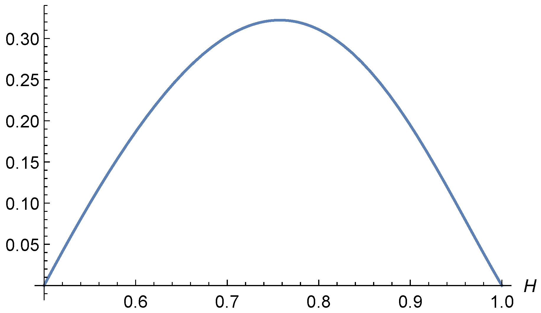
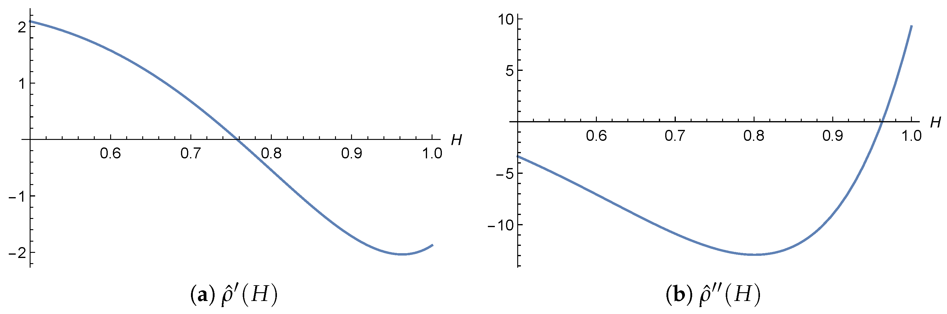
In particular, for the case n = 4 , we thoroughly investigated the coefficient Γ 4 3 of the one-sided projection and proved its positivity on a specific subinterval 1 2 , H 0 and in a neighborhood of 1. These findings complement the results of [18], where other coefficients of the one-sided projection for n = 4 were analyzed.
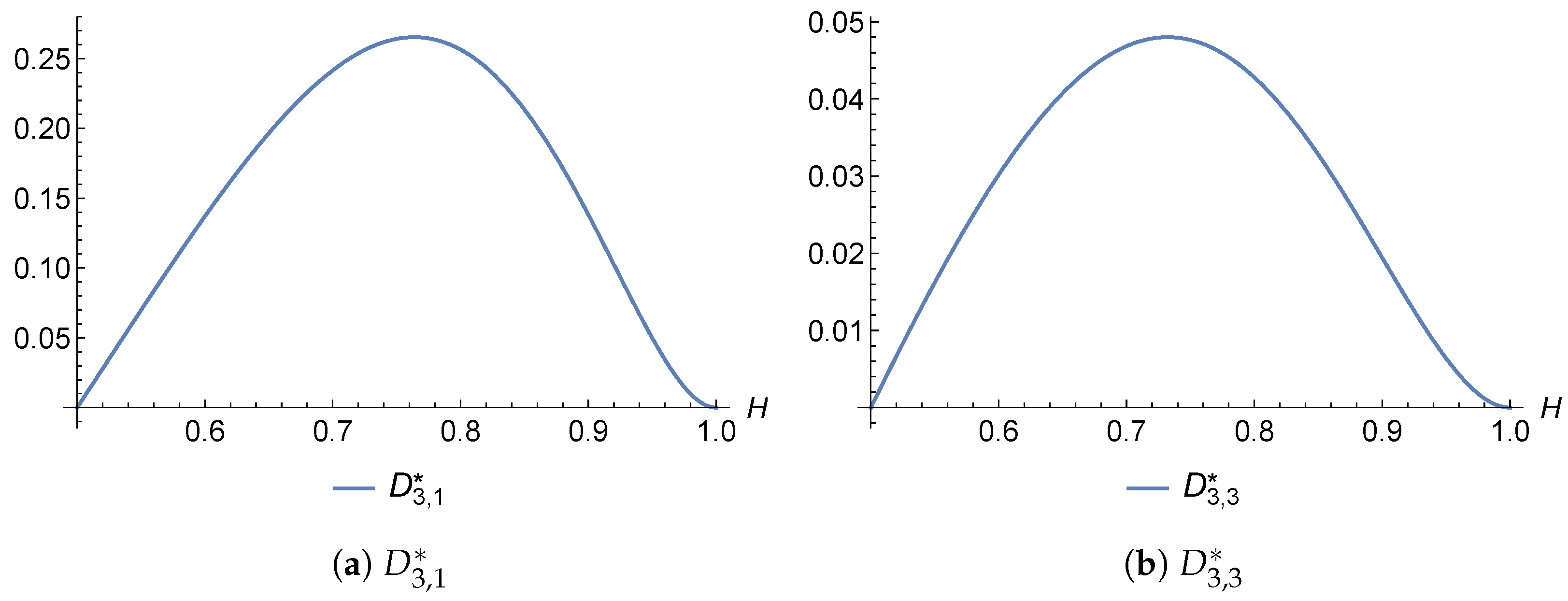
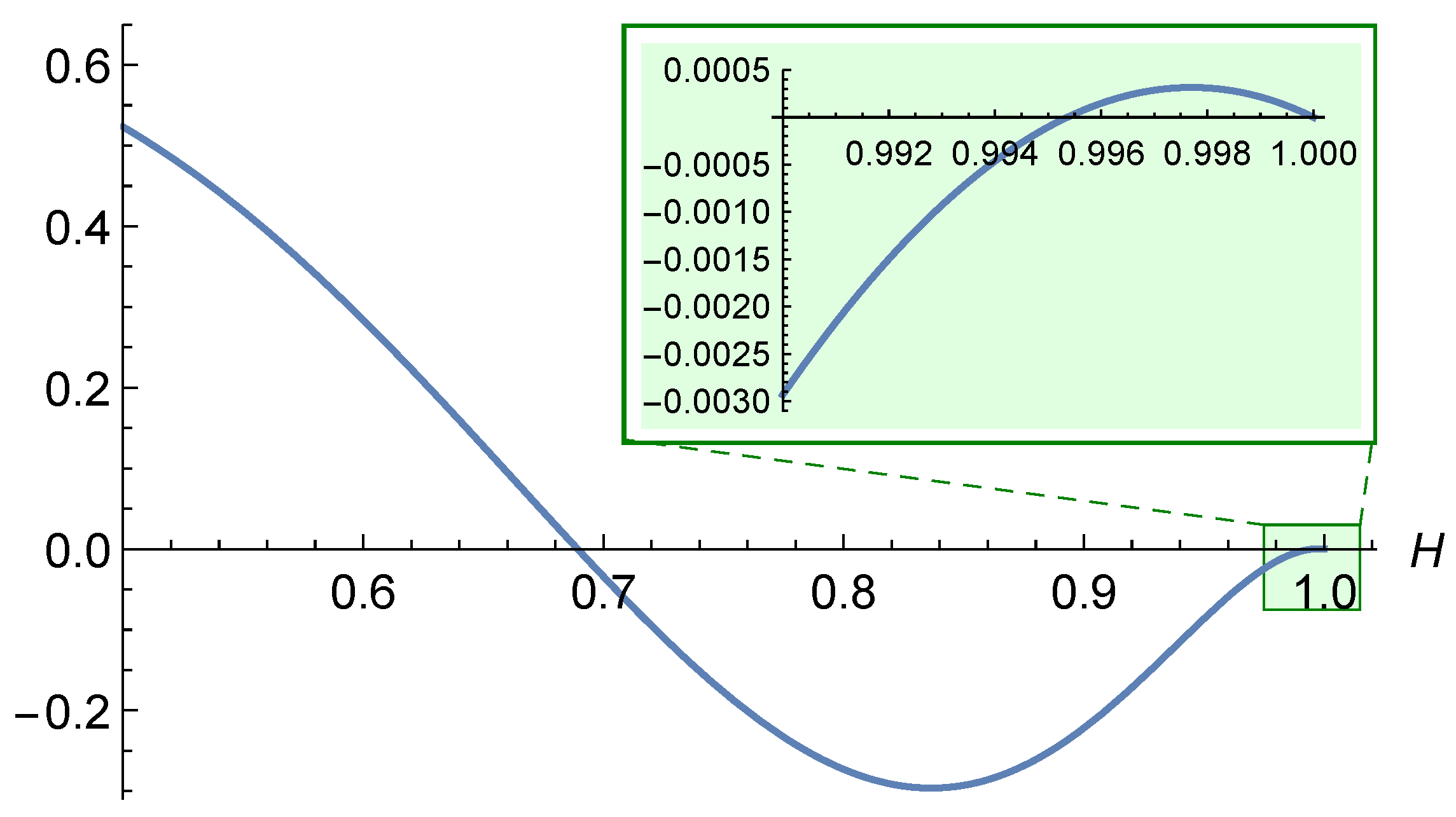
For the two-sided (bilateral) projection, we derived recurrence relations for the coefficients. These formulas are notably complex, especially for projections involving distant neighbors, and significant simplification appears unlikely. Therefore, we focused on specific cases with n = 2 , 3 , 4 , where the projection coefficient formulas are relatively tractable. For n = 2 and n = 3 , we obtained explicit expressions for the coefficients, established their strict positivity for all H ( 1 / 2 , 1 ) , and showed that they are concave functions of H. In the case n = 4 , a numerical analysis revealed that the coefficients Q 3 1 and Q 3 3 remain strictly positive for all H ( 1 / 2 , 1 ) . However, we also provided an analytical proof demonstrating that there exists some δ > 0 such that for any H ( δ , 1 ) , the coefficient Q 3 2 becomes negative.
Furthermore, we computed the coefficients Q n k numerically for various values of H and 1 n 10 , obtaining results consistent with the case n = 4 .
In addition, we analyzed the asymptotic behavior of the projection norm. Recurrence formulas for the norms of both one-sided and two-sided projections were derived, and their behavior was investigated numerically.
As a natural continuation of this work, it would be worthwhile to explore similar projection procedures applied to integrated fractional Brownian motion and the fractional Ornstein–Uhlenbeck process (see [25,26]). These processes are increasingly employed in applications as models of relatively smooth systems with memory.

Author Contributions

Investigation, I.B., Y.M., and K.R.; writing—original draft preparation, I.B., Y.M., and K.R. All authors have read and agreed to the published version of the manuscript.

Funding

Y.M. is supported by The Swedish Foundation for Strategic Research, grant UKR24-0004, and by the Japan Science and Technology Agency CREST, project reference number JPMJCR2115. K.R. is supported by the Research Council of Finland, decision number 367468. Y.M. and K.R. acknowledge that the present research is carried out within the frame of the ToppForsk project no. 274410 of the Research Council of Norway with the title STORM: Stochastics for time–space risk models.

Institutional Review Board Statement

Not applicable.

Data Availability Statement

No data was used for the research described in the article.

Conflicts of Interest

The authors declare no conflicts of interest.

References

  1. Beran, J. Statistics for Long-Memory Processes, 1st ed.; Monographs on Statistics and Applied Probability; Chapman & Hall: New York, NY, USA, 1994. [Google Scholar]
  2. Delignieres, D. Correlation properties of (discrete) fractional Gaussian noise and fractional Brownian motion. Math. Probl. Eng. 2015, 2015, 485623. [Google Scholar] [CrossRef]
  3. Liu, Y.; Liu, Y.; Wang, K.; Jiang, T.; Yang, L. Modified periodogram method for estimating the Hurst exponent of fractional Gaussian noise. Phys. Rev. E 2009, 80, 066207. [Google Scholar] [CrossRef] [PubMed]
  4. Mandelbrot, B.B.; Ness, J.W.V. Fractional Brownian motions, fractional noises and applications. SIAM Rev. 1968, 10, 422–437. [Google Scholar] [CrossRef]
  5. Mandelbrot, B.B. A fast fractional Gaussian noise generator. Water Resour. Res. 1971, 7, 543–553. [Google Scholar] [CrossRef]
  6. Meerson, B.; Bénichou, O.; Oshanin, G. Path integrals for fractional Brownian motion and fractional Gaussian noise. Phys. Rev. E 2022, 106, L062102. [Google Scholar] [CrossRef] [PubMed]
  7. Qian, H. Fractional Brownian motion and fractional Gaussian noise. In Processes with Long-Range Correlations: Theory and Applications; Springer: Berlin/Heidelberg, Germany, 2003; pp. 22–33. [Google Scholar]
  8. Wang, W.; Cherstvy, A.G.; Liu, X.; Metzler, R. Anomalous diffusion and nonergodicity for heterogeneous diffusion processes with fractional Gaussian noise. Phys. Rev. E 2020, 102, 012146. [Google Scholar] [CrossRef] [PubMed]
  9. Yamagishi, H.; Yoshida, N. Order estimate of functionals related to fractional Brownian motion. Stoch. Process. Appl. 2023, 161, 490–543. [Google Scholar] [CrossRef]
  10. Li, M.; Sun, X.; Xiao, X. Revisiting fractional Gaussian noise. Phys. A Stat. Mech. Its Appl. 2019, 514, 56–62. [Google Scholar] [CrossRef]
  11. Li, M. Modified multifractional Gaussian noise and its application. Phys. Scr. 2021, 96, 125002. [Google Scholar] [CrossRef]
  12. Molz, F.J.; Liu, H.H.; Szulga, J. Fractional Brownian motion and fractional Gaussian noise in subsurface hydrology: A review, presentation of fundamental properties, and extensions. Water Resour. Res. 1997, 33, 2273–2286. [Google Scholar] [CrossRef]
  13. Stratonovich, R.L. Theory of Information and Its Value; Belavkin, R.V., Pardalos, P.M., Principe, J.C., Eds.; Springer: Cham, Switzerland, 2020. [Google Scholar]
  14. Barton, R.J.; Poor, H.V. Signal detection in fractional Gaussian noise. IEEE Trans. Inf. Theory 1988, 34, 943–959. [Google Scholar] [CrossRef]
  15. D’avalos, A.; Jabloun, M.; Ravier, P.; Buttelli, O. Theoretical study of multiscale permutation entropy on finite-length fractional Gaussian noise. In Proceedings of the 2018 26th European Signal Processing Conference (EUSIPCO), Rome, Italy, 3–7 September 2018; pp. 1087–1091. [Google Scholar]
  16. Zunino, L.; Pérez, D.G.; Martín, M.T.; Garavaglia, M.; Plastino, A.; Rosso, O.A. Permutation entropy of fractional Brownian motion and fractional Gaussian noise. Phys. Lett. A 2008, 372, 4768–4774. [Google Scholar] [CrossRef]
  17. Bock, W.; Bornales, J.B.; Streit, L. Dynamical properties of Gaussian chains and loops with long-range interactions. Rep. Math. Phys. 2021, 88, 233–246. [Google Scholar] [CrossRef]
  18. Mishura, Y.; Ralchenko, K.; Schilling, R.L. Analytical and Computational Problems Related to Fractional Gaussian Noise. Fractal Fract. 2022, 6, 620. [Google Scholar] [CrossRef]
  19. Mishura, Y.; Ralchenko, K.; Shklyar, S. General conditions of weak convergence of discrete-time multiplicative scheme to asset price with memory. Risks 2020, 8, 11. [Google Scholar] [CrossRef]
  20. Bodnarchuk, I.; Mishura, Y. Combinatorial approach to the calculation of projection coefficients for the simplest Gaussian–Volterra process. Mod. Stochastics Theory Appl. 2024, 11, 403–419. [Google Scholar] [CrossRef]
  21. Gavassino, L. Life on a closed timelike curve. Class. Quantum Gravity 2024, 42, 015002. [Google Scholar] [CrossRef]
  22. Liptser, R.S.; Shiryaev, A.N. Statistics of Random Processes II: Applications, 2nd ed.; Springer: Berlin/Heidelberg, Germany, 2013. [Google Scholar]
  23. Mishura, Y.; Zili, M. Stochastic Analysis of Mixed Fractional Gaussian Processes; ISTE Press—Elsevier: London, UK, 2018. [Google Scholar]
  24. Banna, O.; Mishura, Y.; Ralchenko, K.; Shklyar, S. Fractional Brownian Motion. Approximations and Projections; Wiley-ISTE: London, UK, 2019. [Google Scholar]
  25. Abundo, M.; Pirozzi, E. Integrated stationary Ornstein-Uhlenbeck process, and double integral processes. Phys. A 2018, 494, 265–275. [Google Scholar] [CrossRef]
  26. Abundo, M.; Pirozzi, E. On the Integral of the Fractional Brownian Motion and Some Pseudo-Fractional Gaussian Processes. Mathematics 2019, 7, 991. [Google Scholar] [CrossRef]
Figure 1. Graph of ρ ^ ( H ) as a function of H.
Fractalfract 09 00428 g001
Figure 2. Graphs of derivatives ρ ^ ( H ) and ρ ^ ( H ) as functions of H.
Fractalfract 09 00428 g002
Figure 3. Graph of Q 1 1 as a function of H.
Fractalfract 09 00428 g003
Figure 4. Graphs of Q 2 1 and Q 2 2 as functions of H.
Fractalfract 09 00428 g004
Figure 5. Graphs of D 3 , 1 * and D 3 , 3 * as functions of H.
Fractalfract 09 00428 g005
Figure 6. Graph of D 3 , 2 * as a function of H.
Fractalfract 09 00428 g006
Figure 7. The derivative H D 3 , 2 * as a function of H.
Fractalfract 09 00428 g007
Figure 8. The second derivative H H D 3 , 2 * as a function of H.
Fractalfract 09 00428 g008
Figure 9. Graphs of Q 3 1 , Q 3 2 and Q 3 3 as functions of H.
Fractalfract 09 00428 g009
Figure 10. Graphs of Q 4 k , k = 1 , 2 , 3 , 4 , as functions of H.
Fractalfract 09 00428 g010
Figure 11. Graphs of Q 5 k , k = 1 , , 5 , as functions of H.
Fractalfract 09 00428 g011
Figure 12. Graphs of Q n 2 , n = 2 , , 6 , as functions of H. Points of intersection with H axis.
Fractalfract 09 00428 g012
Figure 13. Norms R 1 ( n ) (left) and R 2 ( n ) (right) as functions of n for H = 0.6 , 0.7 , 0.8 , 0.9 .
Fractalfract 09 00428 g013aFractalfract 09 00428 g013b
Figure 14. Norms R 1 ( n ) and R 2 ( n ) for n = 500 .
Fractalfract 09 00428 g014
Table 1. Coefficients Q n k for H = 0.51 .
n k 12345678910
10.013884
20.0137950.005149
30.0137690.0050960.003342
40.0137560.0050790.0033040.002480
50.0137470.0050700.0032920.0024510.001973
60.0137420.0050640.0032840.0024410.0019490.001638
70.0137380.0050590.0032790.0024350.0019400.0016170.001400
80.0137350.0050560.0032760.0024310.0019350.0016100.0013830.001223
90.0137320.0050540.0032730.0024280.0019320.0016060.0013760.0012070.001085
100.0137300.0050520.0032710.0024250.0019290.0016030.0013720.0012020.0010710.000975
Table 2. Coefficients Q n k for H = 0.6 .
n k 12345678910
10.138815
20.1307390.043422
30.1286480.0388620.028344
40.1275920.0376390.0251920.020583
50.1269650.0369690.0243140.0181840.016087
60.1265520.0365490.0238140.0175030.0141580.013157
70.1262600.0362610.0234900.0171040.0136030.0115480.011103
80.1260440.0360510.0232620.0168410.0132720.0110810.0097250.009585
90.1258780.0358920.0230920.0166530.0130510.0107990.0093220.0083820.008419
100.1257460.0357670.0229620.0165110.0128910.0106090.0090770.0080290.0073540.007498
Table 3. Coefficients Q n k for H = 0.7 .
n k 12345678910
10.268776
20.2422780.067642
30.2361010.0528120.045780
40.2330650.0496610.0359270.032171
50.2313460.0479320.0337500.0248520.024639
60.2302550.0468970.0324930.0232120.0188680.019801
70.2295090.0462100.0317150.0222340.0175610.0150650.016460
80.2289710.0457250.0311840.0216150.0167650.0139850.0124630.014025
90.2285670.0453650.0308000.0211850.0162540.0133170.0115460.0105790.012178
100.2282550.0450890.0305100.0208690.0158940.0128830.0109730.0097850.0091580.010733
Table 4. Coefficients Q n k for H = 0.8 .
n k 12345678910
10.376892
20.3327550.073057
30.3232180.0467630.053946
40.3186430.0426410.0373400.036154
50.3161900.0402740.0345830.0240790.027185
60.3146890.0389390.0328950.0220660.0178490.021453
70.3136950.0380830.0319080.0207800.0162830.0139150.017566
80.3129990.0374950.0312550.0200110.0152540.0126460.0112910.014771
90.3124890.0370710.0307960.0194920.0146280.0117940.0102320.0094280.012677
100.3121030.0367530.0304570.0191210.0142000.0112710.0095100.0085240.0080450.011056
Table 5. Coefficients Q n k for H = 0.9 .
n k 12345678910
10.454626
20.4039220.062598
30.3931750.0266120.055279
40.3881170.0229140.0341590.034475
50.3855600.0204880.0317500.0193330.025609
60.3840530.0192290.0300420.0176460.0141440.019817
70.3830880.0184450.0291200.0163700.0128690.0107060.015985
80.3824300.0179240.0285260.0156660.0118620.0096970.0085070.013264
90.3819610.0175570.0281200.0152020.0112980.0088750.0076820.0069730.011252
100.3816130.0172890.0278280.0148790.0109210.0084090.0069920.0062810.0058570.009711
Table 6. Coefficients Q n k for H = 0.99 .
n k 12345678910
10.496847
20.4545610.043067
30.4447150.0009380.052726
40.440112 0.001495 0.0303790.029737
50.437912 0.003621 0.0288330.0137180.022123
60.436656 0.004607 0.0273500.0127020.0102570.016765
70.435877 0.005212 0.0266300.0116100.0095200.0074630.013351
80.435359 0.005601 0.0261730.0110710.0086690.0069000.0058130.010945
90.434998 0.005868 0.0258690.0107190.0082430.0062120.0053660.0046730.009187
100.434735 0.006059 0.0256560.0104820.0079610.0058650.0047940.0043070.0038620.007854
Table 7. Norms R 1 ( n ) and R 2 ( n ) for various n.
n250100200300400
H = 0.6 R 1 ( n ) 0.0221110.0282810.0283800.0284290.0284450.028453
R 2 ( n ) 0.0412830.0497370.0498130.0498460.0498560.049860
H = 0.7 R 1 ( n ) 0.1020850.1240710.1244270.1246040.1246620.124692
R 2 ( n ) 0.1717520.1903550.1904510.1904870.1904960.190500
H = 0.8 R 1 ( n ) 0.2659640.3054130.3060500.3063650.3064690.306521
R 2 ( n ) 0.3887390.4070760.4071310.4071490.4071540.407155
H = 0.9 R 1 ( n ) 0.5492310.5914060.5920720.5924020.5925110.592565
R 2 ( n ) 0.6738470.6832180.6832350.683240.6832410.683242
H = 0.99 R 1 ( n ) 0.9456890.9531880.9533020.9533590.9533780.953387
R 2 ( n ) 0.9663340.9670780.9670790.9670790.9670790.967079
Disclaimer/Publisher’s Note: The statements, opinions and data contained in all publications are solely those of the individual author(s) and contributor(s) and not of MDPI and/or the editor(s). MDPI and/or the editor(s) disclaim responsibility for any injury to people or property resulting from any ideas, methods, instructions or products referred to in the content.

