Solvability of Fuzzy Partially Differentiable Models for Caputo–Hadamard-Type Goursat Problems Involving Generalized Hukuhara Difference

Abstract

In this paper, we investigate a class of fuzzy partially differentiable models for Caputo–Hadamard-type Goursat problems with generalized Hukuhara difference, which have been widely recognized as having a significant role in simulating and analyzing various kinds of processes in engineering and physical sciences. By transforming the fuzzy partially differentiable models into equivalent integral equations and employing classical Banach and Schauder fixed-point theorems, we establish the existence and uniqueness of solutions for the fuzzy partially differentiable models. Furthermore, in order to overcome the complexity of obtaining exact solutions of systems involving Caputo–Hadamard fractional derivatives, we explore numerical approximations based on trapezoidal and Simpson’s rules and propose three numerical examples to visually illustrate the main results presented in this paper.

1. Introduction

In the 17th century, integral and differential equations emerged as powerful mathematical tools. Over nearly four centuries of development, researchers have conducted increasingly in-depth investigations into these calculus-based equations. Emerging as a product of the development of differential equations, the following Goursat problem, which plays an important role in describing wave phenomena such as sound and light waves [1], is a classic hyperbolic partial differential equation model:

$${\zeta }_{xy}=f(x,y,\zeta ,{\zeta }_x,{\zeta }_y),\forall (x,y)\in P,$$

(1)

where $\zeta$ is a real-valued function defined on a rectangular domain (P) around the origin in ${\mathbb{R}}^2$; ${\zeta }_{x,y}$ denotes the mixed partial derivative of $\zeta$ with respect to x and y; and ${\zeta }_x$ and ${\zeta }_y$ are partial derivatives of $\zeta$ with respect to x and y, respectively. These derivatives are assumed to exist and be continuous. Additionally, the function expressed as $f(x,y,\zeta ,{\zeta }_x,{\zeta }_y)$ is bounded and continuous on $P\times {\mathbb{R}}^3$.

It is well known that the fuzzy set theory proposed by Zadeh [2] has attracted widespread research attention. Various extensions, including intuitionistic, hesitant, and Pythagorean fuzzy sets, have been developed, contributing to the growing maturity of fuzzy set theory. In contrast to the partial differential equations formulated on classical sets by Bers et al. [3] in 1964, Buckley et al. [4] introduced fuzzy partial differential equations to offer a more comprehensive and detailed representation of uncertain information systems. Fuzzy partial differential equations also represent a new direction in the development of traditional partial differential equation models, including models of the form of Equation (1).

On the other hand, to meet the requirements of various environments, different types of fractional derivatives have been developed to describe the dynamics of diverse systems. As a result, fractional-order differential equations (FDEs) have gained prominence for their suitability in addressing specific problems compared to their integer-order counterparts. As highlighted in previous studies, fractional calculus is characterized by time-memory effects and long-range spatial correlations, which allow for more accurate modeling of physical and biochemical processes exhibiting memory, inheritance, and path dependence. Consequently, FDEs have become an essential component of both mathematical theory and applied investigation. Moreover, they offer valuable insights to researchers across a wide range of disciplines. Their applicability has led to successful implementations in fields such as biotechnology [5], physics [6], and material mechanics [7].

Compared with other types of fractional calculus (e.g., Caputo and Riemann–Liouville calculus), Hadamard-type fractional calculus, which was initially introduced in 1892 by Hadamard [8], received relatively little attention from researchers in its early stages. Notably, unlike the Caputo and Riemann–Liouville derivatives, the integral kernel of the Hadamard-type derivative is a logarithmic function in the form of $\left(\log \left(x\right)-\log \left(s\right)\right)$ rather than $\left(x-s\right)$. Moreover, the Hadamard derivative can be regarded as a generalization of the operator expressed as ${\left(x{\displaystyle \frac{d}{dx}}\right)}^n$. Due to these characteristics, the Hadamard-type derivative is particularly well-suited for modeling phenomena on the half-axis [9]. In recent decades, these distinctive properties have attracted increasing interest in Hadamard-type fractional differential equations. In 2001, Kilbas [10] investigated Hadamard-type fractional calculus on a finite real interval $[a,b]$, and in 2003, Kilbas [11] further addressed the following Hadamard-type integral equation:

$${\displaystyle \frac{1}{\Gamma \left(\alpha \right)}}{\int }_a^x{\left({\displaystyle \frac{z}{x}}\right)}^{\mu }{\left(\log \left({\displaystyle \frac{x}{z}}\right)\right)}^{\alpha -1}f\left(z\right){\displaystyle \frac{dz}{z}}=g\left(x\right),$$

where $\alpha >0$, $\mu$ is a real number and f is a Lebesgue integrable function defined on the interval of $(a,b)$. Salem [12] introduced several definitions and properties of Hadamard-type fractional operators in Banach spaces. In recent years, research on Hadamard-type fractional differential equations has continued to deepen. For instance, Li et al. [13] proposed a definition of the fractional Lyapunov exponent for Hadamard-type fractional differential systems, and Zhang et al. [14] studied the existence of solutions to a class of Hadamard-type problems. Similarly, several other types of fractional derivatives, such as the Grunwald–Letnikov [15] and Caputo–Hadamard types [16], have emerged alongside the rapid development of FDEs. We notice that the majority of researchers focus on extensions of Caputo-type and Riemann–Liouville-type derivatives. The Caputo–Hadamard fractional derivative integrates the features of both Caputo and Hadamard fractional derivatives, in the sense that its integral kernel is of logarithmic type, specifically of the form $\left(\log \left(x\right)-\log \left(s\right)\right)$, and contains an nth-order differential operator (${\left(x{\displaystyle \frac{d}{dx}}\right)}^n$). This modification of the integral kernel represents a broader approach to capturing the dynamics of complex systems and expands the applicability and utility of fractional calculus across various scientific domains. Subsequently, Gohar et al. [17] determined the existence and uniqueness of solutions for the following Caputo–Hadamard fractional differential system in a crisp environment:

$$\left\{\begin{array}{c}{}_{CH}D_{a^{+}}^{\alpha }u\left(t\right)=f(t,u),t>a^{+}>0,0<\alpha <1,\hfill \\ u\left(a^{+}\right)=u_a,\hfill \end{array}\right.$$

where ${}_{CH}D_{a^{+}}^{\alpha }u$ is an $\alpha$-order Caputo–Hadamard-type derivative for a given function (u); f is a continuous function; and $u_a$ is the initial value, which is equivalent to the Volterra integral equation:

$$u\left(t\right)=u_a+{\displaystyle \frac{1}{\Gamma \left(\alpha \right)}}{\int }_a^t{\left(\log \left({\displaystyle \frac{t}{s}}\right)\right)}^{\alpha -1}f(s,u\left(s\right)){\displaystyle \frac{ds}{s}}.$$

However, as the study of FDEs has advanced, some researchers have observed that conventional FDEs often fail to adequately characterize complex systems involving fuzzy information [18]. To overcome these limitations, fuzzy fractional-order differential equations (FFDEs) have been proposed as a promising alternative. The integration of fuzzy information into FDEs was first proposed in 1989, marking the beginning of sustained research interest in this field. A major development in FFDEs is the introduction of the fuzzy Laplace transform [19], which offers a more efficient method for solving FFDEs with Riemann–Liouville Hukuhara (H-) differentiability. Furthermore, based on both analytical and approximate consistent solutions, Arqub et al. [20] demonstrated the applicability of a generalized fuzzy conformable FDE, expressed as follows:

$$D^{\beta }u\left(t\right)=\underset{\epsilon \to 0^{+}}{lim}{\displaystyle \frac{u\left(t\right)\ominus u{(t+\epsilon (t-t_0))}^{1-\beta }}{-\epsilon }},$$

where $\beta \in (0,1]$ denotes the order of the fuzzy conformable fractional derivative ($D^{\beta }u$) and ⊖ represents the H difference.

It is well known that for numerical solutions of fuzzy linear systems, the tau method in combination with Jacobi polynomials exhibits strong applicability, improving both robustness and accuracy in result simplification [21]. Meanwhile, various numerical integration methods [22], such as the trapezoidal rule [23], Simpson’s rule [23], and the Gaussian quadrature rule [22], may provide valuable tools for obtaining approximate solutions to FFDEs. To better accommodate fuzzy environments, researchers have proposed various innovative theories and methods for FFDEs. These include the fuzzy Laplace and Fourier transforms [24], Pythagorean fuzzy partial differential equation models [24], and the Adomian decomposition method [25]. More detailed information about the above works can be found in [26] and the references therein.

Moreover, Aliev et al. [27] developed the H-difference form of Z numbers, and Amma et al. [28] demonstrated the existence and uniqueness of solutions for a class of intuitionistic fuzzy-set fractional partial differential equations (FFPDEs). The fact that traditional H difference is often criticized for its limitations can be ignored. Unlike the classical H difference, the operational criteria and properties of the interval-valued function space, which were constructed based on the generalized Hukuhara (gH-)-type difference (${\ominus }_{gH}$), can be applied to the following semi-linear interval differential equations [29]:

$$\begin{array}{c}(f+g)\left(t\right)=f\left(t\right)+g\left(t\right),\hfill \\ \left(kf\right)\left(t\right)=kf\left(t\right),\forall k\in \mathbb{R},\hfill \\ \left(f{\ominus }_{gH}g\right)\left(t\right)=f\left(t\right){\ominus }_{gH}g\left(t\right),\hfill \\ \left(fg\right)\left(t\right)=f\left(t\right)g\left(t\right).\hfill \end{array}$$

The application of suitable forms of gH-fractional derivatives in FFPDEs is also prevalent (see [30]). These advancements have substantially enriched the toolbox for modeling and solving complex dynamic systems. In particular, Zhang et al. [31] studied the two gH-type weak solutions for the following Caputo fractional derivative coupled system in a fuzzy gH-difference environment:

$$\left\{\begin{array}{l}{}_{gH}{}^{C }D_k^{\alpha }u(x,y)=f(x,y,v(x,y)),\\ {}_{gH}{}^{C }D_k^{\beta }v(x,y)=g(x,y,u(x,y))\end{array}\right.$$

with initial condition of

$$\left\{\begin{array}{ll}u(x,0)={\xi }_1\left(x\right),v(x,0)={\eta }_1\left(x\right),\hfill & \hfill \forall x\in [0,a],\\ u(0,y)={\xi }_2\left(y\right),v(0,y)={\eta }_2\left(y\right),\hfill & \hfill \forall y\in [0,b],\end{array}\right.$$

where $k=1,2$, $\alpha =({\alpha }_1,{\alpha }_2),\beta =({\beta }_1,{\beta }_2)\in (0,1]\times (0,1]$ are fractional orders of Caputo gH-type derivative operators ${}_{gH}{}^{C }D_k^{\alpha }$ and ${}_{gH}{}^{C }D_k^{\beta }$, respectively.

Inspired by the works reported in [17,31], in combination with the results of [1], we consider the following fuzzy Goursat problem involving a Caputo–Hadamard-type fractional derivative with gH difference:

$$\left\{\begin{array}{l}{}_{CH}{}^{\theta }D_{xy}^{i,l}u(x,y)=a_1{}_{CH}{}^{\theta }D_x^{i}u(x,y)+a_2{}_{CH}{}^{\theta }D_y^{l}u(x,y)+a_{3}u(x,y)+a_{4}G(x,y),\hfill \\ u(x,y_0)={\varphi }_1\left(x\right),x_0\le x\le T,\hfill \\ u(x_0,y)={\varphi }_2\left(y\right),y_0\le y\le T,\hfill \end{array}\right.$$

(2)

where constant $a_{\iota }$ pertains to the domain of $\mathbb{R}$ for any $\iota =1,2,3,4$ and $G:\mathbf{X}\to \mathbb{R}$ is a continuously differentiable function in the closed region of $\mathbf{X}=[x_0,T]\times [y_0,T]$. Initial value functions ${\varphi }_1\left(x\right):[x_0,T]\to \mathbb{E}$ and ${\varphi }_2\left(y\right):[y_0,T]\to \mathbb{E}$ are also continuously bounded, and ${\varphi }_1\left(0\right)={\varphi }_2\left(0\right)$. For all orders ($\theta \in (0,1]$) of fractional partial differential derivatives, each $i,l\in \{1,2\}$, and any $u\in C_{i,l}(\mathbf{X},\mathbb{E})$, the space of continuous functions from $\mathbf{X}$ to $\mathbb{E}$, ${}_{CH}{}^{\theta }D_{xy}^{i,l}u$ is Caputo–Hadamard gH-type mixed partial differential operator shown later in Remark 4, and ${}_{CH}{}^{\theta }D_x^i$ and ${}_{CH}{}^{\theta }D_y^l$, as defined in Definition 7, separately represent Caputo–Hadamard gH-type partial differential operators in regard to variables x and y. Here, different values of i and l correspond to distinct spaces and the type († or ‡) of partial differentiability with respect to x and y, respectively (for instance, ${}_{CH}{}^{\theta }D_x^{1}u$ and ${}_{CH}{}^{\theta }D_x^{2}u$ imply that u is †-type and ‡-type partially differentiable with respect to x).

Remark 1.

(i) If the order is $\theta =1$, then (1) will be degenerated to the form of integer order. Thus, we extend (1) to (2) by generalizing the classical integer-order Goursat problem to a Goursat problem with a Caputo–Hadamard fractional order derivative; here, the integral kernel takes the form of a logarithmic function. This extension provides a feasible direction for future research on the chaotic dynamical behavior of the equation model (2), as well as circuit design and communication applications.

(ii) To accommodate Caputo–Hadamard-type derivatives in the Goursat problem, we shall refine the metric fixed-point method employed in [1].

(iii) Additionally, we introduce a fuzzy environment (i.e., gH difference) to enhance the comprehensiveness of real-world problems that can be modeled by the system (2).

The rest of this paper is organized as follows: In Section 2, we review several fundamental properties and establish some useful results in this study. By employing Banach and Schauder fixed-point theorems, the existence and uniqueness of solutions for (2) are provided in Section 3. Using trapezoidal and Simpson’s rules [23], we illustrate the numerical approximation form of the solutions of (2) via two examples in Section 4. Finally, the work conducted in this paper is summarized and potential directions for future research are proposed in Section 5.

2. Preliminaries

In this section, in order to better handle (2), we first recall some concepts and properties from previous work on fuzzy fractional-order Caputo–Hadmard-type derivatives.

Throughout this paper, let $\Xi$ represent classical fuzzy sets in fuzzy environments. Then, $\Xi$ is fuzzy convex, upper semi-continuous, and compactly supported and represents a fuzzy number space. All spaces composed of $\Xi$ are called fuzzy spaces, as represented by $\mathbb{E}$. In the same way, for membership function L, the following conditions are met:

(i) L is upper semicontinuous.

(ii) $L(\lambda x_1+(1-\lambda )x_2)\ge min\{L\left(x_1\right)$, $L\left(x_2\right)\}$ for each $x_1,x_2\in \mathbb{R}$ and any $\lambda \in [0,1]$.

(iii) There exists $x_0\in \mathbb{R}$ such that $L\left(x_0\right)=1$.

(iv) $\mathrm{supp}L=cl\{x\in \mathbb{R}:L(x)>0\}$ is compact, where $cl$ represents closure of the set.

Definition 1.

([32]) The highest measure ($d_{\mathbb{E}}$) defined on $\mathbb{E}$ is expressed as

$$\begin{array}{cc}\hfill d_{\mathbb{E}}(p,q)& =\underset{r\in [0,1]}{sup}{d}_H\left({\left[p\right]}^r,{\left[q\right]}^r\right)\hfill \\ \hfill & =\underset{r\in [0,1]}{sup}max\left\{|{\underline{p}}_r-{\underline{q}}_r|,|{\overline{p}}_r-{\overline{q}}_r|\right\},\forall p,q\in \mathbb{E},\hfill \end{array}$$

(3)

where ${\left[p\right]}^r$ represents the r-level set of fuzzy number p (the r-level set of q is also represented similarly), as determined by

$${\left[p\right]}^r=\left\{\begin{array}{l}\{x\in \mathbb{R}:p(x)\ge r\}, for0<r\le 1,\\ cl\left(\mathrm{supp}p\right),forr=0,\hfill \end{array}\right.$$

where ${\underline{p}}_r$ represents the left endpoint and ${\overline{p}}_r$ represents the right endpoint of p.

In the sequel, let $len{\left[p\right]}^r={\overline{p}}_r-{\underline{p}}_r$ be the diameter of the r-level set of p and $h(x;r)$ denote the r-level set of the $h\left(x\right)$ function for all $x\in \mathbb{R}$.

Lemma 1.

([33]) If the measure space $(\mathbb{E},d_{\mathbb{E}})$ satisfying the elimination rule ($a+b=a+c\Rightarrow b=c$) for each $a,b,c\in (\mathbb{E},d_{\mathbb{E}})$ is complete and semilinear, then for any $\varpi \in (\mathbb{E},d_{\mathbb{E}})$,

$\left(m_1\right)$ $d_{\mathbb{E}}(a+b,c+\varpi )\le d_{\mathbb{E}}(a,c)+d_{\mathbb{E}}(b,\varpi )$;

$\left(m_2\right)$ If $a\ominus b,c\ominus \varpi$ exist, then $d_{\mathbb{E}}(a\ominus b,c\ominus \varpi )\le d_{\mathbb{E}}(a,c)+d_{\mathbb{E}}(b,\varpi )$;

$\left(m_3\right)$ $a\ominus (b+c)=a\ominus b\ominus c$ when $a\ominus (b+c)$ and $a\ominus b\ominus c$ exist;

$\left(m_4\right)$ If $a\ominus (b\ominus c)$ and $a\ominus b$ both exist, $a\ominus (b\ominus c)=a\ominus b+c$;

$\left(m_5\right)$ $(-1)(a\ominus b)=(-1)a\ominus (-1)b$ is valid if $a\ominus b$ and $(-1)a\ominus (-1)b$ exist.

Here, ⊖ represents the H difference, which is defined as follows:

$${\left[a\ominus b\right]}^r=\left[{\underline{a}}_r-{\underline{b}}_r,{\overline{a}}_r-{\underline{b}}_r\right]$$

Definition 2.

([34]) Letting $p_1,p_2,p_3\in \mathbb{E}$, the gH difference is defined as

$$p_1{\ominus }_{gH}{p}_2=p_3⟺\left\{\begin{array}{c}(†)p_1=p_2+p_3,\hfill \\ or(‡)p_2=p_1+(-1)p_3.\hfill \end{array}\right.$$

Remark 2.

([35]) According to Definition 2, the r-level set of $p_1{\ominus }_{gH}{p}_2$ can be represented as ${\left[p_1{\ominus }_{gH}{p}_2\right]}^r=\left[\underline{{\rm Y}},\overline{{\rm Y}}\right]$ for $p_1,p_2\in \mathbb{E}$, where $\underline{{\rm Y}}=min\left\{\underline{p_1}\left(r\right)-\underline{p_2}\left(r\right),\overline{p_1}\left(r\right)-\overline{p_2}\left(r\right)\right\}$ and $\overline{{\rm Y}}=max\{\underline{p_1}\left(r\right)-\underline{p_2}\left(r\right),$$\overline{p_1}\left(r\right)-\overline{p_2}\left(r\right)\}$.

Lemma 2.

([36]) Let $h\left(x\right)$ be a fuzzy set-valued function defined on $[x_1,\infty ]$ and characterized by its representation in terms of $\left(\underline{h}(x;r),\overline{h}(x;r)\right)$. Here, $\underline{h}(x;r)$ and $\overline{h}(x;r)$ denote the left and right endpoint functions corresponding to the level-set parameter (r), respectively. For any $r\in [0,1]$, both $\underline{h}(x;r)$ and $\overline{h}(x;r)$ are Riemann-integrable.

In addition, for any $x\in [x_0,x_1]$, integrals ${\int }_{x_0}^{x_1}\left|\underline{h}(x;r)\right|dx$ and ${\int }_{x_0}^{x_1}\left|\overline{h}(x;r)\right|dx$ are bounded by $\underline{K}\left(r\right)$ and $\overline{K}\left(r\right)$, respectively, that is,

$${\int }_{x_0}^{x_1}\left|\underline{h}(x;r)\right|dx\le \underline{K}\left(r\right),{\int }_{x_0}^{x_1}\left|\overline{h}(x;r)\right|dx\le \overline{K}\left(r\right).$$

Therefore, $h\left(x\right)$ is referred to as an abnormal fuzzy Riemann-integrable function on $[x_1,\infty ]$, and its integral is also a fuzzy number given by

$${\int }_{x_0}^{\infty }h(x;r)dx=\left[{\int }_{x_0}^{\infty }\underline{h}(x;r)dx,{\int }_{x_0}^{\infty }\overline{h}(x;r)dx\right].$$

Definition 3.

([1]) For point $(x_0,y_0)\in (x_1,x_2)\times (y_1,y_2)\subset P$, P is the same as in (1), and $g:(x_1,x_2)\times (y_1,y_2)\to \mathbb{E}$ is said to be first-order generalized fuzzy partial differentiable to x, if the following relationship with respect to $g(x_0,y_0)$ exists:

(i)

$$\underset{\varrho \to 0}{lim}{\displaystyle \frac{g(x_0+\varrho ,y_0){\ominus }_{gH}g(x_0,y_0)}{\varrho }}=\underset{\varrho \to 0}{lim}{\displaystyle \frac{g(x_0,y_0){\ominus }_{gH}g(x_0-\varrho ,y_0)}{\varrho }}=g_x^{\prime }(x_0,y_0)$$

for a small enough given number ($\varrho >0$) and gH differences of both $g(x_0+\varrho ,y_0){\ominus }_{gH}g(x_0,y_0)$ and $g(x_0,y_0){\ominus }_{gH}g(x_0-\varrho ,y_0)$ existing in $(\mathbb{E},d_{\mathbb{E}})$.

(ii) Given a small enough number ($\hslash >0$), if gH differences of both $g(x_0,y_0){\ominus }_{gH}g(x_0+\hslash ,y_0)$ and $g(x_0-\hslash ,y_0){\ominus }_{gH}g(x_0,y_0)$ exist in $(\mathbb{E},d_{\mathbb{E}})$, then one has

$$\underset{\hslash \to 0}{lim}{\displaystyle \frac{g(x_0,y_0){\ominus }_{gH}g(x_0+\hslash ,y_0)}{-\hslash }}=\underset{\hslash \to 0}{lim}{\displaystyle \frac{g(x_0-\hslash ,y_0){\ominus }_{gH}g(x_0,y_0)}{-\hslash }}=g_x^{\prime }(x_0,y_0).$$

We call the case (i) †-type partial differentiable and case (ii) ‡-type partially differentiable. Similar definitions can also be extended to †- and ‡-type partial derivatives with respect to y, as well as to higher-order generalized fuzzy partial derivatives.

Remark 3.

([35]) For $g:(x_1,x_2)\times (y_1,y_2)\to \mathbb{E}$ and the level-set parameter (r), suppose that there exists $(x_0,y_0)\in$$(x_1,x_2)\times (y_1,y_2)$ such that $\overline{g}(·,·;r)$ and $\underline{g}(·,·;r)$ are both partially differentiable at $(x_0,y_0)$. Then,

(i) The following relationship holds if g is †-type partially differentiable:

$$g_x^{\prime }(x,y)(x_0,y_0;r)=\left[\left({\underline{g}}_x^{\prime }\right)(x_0,y_0;r),\left({\overline{g}}_x^{\prime }\right)(x_0,y_0;r)\right];$$

(ii) The following correlation holds when g is ‡-type partially differentiable.

$$g_x^{\prime }(x,y)(x_0,y_0;r)=\left[\left({\overline{g}}_x^{\prime }\right)(x_0,y_0;r),\left({\underline{g}}_x^{\prime }\right)(x_0,y_0;r)\right].$$

For the partial derivative of g with respect to y, similar results are also applicable, which are not presented here.

Lemma 3.

([37]) (Schauder fixed-point theorem) Λ is a bounded, closed, convex set that exists in a Banach space, and assuming that there is a self-mapping (S) that is completely continuous, we say that the mapping (S) has a fixed point in Λ.

Lemma 4.

([37]) (Banach fixed-point theorem) If Ω is a complete metric space (i.e., every Cauchy sequence in Ω converges to a point within Ω) and f is a contraction mapping on Ω, then f has a unique fixed point ($x^{\ast }\in \Omega$) such that $f\left(x^{\ast }\right)=x^{\ast }$.

Here, a contraction mapping refers to a function ($f:\Omega \to \Omega$) such that there exists a constant ($0\le \tau <1$) for which the following inequality holds for all $u,v\in \Omega$:

$$d\left(f\left(u\right),f\left(v\right)\right)\le \tau ·d(u,v),$$

where d denotes the metric on Ω.

Definition 4.

([38]) Under the condition of order $\theta >0$, the Hadamard gH-type fractional integral for the given function (f) is the fuzzy value function above $f\in {\mathcal{C}}^F[a,b]\cap {\mathcal{L}}^F[a,b]$ (f is a real-valued function defined on the interval of $[a,b]$ that is both fuzzy continuous and fuzzy Lebesgue-integrable) and is defined as follows: for each $x>a>0$,

$${}^{H}I_a^{\theta }f\left(x\right)={\displaystyle \frac{1}{\Gamma \left(\theta \right)}}{\int }_a^x{\left(\log {\displaystyle \frac{x}{s}}\right)}^{\theta -1}f\left(s\right){\displaystyle \frac{ds}{s}},$$

and the following results apply to the r-level sets associated with the Hadamard gH-type integral:

(i) If f is †-type differentiable, it is evident that the associated r-level set satisfies the following relationship:

$${{[}^H{I}_a^{\theta }f\left(x\right)]}^r=\left[{\displaystyle \frac{1}{\Gamma \left(\theta \right)}}{\int }_a^x{\left(\log {\displaystyle \frac{x}{s}}\right)}^{\theta -1}\underline{f}(s;r){\displaystyle \frac{ds}{s}},{\displaystyle \frac{1}{\Gamma \left(\theta \right)}}{\int }_a^x{\left(\log {\displaystyle \frac{x}{s}}\right)}^{\theta -1}\overline{f}(s;r){\displaystyle \frac{ds}{s}}\right].$$

(ii) Otherwise, it is clear to see that the related r-level set fulfills

$${{[}^H{I}_a^{\theta }f\left(x\right)]}^r=\left[{\displaystyle \frac{1}{\Gamma \left(\theta \right)}}{\int }_a^x{\left(\log {\displaystyle \frac{x}{s}}\right)}^{\theta -1}\overline{f}(s;r){\displaystyle \frac{ds}{s}},{\displaystyle \frac{1}{\Gamma \left(\theta \right)}}{\int }_a^x{\left(\log {\displaystyle \frac{x}{s}}\right)}^{\theta -1}\underline{f}(s;r){\displaystyle \frac{ds}{s}}\right],$$

when $f\left(x\right)$ is ‡-type differentiable.

Definition 5.

([38]) For all $x>a>0$, the Hadamard gH-type fractional derivative for a given function (f) is a fuzzy value function on ${\mathcal{C}}^F[a,b]\cap {\mathcal{L}}^F[a,b]$ and is defined as

$${}^{H}D^{\theta }f\left(x\right)={\displaystyle \frac{1}{\Gamma (n-\theta )}}{\delta }^n{\int }_a^x{\left(\log {\displaystyle \frac{x}{s}}\right)}^{n-\theta -1}f\left(s\right){\displaystyle \frac{ds}{s}},$$

and the fractional order is $\theta \in (n-1,n)$, where $n\in {\mathbb{Z}}^{+}$ and ${\delta }^n={\left(x{\displaystyle \frac{d}{dx}}\right)}^n$ is the n-order derivative of Hadamard-type differentiation ($x{\displaystyle \frac{d}{dx}}$).

Definition 6.

([39]) Under the condition of order $\theta >0$, the Caputo–Hadamard gH-type fractional derivative for a given function (f) on ${\mathcal{C}}^F[a,b]\cap {\mathcal{L}}^F[a,b]$ is defined as

$${}^{CH}D_a^{\theta }f\left(x\right)={\displaystyle \frac{1}{\Gamma (n-\theta )}}{\int }_a^x{\left(\log {\displaystyle \frac{x}{s}}\right)}^{n-\theta -1}{\delta }^{n}f\left(s\right){\displaystyle \frac{ds}{s}}$$

and is a fuzzy value for $x>a>0$ and $n-1<\theta <n\in {\mathbb{Z}}^{+}$, where ${\delta }^n$ is the same as in Definition 5. Furthermore, when f is †-type and ‡-type differentiable on ${\mathcal{C}}^F[a,b]\cap {\mathcal{L}}^F[a,b]$, f is said to be a †-type and ‡-type differentiable fractional Caputo–Hadamard gH-type derivative, respectively.

Definition 7.

Let ${\delta }^n$ be the same as in Definition 5. Given that the order of θ satisfies $n-1<\theta <n\in {\mathbb{Z}}^{+}$, the Caputo–Hadamard gH-type partial differential operator with respect to x for a given function ($g:(x_0,x_1)\times (y_0,y_1)\to \mathbb{E}$) is defined as

$${}_{CH}{}^{\theta }D_x^{i}g(x,y)={\displaystyle \frac{1}{\Gamma (n-\theta )}}{\int }_{x_0}^x{\left(\log {\displaystyle \frac{x}{s}}\right)}^{n-\theta -1}{\delta }^{n}g(s,y){\displaystyle \frac{ds}{s}},$$

and g is a fuzzy-valued function for for $x>x_0>0$, $y>y_0>0$, and $i\in \{1,2\}$. Furthermore,

(i) When $i=1$, that is, if $g(x,y)$ satisfies Definition 3 $\left(\mathrm{i}\right)$, then ${}_{CH}{}^{\theta }D_x^1$ is referred to as a †-type Caputo–Hadamard gH-type partial differential operator with respect to x.

(ii) When $i=2$, that is, if $g(x,y)$ satisfies Definition 3 $\left(\mathrm{ii}\right)$, then ${}_{CH}{}^{\theta }D_x^2$ is referred to as a ‡-type Caputo–Hadamard gH-type partial differential operator with respect to x.

Remark 4.

Similar to Definition 7, the Caputo–Hadamard gH-type partial differential operator with respect to y can be defined in an analogous manner. Furthermore, for all $i,l\in \{1,2\}$, the Caputo–Hadamard gH-type mixed partial differential operator for the function expressed as $g:(x_0,x_1)\times (y_0,y_1)\to \mathbb{E}$ is defined as

$${}_{CH}{}^{\theta }D_{xy}^{i,l}g(x,y)={\displaystyle \frac{1}{\Gamma (n-\theta )}}{\displaystyle \frac{1}{\Gamma (n-\theta )}}{\int }_{x_0}^x{\int }_{y_0}^y{\left(\log {\displaystyle \frac{x}{s}}\right)}^{n-\theta -1}{\left(\log {\displaystyle \frac{y}{t}}\right)}^{n-\theta -1}{\tilde{\delta }}^{n}g(s,t){\displaystyle \frac{ds}{s}}{\displaystyle \frac{dt}{t}},$$

where $n-1<\theta <n$, $n\in {\mathbb{Z}}^{+}$, and ${\tilde{\delta }}^n={\left(xy{\displaystyle \frac{d^2}{dxdy}}\right)}^n$ denotes the n-th order differential operator.

For a fixed $l\in \{1,2\}$, operators ${}_{CH}{}^{\theta }D_{xy}^{1,l}$ and ${}_{CH}{}^{\theta }D_{xy}^{2,l}$ represent †-type and ‡-type Caputo–Hadamard gH-type partial differential operators with respect to x, respectively. Similarly, for a fixed $i\in \{1,2\}$, operators ${}_{CH}{}^{\theta }D_{xy}^{i,1}$ and ${}_{CH}{}^{\theta }D_{xy}^{i,2}$ denote †-type and ‡-type Caputo–Hadamard gH-type partial differential operators with respect to y, respectively.

In the next section, we present two lemmas to prepare to solve (2).

Lemma 5.

Let $f\in {\mathcal{C}}^F[a,b]\cap {\mathcal{L}}^F[a,b]$, r be the level-set parameter, and the order be $\theta >0$.

(I) If $len\left[f(x;r)\right]\le len\left[f(a;r)\right]$, then

 ($a_1$) $\left({}^{H}I_a^{\theta }{}^{CH}D_a^{\theta }f\right)\left(x\right)=f\left(x\right)$${\ominus }_{gH}{\sum }_{\mathsf{ı}=0}^{n-1}{\displaystyle \frac{{\delta }^{\mathsf{ı}}f\left(a\right)}{\mathsf{ı}!}}{\left(\log {\displaystyle \frac{t}{a}}\right)}^{\mathsf{ı}}$ if $f\left(x\right)$ is †-type differentiable.

 ($a_2$) Otherwise, $\left({}^{H}I_a^{\theta }{}^{CH}D_a^{\theta }f\right)\left(x\right)=-f\left(x\right)$${\ominus }_{gH}(-1){\sum }_{\mathsf{ı}=0}^{n-1}$${\displaystyle \frac{{\delta }^{\mathsf{ı}}f\left(a\right)}{\mathsf{ı}!}}$${\left(\log {\displaystyle \frac{t}{a}}\right)}^{\mathsf{ı}}$ when $f\left(x\right)$ is ‡-type differentiable.

(II) When $len\left[f(x;r)\right]\ge len\left[f(a;r)\right]$, one has

 ($b_1$) $\left({}^{H}I_a^{\theta }{}^{CH}D_a^{\theta }f\right)\left(x\right)=-f\left(x\right){\ominus }_{gH}$ $(-1){\sum }_{\mathsf{ı}=0}^{n-1}{\displaystyle \frac{{\delta }^{\mathsf{ı}}f\left(a\right)}{\mathsf{ı}!}}$ ${\left(\log {\displaystyle \frac{t}{a}}\right)}^{\mathsf{ı}}$, taking $f\left(x\right)$ to be †-type differentiable.

 ($b_2$) $\left({}^{H}I_a^{\theta }{}^{CH}D_a^{\theta }f\right)\left(x\right)=f\left(x\right){\ominus }_{gH}{\sum }_{\mathsf{ı}=0}^{n-1}{\displaystyle \frac{{\delta }^{\mathsf{ı}}f\left(a\right)}{\mathsf{ı}!}}{\left(\log {\displaystyle \frac{t}{a}}\right)}^{\mathsf{ı}}$, setting $f\left(x\right)$ to be ‡-type differentiable.

Proof. 

We only need to demonstrate the rationality of $len\left[f(x;r)\right]\le len\left[f(a;r)\right]$, and the corresponding $len\left[f(x;r)\right]\ge len\left[f(a;r)\right]$ can be similarly obtained. Since

$$\begin{array}{cc}\hfill & \left({}^{H}I_a^{\theta CH}{D}_a^{\theta }\underline{f}\right)(x;r)=\underline{f}(x;r)-{\displaystyle \sum _{\mathsf{ı}=0}^{n-1}}{\displaystyle \frac{{\delta }^{\mathsf{ı}}\underline{f}(a;r)}{\mathsf{ı}!}}{\left(\log {\displaystyle \frac{t}{a}}\right)}^{\mathsf{ı}},\hfill \\ \hfill & \left({}^{H}I_a^{\theta CH}{D}_a^{\theta }\overline{f}\right)(x;r)=\overline{f}(x;r)-{\displaystyle \sum _{\mathsf{ı}=0}^{n-1}}{\displaystyle \frac{{\delta }^{\mathsf{ı}}\overline{f}(a;r)}{\mathsf{ı}!}}{\left(\log {\displaystyle \frac{t}{a}}\right)}^{\mathsf{ı}},\hfill \end{array}$$

if it is †-type differentiable for f, by utilizing Lemma 2, we have

$$\begin{array}{cc}\hfill \left({}^{H}I_a^{\theta CH}{D}_a^{\theta }f\right)(x;r)& =\left\{{}^{H}I_a^{\theta CH}{D}_a^{\theta }\underline{f}(x;r){,}^H{I}_a^{\theta CH}{D}_a^{\theta }\overline{f}(a;r)\right\}\hfill \\ & =\{\underline{f}(x;r)-{\displaystyle \sum _{\mathsf{ı}=0}^{n-1}}{\displaystyle \frac{{\delta }^{\mathsf{ı}}\underline{f}(a;r)}{\mathsf{ı}!}}{\left(\log {\displaystyle \frac{t}{a}}\right)}^{\mathsf{ı}},\hfill \\ & \overline{f}(x;r)-{\displaystyle \sum _{\mathsf{ı}=0}^{n-1}}{\displaystyle \frac{{\delta }^{\mathsf{ı}}\overline{f}(a;r)}{\mathsf{ı}!}}{\left(\log {\displaystyle \frac{t}{a}}\right)}^{\mathsf{ı}}\}\hfill \\ & =f\left(x\right){\ominus }_{gH}{\displaystyle \sum _{\mathsf{ı}=0}^{n-1}}{\displaystyle \frac{{\delta }^{\mathsf{ı}}f\left(a\right)}{\mathsf{ı}!}}{\left(\log {\displaystyle \frac{t}{a}}\right)}^{\mathsf{ı}}.\hfill \end{array}$$

Further, one knows that

$$\begin{array}{cc}\hfill \left({}^{H}I_a^{\theta CH}{D}_a^{\theta }f\right)(x;r)& =\left\{{}^{H}I_a^{\theta CH}{D}_a^{\theta }\overline{f}(x;r){,}^H{I}_a^{\theta CH}{D}_a^{\theta }\underline{f}(a;r)\right\}\hfill \\ & =\{\overline{f}(x;r)-{\displaystyle \sum _{\mathsf{ı}=0}^{n-1}}{\displaystyle \frac{{\delta }^{\mathsf{ı}}\overline{f}(a;r)}{\mathsf{ı}!}}{\left(\log {\displaystyle \frac{t}{a}}\right)}^{\mathsf{ı}},\hfill \\ & \underline{f}(x;r)-{\displaystyle \sum _{\mathsf{ı}=0}^{n-1}}{\displaystyle \frac{{\delta }^{\mathsf{ı}}\underline{f}(a;r)}{\mathsf{ı}!}}{\left(\log {\displaystyle \frac{t}{a}}\right)}^{\mathsf{ı}}\}\hfill \\ & =-f\left(x\right){\ominus }_{gH}-{\displaystyle \sum _{\mathsf{ı}=0}^{n-1}}{\displaystyle \frac{{\delta }^{\mathsf{ı}}f\left(a\right)}{\mathsf{ı}!}}{\left(\log {\displaystyle \frac{t}{a}}\right)}^{\mathsf{ı}},\hfill \end{array}$$

when it is ‡-type differentiable for f. □

Lemma 6.

If $f(t,u)\in {\mathcal{C}}^F[a,b]\cap {\mathcal{L}}^F[a,b]$, then

(i) It follows from ($a_1$) and ($b_2$) of Lemma 5 that the fuzzy initial value expressed as

$$\left\{\begin{array}{l}{}^{CH}D_a^{\theta }u\left(t\right)=f\left(t,u\left(t\right)\right),t>a>0,1>\theta >0,\hfill \\ u\left(a\right)\in \mathbb{E}.\hfill \end{array}\right.$$

(4)

is equivalent to the Volterra integral equation, i.e.,

$$u\left(t\right)=u\left(a\right)+{\displaystyle \frac{1}{\Gamma \left(\theta \right)}}{\int }_a^t{\left(\log {\displaystyle \frac{t}{s}}\right)}^{\theta -1}f(s,u\left(s\right)){\displaystyle \frac{ds}{s}};$$

(ii) The equivalent Volterra integral form for (4) is derived as

$$u\left(t\right)=u\left(a\right)\ominus (-1){\displaystyle \frac{1}{\Gamma \left(\theta \right)}}{\int }_a^t{\left(\log {\displaystyle \frac{t}{s}}\right)}^{\theta -1}f(s,u\left(s\right)){\displaystyle \frac{ds}{s}},$$

when $u\left(t\right)$ meets conditions ($a_2$) and ($b_1$) of Lemma 5.

Proof. 

It follows from Lemma 3 in [31] and Lemma 2.6 in [17] that this conclusion can be obtained. Hence, it is not discussed in detail here. □

3. Main Result

In this section, we consider the existence and uniqueness of solutions to (2).

To obtain ideal results, we simplify and replace (2). Now, based on the same denotation for all symbols in (2) and using the equivalent Volterra-integral equations in Lemma 6, we find the integral form of $u(x,y)\in C_{i,l}(\mathbf{X},\mathbb{E})\left(i,l\in \{1,2\}\right)$. Let ${}_{CH}{}^{\theta }D_x^{i}u(x,y)=\nu (x,y)$ and ${}_{CH}{}^{\theta }D_y^{l}u(x,y)=\omega (x,y)$, where $\omega$, $\nu \in C(\mathbf{X},\mathbb{E})$ ($C(\mathbf{X},\mathbb{E})$ represents the continuous bounded function space from $\mathbf{X}$ to $\mathbb{E}$). This indicates that $u(x,y)$ satisfies case (i) of Lemma 6 when $i,l=1$, and if $i,l=2$, $u(x,y)$ corresponds to case (ii) of Lemma 6. Thus, the fuzzy Goursat problem (2) can be transformed into the following equivalent form:

$$\left\{\begin{array}{c}{}_{CH}{}^{\theta }D_x^i\omega (x,y)={}_{CH}{}^{\theta }D_y^l\nu (x,y)=a_1\nu (x,y)+a_2\omega (x,y)+a_{3}u(x,y)+a_{4}G(x,y)\hfill \\ \nu (x,y_0)={}_{CH}{}^{\theta }D_x^i{\varphi }_1\left(x\right),x_0\le x\le T,\hfill \\ \omega (x_0,y)={}_{CH}{}^{\theta }D_y^i{\varphi }_2\left(y\right),y_0\le y\le T.\hfill \end{array}\right.$$

(5)

Owing to the different choices of i and l in (5), several distinct forms of solutions can be obtained. Furthermore, based on Lemmas 5 and 6, together with Equation (4), each type of solution exhibits the following properties.

The solutions of (5) can be expressed in the following form when $i=l=1$:

$$\left\{\begin{array}{c}u(x,y)={\varphi }_1\left(x\right)+{\displaystyle \frac{1}{\Gamma \left(\theta \right)}}{\int }_{y_0}^y{\left(\log {\displaystyle \frac{y}{y^{\prime }}}\right)}^{\theta -1}\omega (x,y^{\prime }){\displaystyle \frac{d{y}^{\prime }}{y^{\prime }}},\hfill \\ \nu (x,y)={}_{CH}{}^{\theta }D_x^1{\varphi }_1\left(x\right)+{\displaystyle \frac{1}{\Gamma \left(\theta \right)}}{\int }_{y_0}^y{\left(\log {\displaystyle \frac{y}{y^{\prime }}}\right)}^{\theta -1}(a_1\nu +a_2\omega +a_{3}u+a_{4}G)(x,y^{\prime }){\displaystyle \frac{d{y}^{\prime }}{y^{\prime }}},\hfill \\ \omega (x,y)={}_{CH}{}^{\theta }D_y^1{\varphi }_2\left(y\right)+{\displaystyle \frac{1}{\Gamma \left(\theta \right)}}{\int }_{x_0}^x{\left(\log {\displaystyle \frac{x}{x^{\prime }}}\right)}^{\theta -1}(a_1\nu +a_2\omega +a_{3}u+a_{4}G)(x^{\prime },y){\displaystyle \frac{d{x}^{\prime }}{x^{\prime }}},\hfill \end{array}\right.$$

(6)

If $i=1$ and $l=2$, then we can express the solutions of (5) as

$$\left\{\begin{array}{l}u(x,y)={\varphi }_1\left(x\right)+{\displaystyle \frac{1}{\Gamma \left(\theta \right)}}{\int }_{y_0}^y{\left(\log {\displaystyle \frac{y}{y^{\prime }}}\right)}^{\theta -1}\omega (x,y^{\prime }){\displaystyle \frac{d{y}^{\prime }}{y^{\prime }}},\hfill \\ \nu (x,y)={}_{CH}{}^{\theta }D_x^1{\varphi }_1\left(x\right)+{\displaystyle \frac{1}{\Gamma \left(\theta \right)}}{\int }_{y_0}^y{\left(\log {\displaystyle \frac{y}{y^{\prime }}}\right)}^{\theta -1}(a_1\nu +a_2\omega +a_{3}u+a_{4}G)(x,y^{\prime }){\displaystyle \frac{d{y}^{\prime }}{y^{\prime }}},\hfill \\ \omega (x,y)={}_{CH}{}^{\theta }D_y^2\ominus (-1){\displaystyle \frac{1}{\Gamma \left(\theta \right)}}{\int }_{x_0}^x{\left(\log {\displaystyle \frac{x}{x^{\prime }}}\right)}^{\theta -1}(a_1\nu +a_2\omega +a_{3}u+a_{4}G)(x^{\prime },y){\displaystyle \frac{d{x}^{\prime }}{x^{\prime }}}.\hfill \end{array}\right.$$

(7)

The solutions of (5) can be obtained in the form of

$$\left\{\begin{array}{l}u(x,y)={\varphi }_1\left(x\right)+{\displaystyle \frac{1}{\Gamma \left(\theta \right)}}{\int }_{y_0}^y{\left(\log {\displaystyle \frac{y}{y^{\prime }}}\right)}^{\theta -1}\omega (x,y^{\prime }){\displaystyle \frac{d{y}^{\prime }}{y^{\prime }}},\hfill \\ \nu (x,y)={}_{CH}{}^{\theta }D_x^2{\varphi }_1\left(x\right)\hfill \\ \ominus (-1){\displaystyle \frac{1}{\Gamma \left(\theta \right)}}{\int }_{y_0}^y{\left(\log {\displaystyle \frac{y}{y^{\prime }}}\right)}^{\theta -1}(a_1\nu +a_2\omega +a_{3}u+a_{4}G)(x,y^{\prime }){\displaystyle \frac{d{y}^{\prime }}{y^{\prime }}},\hfill \\ \omega (x,y)={}_{CH}{}^{\theta }D_y^1{\varphi }_2\left(y\right)\hfill \\ +{\displaystyle \frac{1}{\Gamma \left(\theta \right)}}{\int }_{x_0}^x{\left(\log {\displaystyle \frac{x}{x^{\prime }}}\right)}^{\theta -1}(a_1\nu +a_2\omega +a_{3}u+a_{4}G)(x^{\prime },y){\displaystyle \frac{d{x}^{\prime }}{x^{\prime }}},\hfill \end{array}\right.$$

(8)

when $i=2$ and $l=1$.

If $i=l=2$, then one can obtain the solutions of (5) as follows:

$$\left\{\begin{array}{c}u(x,y)={\varphi }_1\left(x\right)\ominus (-1){\displaystyle \frac{1}{\Gamma \left(\theta \right)}}{\int }_{y_0}^y{\left(\log {\displaystyle \frac{y}{y^{\prime }}}\right)}^{\theta -1}\omega (x,y^{\prime }){\displaystyle \frac{d{y}^{\prime }}{y^{\prime }}},\hfill \\ \nu (x,y)={}_{CH}{}^{\theta }D_x^2{\varphi }_1\left(x\right)\hfill \\ \ominus (-1){\displaystyle \frac{1}{\Gamma \left(\theta \right)}}{\int }_{y_0}^y{\left(\log {\displaystyle \frac{y}{y^{\prime }}}\right)}^{\theta -1}(a_1\nu +a_2\omega +a_{3}u+a_{4}G)(x,y^{\prime }){\displaystyle \frac{d{y}^{\prime }}{y^{\prime }}},\hfill \\ \omega (x,y)={}_{CH}{}^{\theta }D_y^2{\varphi }_2\left(y\right)\hfill \\ \ominus (-1){\displaystyle \frac{1}{\Gamma \left(\theta \right)}}{\int }_{x_0}^x{\left(\log {\displaystyle \frac{x}{x^{\prime }}}\right)}^{\theta -1}(a_1\nu +a_2\omega +a_{3}u+a_{4}G)(x^{\prime },y){\displaystyle \frac{d{x}^{\prime }}{x^{\prime }}}.\hfill \end{array}\right.$$

(9)

We now demonstrate the equivalence between (6)–(9) and (2). Here, we only demonstrate the case of $i=l=1$; the other cases can be derived in a similar manner. To begin with, one has

$$\begin{array}{cc}\hfill {}_{CH}{}^{\theta }D_x^{1}u(x,y)& {=}_{CH}^{\theta }{D}_x^1{\varphi }_1\left(x\right){+}_{CH}^{\theta }{D}_x^1\left[{\displaystyle \frac{1}{\Gamma \left(\theta \right)}}{\int }_{y_0}^y{\left(\log {\displaystyle \frac{y}{y^{\prime }}}\right)}^{\theta -1}\omega (x,y^{\prime }){\displaystyle \frac{d{y}^{\prime }}{y^{\prime }}}\right]\hfill \\ & {=}_{CH}^{\theta }{D}_x^1{\varphi }_1\left(x\right){+}_{CH}^{\theta }{D}_x^1{}^{H}I_{y_0}^{\theta }\omega (x,y).\hfill \end{array}$$

Furthermore, we obtain

$$\begin{array}{c}{}_{CH}{}^{\theta }D_x^1{}^{H}I_{y_0}^{\theta }\omega (x,y)\hfill \\ \hspace{1em}={}_{CH}{}^{\theta }D_x^1{}^{H}I_{y_0}^{\theta }\left[{}_{CH}{}^{\theta }D_y^1{\varphi }_2\left(y\right)+{\displaystyle \frac{1}{\Gamma \left(\theta \right)}}{\int }_{x_0}^x{\left(\log {\displaystyle \frac{x}{x^{\prime }}}\right)}^{\theta -1}(a_1\nu +a_2\omega +a_{3}u+a_{4}G)(x^{\prime },y){\displaystyle \frac{d{x}^{\prime }}{x^{\prime }}}\right]\hfill \\ \hspace{1em}={}_{CH}{}^{\theta }D_x^1{}^{H}I_{y_0}^{\theta }\left[{\displaystyle \frac{1}{\Gamma \left(\theta \right)}}{\int }_{x_0}^x{\left(\log {\displaystyle \frac{x}{x^{\prime }}}\right)}^{\theta -1}(a_1\nu +a_2\omega +a_{3}u+a_{4}G)(x^{\prime },y){\displaystyle \frac{d{x}^{\prime }}{x^{\prime }}}\right]\hfill \\ \hspace{1em}={\displaystyle \frac{1}{\Gamma \left(\theta \right)}}{\int }_{y_0}^y{\left(\log {\displaystyle \frac{y}{y^{\prime }}}\right)}^{\theta -1}(a_1\nu +a_2\omega +a_{3}u+a_{4}G)(x^{\prime },y^{\prime }){\displaystyle \frac{d{y}^{\prime }}{y^{\prime }}}\hfill \end{array}$$

and

$$\begin{array}{c}{}^{H}I_{y_0}^{\theta }{}_{CH}{}^{\theta }D_x^1\omega (x,y)\hfill \\ ={}^{H}I_{y_0}^{\theta }{}_{CH}{}^{\theta }D_x^1\left[{\displaystyle \frac{1}{\Gamma \left(\theta \right)}}{\int }_{x_0}^x{\left(\log {\displaystyle \frac{x}{x^{\prime }}}\right)}^{\theta -1}(a_1\nu +a_2\omega +a_{3}u+a_{4}G)(x^{\prime },y){\displaystyle \frac{d{x}^{\prime }}{x^{\prime }}}\right]\hfill \\ ={\displaystyle \frac{1}{\Gamma \left(\theta \right)}}{\int }_{y_0}^y{\left(\log {\displaystyle \frac{y}{y^{\prime }}}\right)}^{\theta -1}(a_1\nu +a_2\omega +a_{3}u+a_{4}G)(x^{\prime },y^{\prime }){\displaystyle \frac{d{y}^{\prime }}{y^{\prime }}}.\hfill \end{array}$$

Proceeding further, we arrive at

$$\begin{array}{c}{}_{CH}{}^{\theta }D_x^{1}u(x,y)\hfill \\ ={}_{CH}{}^{\theta }D_x^1{\varphi }_1\left(x\right)+{\displaystyle \frac{1}{\Gamma \left(\theta \right)}}{\int }_{y_0}^y{\left(\log {\displaystyle \frac{y}{y^{\prime }}}\right)}^{\theta -1}(a_1\nu +a_2\omega +a_{3}u+a_{4}G)(x^{\prime },y^{\prime }){\displaystyle \frac{d{y}^{\prime }}{y^{\prime }}}\hfill \\ =\nu (x,y).\hfill \end{array}$$

Then, we have

$$\begin{array}{cc}\hfill {}_{CH}{}^{\theta }D_{xy}^{1,1}u(x,y)& ={}_{CH}{}^{\theta }D_y^1\nu (x,y)\hfill \\ \hfill & =a_1\nu (x,y)+a_2\omega (x,y)+a_{3}u(x,y)+a_{4}G(x,y).\hfill \end{array}$$

(10)

Finally, we obtain

$$\begin{array}{cc}\hfill u(x,y_0)& ={\varphi }_1\left(x\right),\hfill \\ \hfill u(x_0,y)& ={\varphi }_1\left(x_0\right)+{\varphi }_2\left(y\right)\ominus {\varphi }_2\left(y_0\right)={\varphi }_2\left(y\right).\hfill \end{array}$$

(11)

From (10) and (11), it follows that (2) and (6) are equivalent. Similarly, the equivalence of (2) with (7)–(9) can also be established. The current issue can be equivalently reformulated into an integral equation represented by $u(x,y)$, as presented in (6)–(9). Without loss of generality, the solution of $u(x,y)$ for (5) exists in the following two equivalent integral forms:

$$\begin{array}{cc}\hfill & †\text{-}\mathrm{type}\mathrm{solution}:u(x,y)={\varphi }_1\left(x\right)+{\displaystyle \frac{1}{\Gamma \left(\theta \right)}}{\int }_{y_0}^y{\left(\log {\displaystyle \frac{y}{y^{\prime }}}\right)}^{\theta -1}\omega (x,y^{\prime }){\displaystyle \frac{dy}{y^{\prime }}},\hfill \\ \hfill & ‡\text{-}\mathrm{type}\mathrm{solution}:u(x,y)={\varphi }_1\left(x\right)\ominus (-1){\displaystyle \frac{1}{\Gamma \left(\theta \right)}}{\int }_{y_0}^y{\left(\log {\displaystyle \frac{y}{y^{\prime }}}\right)}^{\theta -1}\omega (x,y^{\prime }){\displaystyle \frac{dy}{y^{\prime }}}.\hfill \end{array}$$

(12)

In this section, we focus exclusively on the case of a ‡-type solution following two theorems. The derivation and conclusion for the †-type solution are omitted here, as they are analogous to those for the ‡-type solution. One can see Remark 5 at the end of this section or Theorem 5.1 in [36] for details.

Theorem 1.

If $u(x,y)\in C_{i,l}(\mathbf{X},\mathbb{E})$ in (12) satisfies (5), we say that it is the ‡-type solution to the model (2).

Proof. 

According to Lemma 1, we set up for a constant of $M_i$ $(i=1,2,3)$,

$$\begin{array}{c}{\displaystyle \underset{u\in C_{i,l}(\mathbf{X},\mathbb{E}),\omega ,\nu \in C(\mathbf{X},\mathbb{E})}{max}}\left\{(a_1\nu (x,y;r)+a_2\omega (x,y;r)+a_{3}u(x,y;r)+a_{4}G(x,y;r))\in N\right\}\le M_2,\hfill \\ N=\left\{u\in C_{i,l}(\mathbf{X},\mathbb{E}):d_{\mathbb{E}}(u,{\varphi }_1\left(x\right))=\underset{r\in [0,1]}{sup}\underset{(x,y)\in \mathbf{X}}{max}\left\{|{\underline{u}}_r-\underline{{\varphi }_1}(x;r)|,\left|{\overline{u}}_r-\overline{{\varphi }_1}(x;r)\right|\right\}\le M_1\right\}\hfill \end{array}$$

and

$$\underset{(x,y)\in \mathbf{X}}{max}\left\{{\varphi }_1(x;r),{\varphi }_2(y;r)\right\}\le M_3.$$

Then, we narrow down the range of set N as follows:

$$\begin{array}{cc}\hfill N_{\kappa }=\left\{u\in C_{i,l}(\mathbf{X},\mathbb{E}):\right.& d_{\mathbb{E}}(u_r,{\varphi }_1(x;r))\hfill \\ & \left.=\underset{r\in [0,1]}{sup}\underset{(x,y)\in X_0}{max}\left\{\left|{\underline{u}}_r-\underline{{\varphi }_1}(x;r)\right|,\left|{\overline{u}}_r-\overline{{\varphi }_1}(x;r)\right|\right\}\le M_1\right\},\hfill \end{array}$$

(13)

where $X_0=[x_0,\kappa ]\times [y_0,\kappa ]$. If $x_0\ne y_0$, then

$$\begin{array}{c}\hfill \kappa \in \left[e^{{\displaystyle \frac{\log x_0+\log y_0-\sqrt{{(\log x_0+\log y_0)}^2-4\left(\log x_0\log y_0-M_0^{\frac{1}{\theta }}\right)}}{2}}},e^{{\displaystyle \frac{\log x_0+\log y_0+\sqrt{{(\log x_0+\log y_0)}^2-4\left(\log x_0\log y_0-M_0^{\frac{1}{\theta }}\right)}}{2}}}\right],\end{array}$$

(14)

where $M_0={\displaystyle \frac{\Gamma {(\theta +1)}^2}{M_2}}\left(M_1-{\displaystyle \frac{M_3}{\Gamma \left(\theta \right)}}\right)$. If $x_0=y_0$, then

$$\begin{array}{c}\hfill \kappa =min\left\{x_0{e}^{\left[\sqrt[2\theta ]{{\displaystyle \frac{M_1{\Gamma }^2(\theta +1)\Gamma \left(\theta \right)-{\Gamma }^2(\theta +1)M_3}{M_2\Gamma \left(\theta \right)}}}\right]},T\right\}.\end{array}$$

(15)

One can easily to see that $N_{\kappa }$ is a smaller range of expressions within N and still maintains its original continuity and boundedness, and properties such as closed convex sets remain unchanged. In the following procedures, we exclusively employ left-endpoint functions from $N_{\kappa }$; analogous conclusions hold for right-endpoint functions, which are not further elaborated here. The existence of $u(x,y)$ as a ‡-type solution is demonstrated next.

We define an operator ($A:\mathbb{E}\to \mathbb{E}$) as

$$\begin{array}{cc}\hfill Au(x,y)& ={\varphi }_1\left(x\right)\ominus (-1){\displaystyle \frac{1}{\Gamma \left(\theta \right)}}{\int }_{y_0}^y{\left(\log {\displaystyle \frac{y}{y^{\prime }}}\right)}^{\theta -1}{}_{CH}{}^{\theta }D_y^{l}u(x,y){\displaystyle \frac{d{y}^{\prime }}{y^{\prime }}}\hfill \\ \hfill & ={\varphi }_1\left(x\right)\ominus (-1){\displaystyle \frac{1}{\Gamma \left(\theta \right)}}{\int }_{y_0}^y{\left(\log {\displaystyle \frac{y}{y^{\prime }}}\right)}^{\theta -1}\omega (x,y^{\prime }){\displaystyle \frac{d{y}^{\prime }}{y^{\prime }}}.\hfill \end{array}$$

(16)

Problem (5) can be reformulated to demonstrate existence of a fixed point for (16). We first prove that $A{N}_{\kappa }\subseteq N_{\kappa }$. In fact, if $x_0\ne y_0$, then it follows from (14) that

$$\begin{array}{cc}\hfill & {\displaystyle \frac{M_3}{\Gamma \left(\theta \right)}}+{\displaystyle \frac{M_2}{\Gamma (\theta +1)\Gamma (\theta +1)}}{\left(\log {\displaystyle \frac{y}{y_0}}\right)}^{\theta }{\left(\log {\displaystyle \frac{x}{x_0}}\right)}^{\theta }\hfill \\ \hfill & \le {\displaystyle \frac{M_3}{\Gamma \left(\theta \right)}}+{\displaystyle \frac{M_2}{\Gamma (\theta +1)\Gamma (\theta +1)}}{\left(\log \kappa -\log x_0\right)}^{\theta }{\left(\log \kappa -\log x_0\right)}^{\theta }\hfill \\ \hfill & \le {\displaystyle \frac{M_3}{\Gamma \left(\theta \right)}}+{\displaystyle \frac{M_2}{\Gamma (\theta +1)\Gamma (\theta +1)}}{\left\{{\left[{\displaystyle \frac{M_1\Gamma \left(\theta \right){\Gamma }^2(\theta +1)-M_3{\Gamma }^2(\theta +1)}{M_2\Gamma \left(\theta \right)}}\right]}^{{\displaystyle \frac{1}{\theta }}}\right\}}^{\theta }\hfill \\ \hfill & =M_1.\hfill \end{array}$$

And when $x_0=y_0$, using (15), one obtains

$$\begin{array}{cc}\hfill & {\displaystyle \frac{M_3}{\Gamma \left(\theta \right)}}+{\displaystyle \frac{M_2}{\Gamma (\theta +1)\Gamma (\theta +1)}}{\left(\log {\displaystyle \frac{y}{y_0}}\right)}^{\theta }{\left(\log {\displaystyle \frac{x}{x_0}}\right)}^{\theta }\hfill \\ \hfill & \le {\displaystyle \frac{M_3}{\Gamma \left(\theta \right)}}+{\displaystyle \frac{M_2}{\Gamma (\theta +1)\Gamma (\theta +1)}}{\left({\displaystyle \frac{\kappa }{x_0}}\right)}^{2\theta }\hfill \\ \hfill & \le {\displaystyle \frac{M_3}{\Gamma \left(\theta \right)}}+{\displaystyle \frac{M_2}{\Gamma (\theta +1)\Gamma (\theta +1)}}\left[{\displaystyle \frac{M_1{\Gamma }^2(\theta +1)\Gamma \left(\theta \right)-{\Gamma }^2(\theta +1)M_3}{M_2\Gamma \left(\theta \right)}}\right]\hfill \\ \hfill & ={\displaystyle \frac{M_3}{\Gamma \left(\theta \right)}}+M_1-{\displaystyle \frac{M_3}{\Gamma \left(\theta \right)}}=M_1.\hfill \end{array}$$

According to Remark 2 and (16), one knows that

$$\begin{array}{cc}\hfill \left|\underline{A}{u}_r(x,y;r)-\underline{{\varphi }_1}(x;r)\right|& =\left|{\displaystyle \frac{1}{\Gamma \left(\theta \right)}}{\int }_{y_0}^y{\left(\log {\displaystyle \frac{y}{y^{\prime }}}\right)}^{\theta -1}\underline{\omega }(x,y^{\prime };r){\displaystyle \frac{d{y}^{\prime }}{y^{\prime }}}\right|\hfill \\ \hfill & \le {\displaystyle \frac{M_3}{\Gamma \left(\theta \right)}}+{\displaystyle \frac{M_2}{\Gamma \left(\theta \right)\Gamma \left(\theta \right)}}{\int }_{y_0}^y{\int }_{x_0}^x{\left(\log {\displaystyle \frac{y}{y^{\prime }}}\right)}^{\theta -1}{\left(\log {\displaystyle \frac{x}{x^{\prime }}}\right)}^{\theta -1}{\displaystyle \frac{d{x}^{\prime }}{x^{\prime }}}{\displaystyle \frac{d{y}^{\prime }}{y^{\prime }}}\hfill \\ \hfill & ={\displaystyle \frac{M_3}{\Gamma \left(\theta \right)}}+{\displaystyle \frac{M_2}{\Gamma (\theta +1)\Gamma (\theta +1)}}{\left(\log {\displaystyle \frac{y}{y_0}}\right)}^{\theta }{\left(\log {\displaystyle \frac{x}{x_0}}\right)}^{\theta },\hfill \end{array}$$

and

$$\begin{array}{c}\hfill d_{\mathbb{E}}(Au(x,y),{\varphi }_1\left(x\right))\le {\displaystyle \frac{M_3}{\Gamma \left(\theta \right)}}+{\displaystyle \frac{M_2}{\Gamma (\theta +1)\Gamma (\theta +1)}}{\left(\log {\displaystyle \frac{y}{y_0}}\right)}^{\theta }{\left(\log {\displaystyle \frac{x}{x_0}}\right)}^{\theta }.\end{array}$$

Thus, we find that

$$\begin{array}{c}\hfill d_{\mathbb{E}}(Au(x,y),{\varphi }_1\left(x\right))\le M_1,\end{array}$$

which immediately implies that $A{N}_{\kappa }\subset N_{\kappa }$.

Next, we prove the equicontinuity property of $A{N}_{\kappa }$ and further demonstrate the existence of this solution. Take $u(x,y),u_n(x,y)\in N_{\kappa }$ such that the following conditions are met:

$$\underset{n\to \infty }{lim}{d}_{\mathbb{E}}(u_n,u)=0.$$

Obviously, we have

$$\begin{array}{cc}\hfill \left|\underline{A}{u}_n(x,y;r)-\underline{A}u(x,y;r)\right|& ={\displaystyle \frac{1}{\Gamma \left(\theta \right)}}\left|{\int }_{y_0}^y{\left(\log {\displaystyle \frac{y}{y^{\prime }}}\right)}^{\theta -1}\left({\underline{\omega }}_n(x,y;r)-\underline{\omega }(x,y;r)\right){\displaystyle \frac{d{y}^{\prime }}{y^{\prime }}}\right|\hfill \\ \hfill & \le {\displaystyle \frac{d_{\mathbb{E}}({\underline{\omega }}_n(x,y;r),\underline{\omega }(x,y;r))}{\Gamma \left(\theta \right)}}{\int }_{y_0}^y{\left(\log {\displaystyle \frac{y}{y^{\prime }}}\right)}^{\theta -1}{\displaystyle \frac{d{y}^{\prime }}{y^{\prime }}}\hfill \\ \hfill & ={\displaystyle \frac{d_{\mathbb{E}}({\underline{\omega }}_n(x,y;r),\underline{\omega }(x,y;r))}{\Gamma (\theta +1)}}{\left(\log {\displaystyle \frac{y}{y_0}}\right)}^{\theta }.\hfill \end{array}$$

One can obtain

$$\begin{array}{c}\hfill d_{\mathbb{E}}(A{u}_n(x,y;r),Au(x,y;r))\le {\displaystyle \frac{d_{\mathbb{E}}({\underline{\omega }}_n(x,y;r),\underline{\omega }(x,y;r))}{\Gamma (\theta +1)}}{\left(\log {\displaystyle \frac{y}{y_0}}\right)}^{\theta }.\end{array}$$

Due to the continuity of $\omega (x,y)$, we know that

$$\underset{n\to \infty }{lim}{d}_{\mathbb{E}}({\omega }_n(x,y;r),\omega (x,y;r))=0.$$

Furthermore, one can obtain

$$\underset{n\to \infty }{lim}{d}_{\mathbb{E}}(A{u}_n(x,y;r),Au(x,y;r))=0.$$

The continuity of operator A is obtained from this. Furthermore, it is necessary to prove its equicontinuity. Before further proof, we can easily conclude that the following conclusion holds true:

$$\underset{(x,y)\to (x_0,y_0)}{lim}{\int }_{y_0}^y{\int }_{x_0}^x{\left(\log {\displaystyle \frac{x}{x^{\prime }}}\right)}^{\theta -1}{\left(\log {\displaystyle \frac{y}{y^{\prime }}}\right)}^{\theta -1}{\displaystyle \frac{d{x}^{\prime }}{x^{\prime }}}{\displaystyle \frac{d{y}^{\prime }}{y^{\prime }}}=0.$$

(17)

From (17), one knows that there exist ${\kappa }_1\in (x_0,\kappa )$ and ${\kappa }_2\in (y_0,\kappa )$ such that the following results hold: for all $x\in (x_0,{\kappa }_1)$ and any $y\in (y_0,{\kappa }_2)$,

$${\displaystyle \frac{2M_2}{\Gamma \left(\theta \right)\Gamma \left(\theta \right)}}{\int }_{y_0}^y{\int }_{x_0}^x{\left(\log {\displaystyle \frac{x}{x^{\prime }}}\right)}^{\theta -1}{\left(\log {\displaystyle \frac{y}{y^{\prime }}}\right)}^{\theta -1}{\displaystyle \frac{d{x}^{\prime }}{x^{\prime }}}{\displaystyle \frac{d{y}^{\prime }}{y^{\prime }}}<\epsilon .$$

Hence, when $y_0\le y_1<y_2\le {\kappa }_2$ and $x_0\le x_1<x_2\le {\kappa }_1$, we have

$$\begin{array}{cc}\hfill & \left|\underline{A}u(x_1,y_1;r)-\underline{A}u(x_1,y_2;r)\right|\hfill \\ \hfill & =\left|{\displaystyle \frac{1}{\Gamma \left(\theta \right)}}{\int }_{y_0}^{y_1}{\left(\log {\displaystyle \frac{y_1}{y^{\prime }}}\right)}^{\theta -1}\underline{\omega }(x_1,y^{\prime };r){\displaystyle \frac{d{y}^{\prime }}{y^{\prime }}}-{\displaystyle \frac{1}{\Gamma \left(\theta \right)}}{\int }_{y_0}^{y_2}{\left(\log {\displaystyle \frac{y_2}{y^{\prime }}}\right)}^{\theta -1}\underline{\omega }(x_2,y^{\prime };r){\displaystyle \frac{d{y}^{\prime }}{y^{\prime }}}\right|\hfill \\ \hfill & \le \left|{\displaystyle \frac{1}{\Gamma \left(\theta \right)}}{\int }_{y_0}^{y_1}{\left(\log {\displaystyle \frac{y_1}{y^{\prime }}}\right)}^{\theta -1}\underline{\omega }(x_1,y^{\prime };r){\displaystyle \frac{d{y}^{\prime }}{y^{\prime }}}\right|+\left|{\displaystyle \frac{1}{\Gamma \left(\theta \right)}}{\int }_{y_0}^{y_2}{\left(\log {\displaystyle \frac{y_2}{y^{\prime }}}\right)}^{\theta -1}\underline{\omega }(x_2,y^{\prime };r){\displaystyle \frac{d{y}^{\prime }}{y^{\prime }}}\right|\hfill \\ \hfill & \le {\displaystyle \frac{M_2}{\Gamma \left(\theta \right)\Gamma \left(\theta \right)}}{\int }_{y_0}^{y_1}{\int }_{x_0}^{x_1}{\left(\log {\displaystyle \frac{y_1}{y^{\prime }}}\right)}^{\theta -1}{\left(\log {\displaystyle \frac{x_1}{x^{\prime }}}\right)}^{\theta -1}{\displaystyle \frac{d{x}^{\prime }}{x^{\prime }}}{\displaystyle \frac{d{y}^{\prime }}{y^{\prime }}}\hfill \\ \hfill & +{\displaystyle \frac{M_2}{\Gamma \left(\theta \right)\Gamma \left(\theta \right)}}{\int }_{y_0}^{y_2}{\int }_{x_0}^{x_2}{\left(\log {\displaystyle \frac{y_2}{y^{\prime }}}\right)}^{\theta -1}{\left(\log {\displaystyle \frac{x_2}{x^{\prime }}}\right)}^{\theta -1}{\displaystyle \frac{d{x}^{\prime }}{x^{\prime }}}{\displaystyle \frac{d{y}^{\prime }}{y^{\prime }}}\hfill \\ \hfill & \le {\displaystyle \frac{2M_2}{\Gamma \left(\theta \right)\Gamma \left(\theta \right)}}\epsilon \le \epsilon .\hfill \end{array}$$

(18)

To fully discuss the situation on the interval of $[x_0,\kappa ]\times [y_0,\kappa ]$, we take $y_1,y_2\in \left[{\displaystyle \frac{y_0+{\kappa }_2}{2}},\kappa \right]$ and $x_1,x_2\in \left[{\displaystyle \frac{x_0+{\kappa }_1}{2}},\kappa \right]$, such that $|\omega (x_1,y;r)|<M_2$, $|\omega (x_2,y;r)|<M_2$, and obtain

$$\begin{array}{cc}\hfill & \left|\underline{A}u(x_1,y_1;r)-\underline{A}u(x_2,y_2;r)\right|\hfill \\ \hfill & =\left|{\displaystyle \frac{1}{\Gamma \left(\theta \right)}}{\int }_{y_0}^{y_1}{\left(\log {\displaystyle \frac{y_1}{y^{\prime }}}\right)}^{\theta -1}\underline{\omega }(x_1,y^{\prime };r){\displaystyle \frac{d{y}^{\prime }}{y^{\prime }}}-{\displaystyle \frac{1}{\Gamma \left(\theta \right)}}{\int }_{y_0}^{y_2}{\left(\log {\displaystyle \frac{y_2}{y^{\prime }}}\right)}^{\theta -1}\underline{\omega }(x_2,y^{\prime };r){\displaystyle \frac{d{y}^{\prime }}{y^{\prime }}}\right|\hfill \\ \hfill & =|{\displaystyle \frac{1}{\Gamma \left(\theta \right)}}{\int }_{y_0}^{y_1}{\left(\log {\displaystyle \frac{y_1}{y^{\prime }}}\right)}^{\theta -1}\underline{\omega }(x_1,y^{\prime };r){\displaystyle \frac{d{y}^{\prime }}{y^{\prime }}}-{\displaystyle \frac{1}{\Gamma \left(\theta \right)}}{\int }_{y_0}^{y_1}{\left(\log {\displaystyle \frac{y_2}{y^{\prime }}}\right)}^{\theta -1}\underline{\omega }(x_2,y^{\prime };r){\displaystyle \frac{d{y}^{\prime }}{y^{\prime }}}\hfill \\ \hfill & +{\displaystyle \frac{1}{\Gamma \left(\theta \right)}}{\int }_{y_0}^{y_1}{\left(\log {\displaystyle \frac{y_2}{y^{\prime }}}\right)}^{\theta -1}\underline{\omega }(x_2,y^{\prime };r){\displaystyle \frac{d{y}^{\prime }}{y^{\prime }}}-{\displaystyle \frac{1}{\Gamma \left(\theta \right)}}{\int }_{y_0}^{y_2}{\left(\log {\displaystyle \frac{y_2}{y^{\prime }}}\right)}^{\theta -1}\underline{\omega }(x_2,y^{\prime };r){\displaystyle \frac{d{y}^{\prime }}{y^{\prime }}}|\hfill \\ \hfill & \le {\displaystyle \frac{M_2}{\Gamma \left(\theta \right)}}{\int }_{y_0}^{y_1}\left|\left[{\left(\log {\displaystyle \frac{y_1}{y^{\prime }}}\right)}^{\theta -1}-{\left(\log {\displaystyle \frac{y_2}{y^{\prime }}}\right)}^{\theta -1}\right]\right|{\displaystyle \frac{d{y}^{\prime }}{y^{\prime }}}\hfill \\ \hfill & +{\displaystyle \frac{1}{\Gamma \left(\theta \right)}}{\int }_{y_1}^{y_2}{\left(\log {\displaystyle \frac{y_2}{y^{\prime }}}\right)}^{\theta -1}\left|\underline{\omega }(x_2,y^{\prime };r)\right|{\displaystyle \frac{d{y}^{\prime }}{y^{\prime }}},\hfill \end{array}$$

(19)

the first term of which implies that

$$\begin{array}{cc}\hfill & {\displaystyle \frac{M_2}{\Gamma \left(\theta \right)}}{\int }_{y_0}^{y_1}\left|\left[{\left(\log {\displaystyle \frac{y_1}{y^{\prime }}}\right)}^{\theta -1}-{\left(\log {\displaystyle \frac{y_2}{y^{\prime }}}\right)}^{\theta -1}\right]\right|{\displaystyle \frac{d{y}^{\prime }}{y^{\prime }}}\hfill \\ \hfill & \le {\displaystyle \frac{M_2}{\Gamma \left(\theta \right)}}{\int }_{y_0}^{{\displaystyle \frac{y_0+{\kappa }_2}{2}}}\left|\left[{\left(\log {\displaystyle \frac{y_1}{y^{\prime }}}\right)}^{\theta -1}-{\left(\log {\displaystyle \frac{y_2}{y^{\prime }}}\right)}^{\theta -1}\right]\right|{\displaystyle \frac{d{y}^{\prime }}{y^{\prime }}}\hfill \\ \hfill & +{\displaystyle \frac{M_2}{\Gamma \left(\theta \right)}}{\int }_{{\displaystyle \frac{y_0+{\kappa }_2}{2}}}^{y_1}\left|\left[{\left(\log {\displaystyle \frac{y_1}{y^{\prime }}}\right)}^{\theta -1}-{\left(\log {\displaystyle \frac{y_2}{y^{\prime }}}\right)}^{\theta -1}\right]\right|{\displaystyle \frac{d{y}^{\prime }}{y^{\prime }}}\hfill \\ \hfill & \le {\displaystyle \frac{2M_2}{\Gamma \left(\theta \right)}}{\int }_{y_0}^{{\displaystyle \frac{y_0+{\kappa }_2}{2}}}{\left(\log {\displaystyle \frac{y_1}{y^{\prime }}}\right)}^{\theta -1}{\displaystyle \frac{d{y}^{\prime }}{y^{\prime }}}\hfill \\ \hfill & +{\displaystyle \frac{M_2}{\Gamma (\theta +1)}}\left[{\left(\log {\displaystyle \frac{y_1}{\frac{a+{\kappa }_2}{2}}}\right)}^{\theta }-{\left(\log {\displaystyle \frac{y_2}{\frac{a+{\kappa }_2}{2}}}\right)}^{\theta }+{\left(\log {\displaystyle \frac{y_2}{y_1}}\right)}^{\theta }\right]\hfill \\ \hfill & \le 2\epsilon +{\displaystyle \frac{M_2}{\Gamma (\theta +1)}}\left[{\left(\log {\displaystyle \frac{y_1}{\frac{a+{\kappa }_2}{2}}}\right)}^{\theta }-{\left(\log {\displaystyle \frac{y_2}{\frac{a+{\kappa }_2}{2}}}\right)}^{\theta }+{\left(\log {\displaystyle \frac{y_2}{y_1}}\right)}^{\theta }\right].\hfill \end{array}$$

(20)

Similarly, the following result holds for the second term on the right side of Equation (19):

$$\begin{array}{cc}\hfill {\displaystyle \frac{1}{\Gamma \left(\theta \right)}}{\int }_{y_1}^{y_2}{\left(\log {\displaystyle \frac{y_2}{y^{\prime }}}\right)}^{\theta -1}\left|\underline{\omega }(x_2,y^{\prime };r)\right|{\displaystyle \frac{d{y}^{\prime }}{y^{\prime }}}& \le {\displaystyle \frac{M_2}{\Gamma \left(\theta \right)}}{\int }_{y_1}^{y_2}{\left(\log {\displaystyle \frac{y_2}{y_1}}\right)}^{\theta -1}{\displaystyle \frac{d{y}^{\prime }}{y^{\prime }}}\hfill \\ \hfill & \le {\displaystyle \frac{M_2}{\Gamma (\theta +1)}}{\left(\log {\displaystyle \frac{y_2}{y_1}}\right)}^{\theta }.\hfill \end{array}$$

(21)

Putting (20) and (21) into (19), one obtains

$$\begin{array}{cc}\hfill & \left|\underline{A}u(x_1,y_1;r)-\underline{A}u(x_2,y_2;r)\right|\hfill \\ \hfill & \le {\displaystyle \frac{M_2}{\Gamma (\theta +1)}}\left[{\left(\log {\displaystyle \frac{y_1}{\frac{a+{\kappa }_2}{2}}}\right)}^{\theta }-{\left(\log {\displaystyle \frac{y_2}{\frac{a+{\kappa }_2}{2}}}\right)}^{\theta }+2{\left(\log {\displaystyle \frac{y_2}{y_1}}\right)}^{\theta }\right]+2\epsilon ,\hfill \end{array}$$

which means that there exist ${\kappa }_1^{\prime }\in \left(0,{\displaystyle \frac{{\kappa }_1-x_0}{2}}\right)$ and ${\kappa }_2^{\prime }\in \left(0,{\displaystyle \frac{{\kappa }_2-y_0}{2}}\right)$ such that for each $x_1,x_2\in \left[{\displaystyle \frac{x_0+{\kappa }_1^{\prime }}{2}},{\kappa }_1\right]$ and any $y_1,y_2\in \left[{\displaystyle \frac{y_0+{\kappa }_2^{\prime }}{2}},{\kappa }_2\right]$ satisfying $\left|y_1-y_2\right|<{\kappa }_2$,

$$\left|\underline{A}u(x_1,y_1;r)-\underline{A}u(x_2,y_2;r)\right|<\epsilon .$$

(22)

Due to (18) and (22), it can be further concluded that $\{Au:u\in N_{\kappa }\}$ is equicontinuous. From $A{N}_{\kappa }\subset N_{\kappa }$, it follows that $\{Au:u\in N_{\kappa }\}$ is uniformly bounded. Based on Lemma 2.7 in [17], one can further conclude that $A{N}_{\kappa }$ is precompact and, thus, $Au$ is completely continuous. Hence, Lemma 3 ensures the existence of ‡-type solutions to (2). □

In what follows, we use Lemma 4 to show that (2) admits a unique ‡-type solution. Before presenting the proof, we consider the following assumption.

(H) 

Taking $\tilde{G}(x,y)$, $\tilde{u}(x,y)\in C_{i,l}(\tilde{\mathbf{X}},\mathbb{E})$, where $\tilde{\mathbf{X}}=[1,e]\times [1,e]$, we have $d_{\mathbb{E}}(G(x,y),\tilde{G}(x,y))$$\le d_{\mathbb{E}}(u(x,y),\tilde{u}(x,y))$.

Theorem 2.

Let $M_1$ be a constant as in the proof of Theorem 1. If the above assumption (H) is true and max{$|a_1|$, $|a_2|$, $|a_3|$, $|a_4|$}$\le 0.1$, then the differential equation system (2) has a unique ‡-type solution ($u(x,y)\in C_{i,l}(\tilde{\mathbf{X}},\mathbb{E})$).

Proof. 

We define $N_{\kappa }$ as (13) in Theorem 1 and $x_0\in [1,x]$ and $y_0\in [1,y]$. An operator ($\widehat{A}:\mathbb{E}\to \mathbb{E}$) is defined as

$$\begin{array}{c}\hfill \widehat{A}u(x,y)={\varphi }_1\left(x\right)\ominus (-1){\displaystyle \frac{1}{\Gamma \left(\theta \right)}}{\int }_{y_0}^y{\left(\log {\displaystyle \frac{y}{y^{\prime }}}\right)}^{\theta -1}\omega (x,y^{\prime }){\displaystyle \frac{d{y}^{\prime }}{y^{\prime }}}.\end{array}$$

Now, we have transformed the uniqueness problem of the ‡-type solution for (2) into a fixed-point problem. Similar to the proof of Theorem 1, we have

$$\begin{array}{cc}\hfill \left|\underline{\widehat{A}}u(x,y;r)-\underline{{\varphi }_1}(x;r)\right|& =\left|{\displaystyle \frac{1}{\Gamma \left(\theta \right)}}{\int }_{y_0}^y{\left(\log {\displaystyle \frac{y}{y^{\prime }}}\right)}^{\theta -1}\underline{\omega }(x,y^{\prime };r){\displaystyle \frac{d{y}^{\prime }}{y^{\prime }}}\right|\hfill \\ \hfill & \le {\displaystyle \frac{1}{\Gamma \left(\theta \right)}}{\int }_{y_0}^y{\left(\log {\displaystyle \frac{y}{y^{\prime }}}\right)}^{\theta -1}\left|\underline{\omega }(x,y^{\prime };r)\right|{\displaystyle \frac{d{y}^{\prime }}{y^{\prime }}}\hfill \\ \hfill & \le M_1\hfill \end{array}$$

(23)

and $\widehat{A}u\in N_{\kappa }$ can immediately be obtained by (23). Based on (3) and Lemma 1, we uncover the following findings: For $\tilde{u}\in N_{\kappa }$ and $\tilde{\omega }={}_{CH}{}^{\theta }D_y^l\tilde{u}$,

$$\begin{array}{cc}\hfill & \left|\underline{\widehat{A}}u(x,y;r)-\underline{\widehat{A}}\tilde{u}(x,y;r))\right|\hfill \\ \hfill & \le \left|{\displaystyle \frac{1}{\Gamma \left(\theta \right)}}{\int }_{y_0}^y{\left(\log {\displaystyle \frac{y}{y^{\prime }}}\right)}^{\theta -1}\underline{\omega }(x,y^{\prime };r){\displaystyle \frac{d{y}^{\prime }}{y^{\prime }}}-{\displaystyle \frac{1}{\Gamma \left(\theta \right)}}{\int }_{y_0}^y{\left(\log {\displaystyle \frac{y}{y^{\prime }}}\right)}^{\theta -1}\underline{\tilde{\omega }}(x,y^{\prime };r){\displaystyle \frac{d{y}^{\prime }}{y^{\prime }}}\right|\hfill \\ \hfill & \le {\displaystyle \frac{1}{\Gamma \left(\theta \right)}}{\int }_{y_0}^y{\left(\log {\displaystyle \frac{y}{y^{\prime }}}\right)}^{\theta -1}\left|\underline{\omega }(x,y^{\prime };r)-\underline{\tilde{\omega }}(x,y^{\prime };r)\right|{\displaystyle \frac{d{y}^{\prime }}{y^{\prime }}},\hfill \end{array}$$

and from (6)–(9), one obtains

$$\begin{array}{cc}\hfill |\underline{\omega }& (x,y^{\prime };r)-\underline{\tilde{\omega }}(x,y^{\prime };r)|\hfill \\ \hfill =& |{\displaystyle \frac{1}{\Gamma \left(\theta \right)}}{\int }_{x_0}^x{\left(\log {\displaystyle \frac{x}{x^{\prime }}}\right)}^{\theta -1}(a_1\underline{\nu }+a_2\underline{\omega }+a_3\underline{u}+\underline{G})(x^{\prime },y^{\prime };r){\displaystyle \frac{dx}{x^{\prime }}}\hfill \\ \hfill & -{\displaystyle \frac{1}{\Gamma \left(\theta \right)}}{\int }_{x_0}^x{\left(\log {\displaystyle \frac{x}{x^{\prime }}}\right)}^{\theta -1}(a_1\tilde{\underline{\nu }}+a_2\tilde{\underline{\omega }}+a_3\tilde{\underline{u}}+\tilde{\underline{G}})(x^{\prime },y^{\prime };r){\displaystyle \frac{dx}{x^{\prime }}}|\hfill \\ \hfill \le & {\displaystyle \frac{1}{\Gamma \left(\theta \right)}}{\int }_{x_0}^x{\left(\log {\displaystyle \frac{x}{x^{\prime }}}\right)}^{\theta -1}\left(a_1\left|\underline{\nu }-\tilde{\underline{\nu }}\right|+a_2\left|\underline{\omega }-\tilde{\underline{\omega }}\right|+a_3\left|\underline{u}-\tilde{\underline{u}}\right|+a_4\left|\underline{G}-\tilde{\underline{G}}\right|\right)(x^{\prime },y^{\prime };r){\displaystyle \frac{dx}{x^{\prime }}}\hfill \\ \hfill =& {\int }_{x_0}^x{a}_1{\left(\log {\displaystyle \frac{x}{x^{\prime }}}\right)}^{\theta -1}\left|\underline{\nu }(x^{\prime },y^{\prime };r)-\underline{\tilde{\nu }}(x^{\prime },y^{\prime };r)\right|{\displaystyle \frac{d{x}^{\prime }}{x^{\prime }}}\hfill \\ \hfill & +{\int }_{x_0}^x{a}_2{\left(\log {\displaystyle \frac{x}{x^{\prime }}}\right)}^{\theta -1}\left|\underline{\omega }(x^{\prime },y^{\prime };r)-\underline{\tilde{\omega }}(x^{\prime },y^{\prime };r)\right|{\displaystyle \frac{d{x}^{\prime }}{x^{\prime }}}\hfill \\ \hfill & +{\int }_{x_0}^x{a}_3{\left(\log {\displaystyle \frac{x}{x^{\prime }}}\right)}^{\theta -1}\left|\underline{u}(x^{\prime },y^{\prime };r)-\underline{\tilde{u}}(x^{\prime },y^{\prime };r)\right|{\displaystyle \frac{d{x}^{\prime }}{x^{\prime }}}\hfill \\ \hfill & +{\int }_{x_0}^x{a}_4{\left(\log {\displaystyle \frac{x}{x^{\prime }}}\right)}^{\theta -1}\left|\underline{G}(x^{\prime },y^{\prime };r)-\underline{\tilde{G}}(x^{\prime },y^{\prime };r)\right|{\displaystyle \frac{d{x}^{\prime }}{x^{\prime }}},\hfill \end{array}$$

where $\tilde{\nu }={}_{CH}{}^{\theta }D_x^i\tilde{u}$ and

$$\begin{array}{cc}\hfill |\underline{\nu }& (x,y;r)-\underline{\tilde{\nu }}(x,y;r)|\hfill \\ \hfill \le & {\displaystyle \frac{1}{\Gamma \left(\theta \right)}}{\int }_{y_0}^y{\left(\log {\displaystyle \frac{y^{\prime }}{y}}\right)}^{\theta -1}\left(a_1|\underline{\nu }-\underline{\tilde{\nu }}|+a_2|\underline{\omega }-\underline{\tilde{\omega }}|+a_3|\underline{\mu }-\underline{\tilde{\mu }}|+a_4|\underline{G}-\underline{\tilde{G}}|\right)(x,y^{\prime };r){\displaystyle \frac{d{y}^{\prime }}{y^{\prime }}}\hfill \\ \hfill \le & {\displaystyle \frac{1}{\Gamma \left(\theta \right)}}\left[{\int }_{y_0}^y{\left(\log {\displaystyle \frac{y}{y^{\prime }}}\right)}^{\theta -1}{a}_1\right|\underline{\nu }(x,y;r)-\underline{\tilde{\nu }}(x,y;r)|{\displaystyle \frac{d{y}^{\prime }}{y^{\prime }}}\hfill \\ \hfill & +{\int }_{y_0}^y{\left(\log {\displaystyle \frac{y}{y^{\prime }}}\right)}^{\theta -1}{a}_2|\underline{\omega }(x,y;r)-\underline{\tilde{\omega }}(x,y;r)|{\displaystyle \frac{d{y}^{\prime }}{y^{\prime }}}\hfill \\ \hfill & +{\int }_{y_0}^y{\left(\log {\displaystyle \frac{y}{y^{\prime }}}\right)}^{\theta -1}{a}_3|\underline{u}(x,y;r)-\underline{\tilde{u}}(x,y;r)|{\displaystyle \frac{d{y}^{\prime }}{y^{\prime }}}+{\int }_a^y{a}_4|\underline{G}(x,y;r)-\underline{\tilde{G}}(x,y;r)|{\displaystyle \frac{d{y}^{\prime }}{y^{\prime }}}].\hfill \end{array}$$

Thus, it follows that

$$\begin{array}{cc}\hfill & d_{\mathbb{E}}(\nu (x,y;r),\tilde{\nu }(x,y;r)){\left(\Gamma \left(\theta +1\right)-\left|a_1\right|\log {\displaystyle \frac{\kappa }{y_0}}\right)}^{\theta }\hfill \\ \hfill & \le d_{\mathbb{E}}(\underline{\omega }(x,y;r),\underline{\tilde{\omega }}(x,y;r))\left|a_2\right|{\left(\log {\displaystyle \frac{\kappa }{y_0}}\right)}^{\theta }\hfill \\ \hfill & +d_{\mathbb{E}}(\underline{u}(x,y;r),\underline{\tilde{u}}(x,y;r))\left[|a_3|{\left(\log {\displaystyle \frac{\kappa }{y_0}}\right)}^{\theta }+\left|a_4\right|{\left(\log {\displaystyle \frac{\kappa }{y_0}}\right)}^{\theta }\right].\hfill \end{array}$$

(24)

Next, we obtain

$$\begin{array}{c}{d}_{\mathbb{E}}(\omega (x,y;r),\tilde{\omega }(x,y;r))\hfill \\ \le {\displaystyle \frac{d_{\mathbb{E}}(\underline{\omega }(x,y;r),\underline{\tilde{\omega }}(x,y;r))\left|a_2\right|{\left(\log \frac{\kappa }{x_0}\right)}^{\theta }\Gamma (\theta +1)}{\Gamma (\theta +1)-\left|a_1\right|{\left(\log \frac{\kappa }{x_0}\right)}^{\theta }}}+{\displaystyle \frac{d_{\mathbb{E}}(\underline{u}(x,y;r),\underline{\tilde{u}}(x,y;r))\left(\right|a_3\left|\right|a_1|{\left(\log \frac{\kappa }{x_0}\right)}^{2\theta }}{\Gamma (\theta +1)-\left|a_1\right|{\left(\log \frac{\kappa }{x_0}\right)}^{\theta }}}\hfill \\ +{\displaystyle \frac{|a_3|{\left(\log \frac{\kappa }{x_0}\right)}^{\theta }\Gamma (\theta +1)-\left|a_1{a}_3\right|{\left(\log \frac{\kappa }{x_0}\right)}^{2\theta })}{\Gamma (\theta +1)-\left|a_1\right|{\left(\log \frac{\kappa }{x_0}\right)}^{\theta }}}\hfill \\ \le {\displaystyle \frac{\left(|a_1|+|a_3|\Gamma (\theta +1)\right)d_{\mathbb{E}}(\underline{u}(x,y;r),\tilde{\underline{u}}(x,y;r))+\left|a_4\right|\left(|a_1|+\Gamma (\theta +1)\right)}{{\Gamma }^2(\theta +1)-|a_1|-|a_2|\Gamma (\theta +1)}}.\hfill \end{array}$$

(25)

Ultimately, combining (24) and (25), one achieves the following outcome:

$$\begin{array}{cc}\hfill & d_{\mathbb{E}}(\widehat{A}u(x,y),\widehat{A}\tilde{u}(x,y))\hfill \\ \hfill & \le \left[{\displaystyle \frac{|a_3|{\left(\log \frac{\kappa }{y_0}\right)}^{\theta }{d}_{\mathbb{E}}(\underline{u}(x,y;r),\underline{\tilde{u}}(x,y;r))+a_4{\left(\log \frac{\kappa }{x_0}\right)}^{\theta }{\left(\log \frac{\kappa }{y_0}\right)}^{\theta }{d}_{\mathbb{E}}(\underline{u}(x,y;r),\underline{\tilde{u}}(x,y;r))}{{\Gamma }^2(\theta +1)-\left(|a_1|{\left(\log \frac{\kappa }{y_0}\right)}^{\theta }\right)\Gamma (\theta +1)-\left(|a_2|{\left(\log \frac{\kappa }{y_0}\right)}^{\theta }\right)\Gamma (\theta +1)}}\right]\hfill \\ \hfill & \le K{d}_{\mathbb{E}}(u(x,y),\tilde{u}(x,y)),\hfill \end{array}$$

where

$$K=\left[{\displaystyle \frac{|a_3|{\left(\log \frac{\kappa }{y_0}\right)}^{\theta }+\left|a_4\right|{\left(\log \frac{\kappa }{x_0}\right)}^{\theta }{\left(\log \frac{\kappa }{y_0}\right)}^{\theta }}{{\Gamma }^2(\theta +1)-\left(|a_1|{\left(\log \frac{\kappa }{y_0}\right)}^{\theta }\right)\Gamma (\theta +1)-\left(|a_2|{\left(\log \frac{\kappa }{y_0}\right)}^{\theta }\right)\Gamma (\theta +1)}}\right].$$

Hence, based on assumption (H) and the condition of $max\left\{|a_1|,|a_2|,|a_3|,|a_4|\right\}\le 0.1$, it follows that $K<1$. According to Lemma 4, there exists a unique ‡-type solution ($u(x,y)\in C_{i,l}(\tilde{\mathbf{X}},\mathbb{E})$) for $i,l\in \{1,2\}$. □

Remark 5.

According to Definition 2 and (12), the †-type solution can be viewed as a degenerate non-fuzzy form of the ‡-type solution and can be derived using similar methods. That is to say that the existence of a †-type solution of (2) with the same hypothesis as in Theorem 1 and the existence and uniqueness of a †-type solution of (2) under the same conditions as Theorem 2 hold.

4. Numerical Examples

In this section, to illustrate the validity of the existence and uniqueness results presented in Section 3, we present two specific examples and compute numerical approximations of their solutions based on the method developed by Dhali et al. [23]. As pointed out by Davis et al. [22], the Gaussian quadrature rule also has certain disadvantages—specifically, the integration nodes and coefficients are generally irregular and complex, and they must be recalculated whenever the interval partition is changed. In most practical problems of numerical analysis, Simpson’s rule and linear interpolation-based numerical integration methods, such as the trapezoidal rule, are commonly employed. For example, Misra et al. [40] applied both Simpson’s rule and the trapezoidal rule in chromatographic analysis, while Kareem et al. [41] utilized these methods to derive the mean displacement formula of a liquid’s surface area. For other numerical integration formulas, such as the classical Riemann sum [22], the approximation error is generally large and insufficient to demonstrate the effectiveness of the method. However, some high-accuracy techniques, such as the Gaussian quadrature rule [22], require the computation of integration nodes and coefficients for each subinterval, which can increase the computational complexity. These nodes and coefficients are not easily predictable and typically vary with the subdivision of the interval. In this section, numerical examples are designed to verify the existence and uniqueness of the solution to (2). Therefore, in this section, we aim to obtain accurate approximate solutions while keeping the computational cost relatively low. To this end, we adopt the trapezoidal rule and Simpson’s rule, which offer a moderate balance between accuracy and efficiency, to compute the numerical approximations and demonstrate the effectiveness of our proposed method.

Additionally, we provide 3D visualizations of the approximate solutions. All codes were implemented in MATLAB R2020b (MathWorks, Natick, MA, USA) and executed on a Windows 11 system equipped with a 13th Gen Intel(R) Core(TM) i7-13620H 2.40 GHz.

Definition 8.

([23]) Suppose that $x\in [x_0,x_m]$ and that $x_0<x_1<x_2<\cdots <x_{m-1}<x_m$. Then, the trapezoidal formula for numerical integration over non-uniform intervals is expressed as follows:

$$\begin{array}{cc}\hfill {\int }_{x_0}^{x_m}f\left(x\right)dx\approx & {\displaystyle \frac{1}{2}}[(x_1-x_0)(f\left(x_0\right)+f\left(x_1\right))+(x_2-x_1)(f\left(x_1\right)+f\left(x_2\right))\hfill \\ \hfill & +\cdots +(x_{m-1}-x_{m-2})(f\left(x_{m-1}\right)+f\left(x_{m-2}\right))\hfill \\ \hfill & +(x_m-x_{m-1})(f\left(x_{m-1}\right)+f\left(x_m\right))].\hfill \end{array}$$

Definition 9.

([23]) Let $x\in [x_1,x_2]$ and $y\in [y_1,y_2]$. The numerical integration formula below, commonly referred to as Simpson’s rule, is employed:

$$\begin{array}{cc}\hfill & {\int }_{y_1}^{y_2}{\int }_{x_1}^{x_2}f(x,y)dxdy\hfill \\ \hfill & \approx {\displaystyle \frac{(x_2-x_1)}{6}}{\displaystyle \frac{(y_2-y_1)}{6}}(f(x_1,y_1)+f(x_2,y_1)+f(x_1,y_2)+f(x_2,y_2)\hfill \\ \hfill & +4[f\left({\displaystyle \frac{x_1+x_2}{2}},y_1\right)+f\left(x_1,{\displaystyle \frac{y_1+y_2}{2}}\right)+f\left(x_2,{\displaystyle \frac{y_1+y_2}{2}}\right)\hfill \\ \hfill & +f\left({\displaystyle \frac{x_1+x_2}{2}},y_2\right)]+16f\left({\displaystyle \frac{x_1+x_2}{2}},{\displaystyle \frac{y_1+y_2}{2}}\right)).\hfill \end{array}$$

(26)

Example 1.

Consider the following non abstract Caputo–Hadamard gH-type Goursat problem for $0<\theta \le 1$:

$$\left\{\begin{array}{c}{}_{CH}{}^{\theta }D_{xy}^{1,1}u(x,y)={\displaystyle \frac{\sqrt{2}}{7}}\log \left(x\right)\log \left(y\right),\hfill \\ u(x,y_0)={\varphi }_1\left(x\right)=\sqrt{3},1⩽x⩽e,\hfill \\ u(x_0,y)={\varphi }_2\left(y\right)=\sqrt{3},1⩽y⩽e.\hfill \end{array}\right.$$

(27)

For initial conditions of $u(x,y_0)$ and $u(x_0,y)$ and the right-hand side of Equation (27), it is clear to conclude that (27) there exist †-type solutions ($u(x,y)\in C_{1,1}(\tilde{\mathbf{X}},\mathbb{E})$, where $\tilde{\mathbf{X}}=[1,e]\times [1,e]$). The following numerical method ensures the uniqueness of the solution to (27). We obtain solutions for Example 1 at different fractional orders based on the trapezoidal formula in Definition 8. We divide the interval of $[1,e]$ for x and the interval of $[1,e]$ for y into equally spaced subintervals and collect the division points into sets of $X=\{x_1,x_2,\cdots ,x_m\}$ and $Y=\{y_1,y_2,\cdots ,y_m\}$, respectively, where $1<x_1<x_2<\cdots <x_m<e$, $1<y_1<y_2<\cdots <y_m<e$ and $x_{m_1+1}-x_{m_1}=y_{m_2+1}-y_{m_2}={\displaystyle \frac{e-1}{m}}\left(m_1,m_2=1,2,\cdots ,m\right)$. According to Definition 8, for any $x,y\in [1,e]$, we obtain the following approximation:

$$\begin{array}{cc}\hfill & {\int }_1^{x_{m_1}}{\left(\log {\displaystyle \frac{x_{m_1}}{s}}\right)}^{\theta -1}{\displaystyle \frac{\log \left(s\right)}{s}}ds·{\int }_1^{y_{m_2}}{\left(\log {\displaystyle \frac{y_{m_2}}{t}}\right)}^{\theta -1}{\displaystyle \frac{\log \left(t\right)}{t}}dsdt\hfill \\ \hfill & \approx {\displaystyle \sum _{\ell =1}^{m_1}}\log {\left({\displaystyle \frac{x_{\ell -1}}{x_{\ell }}}\right)}^{\theta -1}{\displaystyle \frac{\log \left(x_{\ell }\right)}{x_{\ell }}}{\displaystyle \sum _{j=1}^{m_2}}\log {\left({\displaystyle \frac{y_{j-1}}{y_j}}\right)}^{\theta -1}{\displaystyle \frac{\log \left(y_j\right)}{y_j}}.\hfill \end{array}$$

(28)

The computational complexity of the first term on the left-hand side of (28) is $O\left(m_1\right)$, while that of the second term is $O\left(m_2\right)$. Therefore, the total computational complexity is $O(m_1+m_2)$. Then, one can theoretically obtain solutions of (27) as

$$\begin{array}{cc}\hfill u(x,y)& =\sqrt{3}+{\displaystyle \frac{\sqrt{2}}{7}}{\displaystyle \frac{1}{\Gamma \left(\theta \right)}}{\displaystyle \frac{1}{\Gamma \left(\theta \right)}}{\int }_1^x{\int }_1^y{\left(\log {\displaystyle \frac{x}{s}}\right)}^{\theta -1}{\left(\log {\displaystyle \frac{y}{t}}\right)}^{\theta -1}{\displaystyle \frac{\log \left(s\right)\log \left(t\right)}{st}}dsdt.\hfill \end{array}$$

(29)

For $m_1,m_2=1,2,\cdots ,m$, we have

$$\begin{array}{cc}\hfill u(x_{m_1},y_{m_2})& \approx \sqrt{3}+{\displaystyle \frac{\sqrt{2}}{7}}{\displaystyle \frac{0.008}{\Gamma \left(\theta \right)}}{\displaystyle \frac{0.008}{\Gamma \left(\theta \right)}}{\displaystyle \sum _{\ell =1}^{m_1}}\log {\left({\displaystyle \frac{x_{\ell -1}}{x_{\ell }}}\right)}^{\theta -1}{\displaystyle \frac{\log \left(x_{\ell }\right)}{x_{\ell }}}{\displaystyle \sum _{j=1}^{m_2}}\log {\left({\displaystyle \frac{y_{j-1}}{y_j}}\right)}^{\theta -1}{\displaystyle \frac{\log \left(y_j\right)}{y_j}}.\hfill \end{array}$$

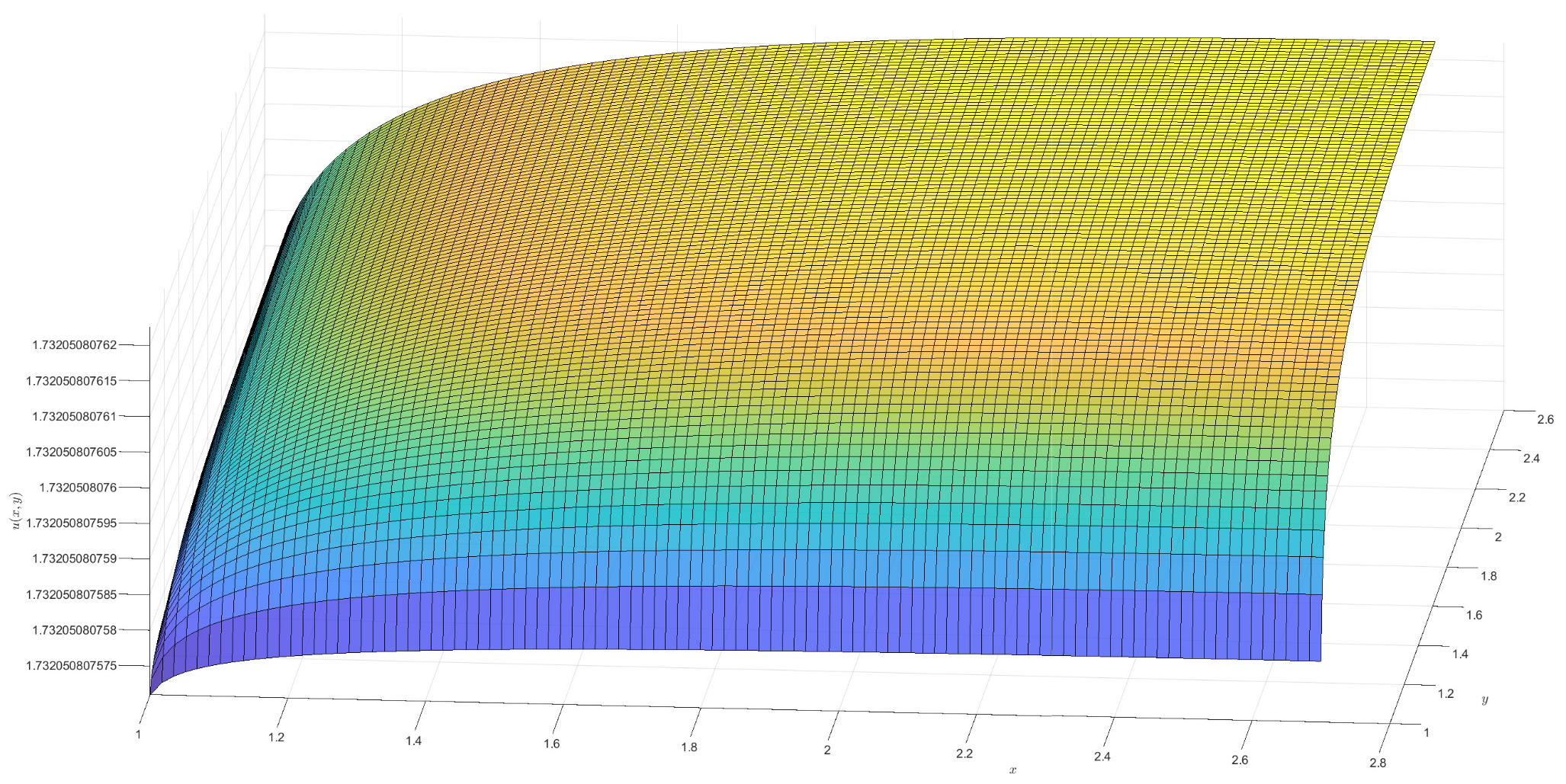
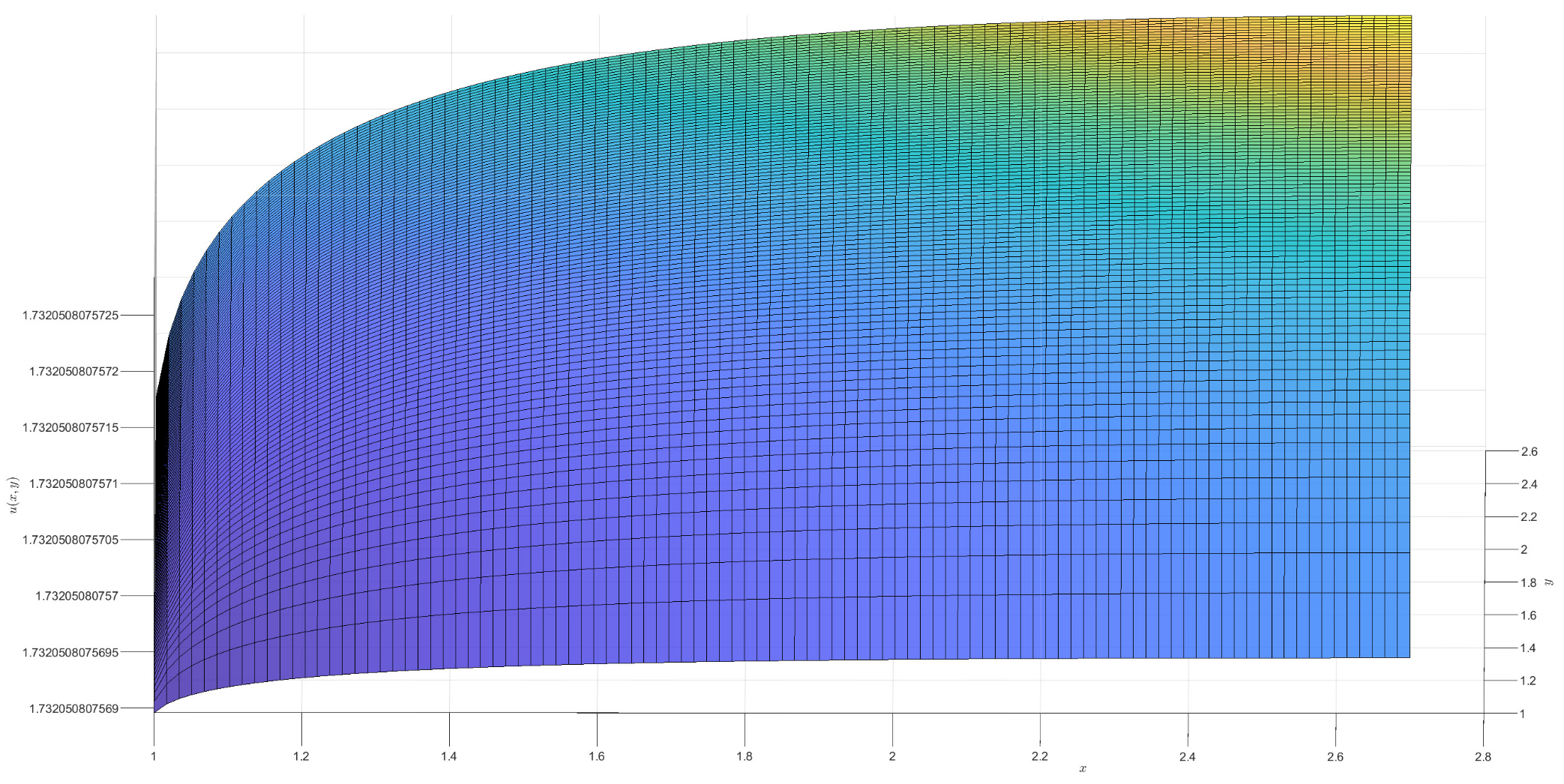
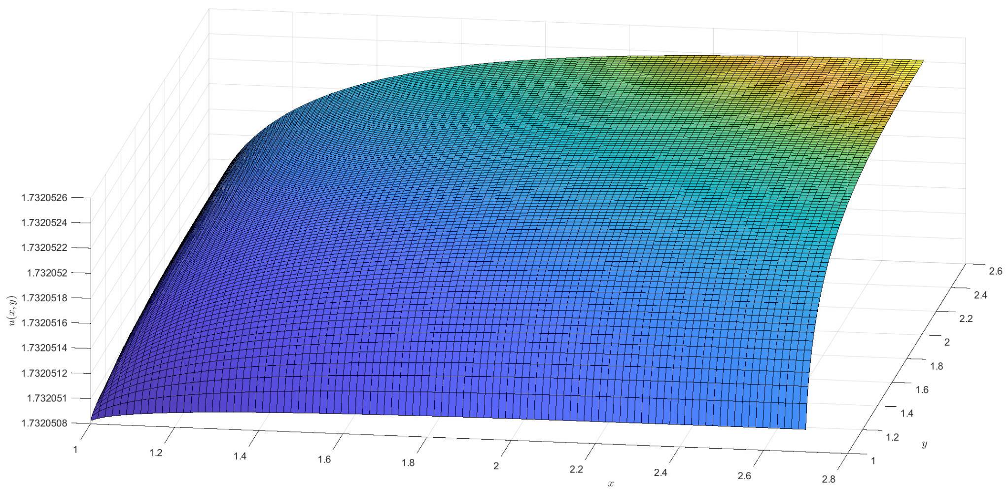
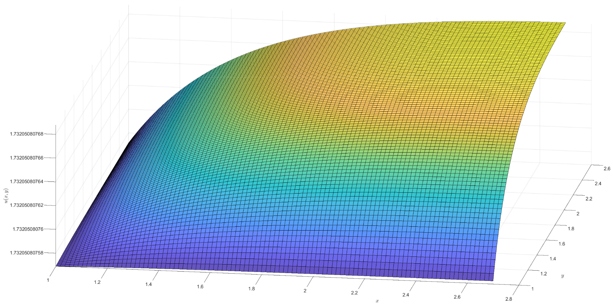
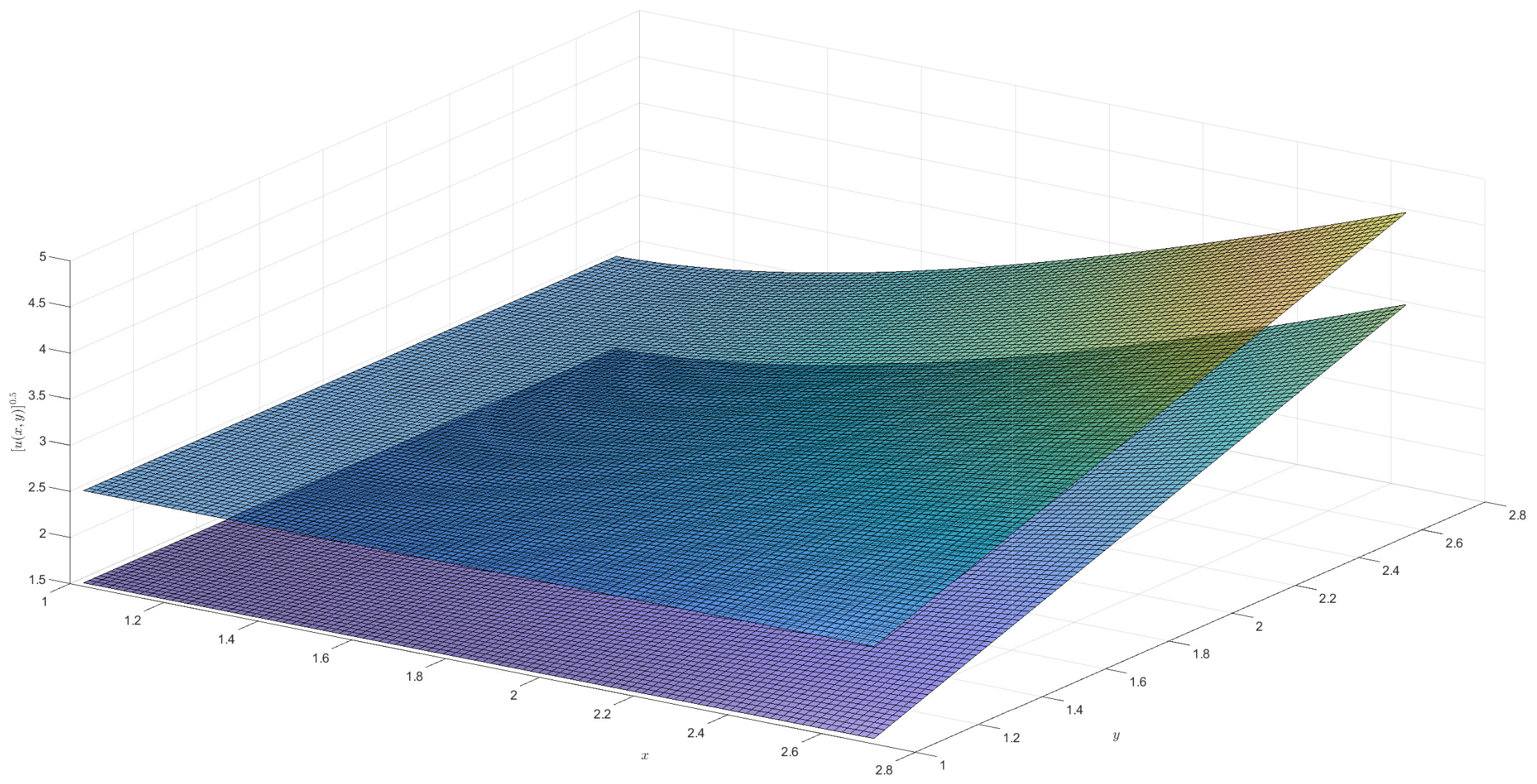
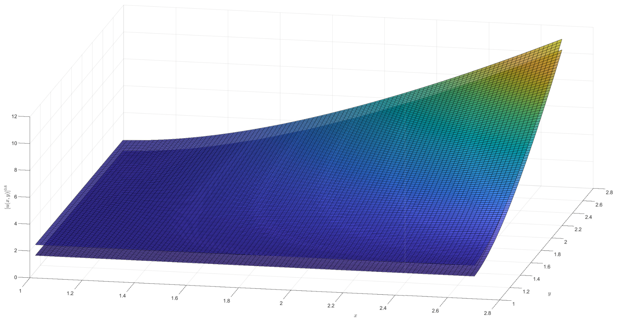
Take $m=100$ and the order of $\theta =0.3,0.4,0.5,1$ ($\theta =1$ is the case of integer-order for (2)). For the †-type solution of different orders in Example 1, numerical integration is utilized to obtain approximate solutions, and 3D visualizations of these approximations are presented (see Figure 1, Figure 2, Figure 3 and Figure 4). Moreover, it can be observed that when $\theta$ is a fractional order ($\theta =0.3,0.4,0.5$), $u(x,y)$ exhibits a broader coverage compared to the integer-order case (i.e., $\theta =1$).

Example 2.

For $i=l=2$, the following Caputo–Hadamard fractional differential equation with a triangular fuzzy number of $M=(1,2,3)$ as the initial value is viewed as follows:

$$\left\{\begin{array}{c}{}_{CH}{}^{\theta }D_{xy}^{2,2}u(x,y)={\displaystyle \frac{\sqrt{7}}{15}}[\log \left(x\right)+\log \left(y\right)],\hfill \\ u(x,y_0)={\varphi }_1\left(x\right)=M,1⩽x⩽e,\hfill \\ u(x_0,y)={\varphi }_2\left(y\right)=M,1⩽y⩽e.\hfill \end{array}\right.$$

(30)

Similarly, we can easily find that Equation (30) satisfies the relevant conditions of Theorem 1 so that (30) has ‡-type solutions ($u(x,y)\in C_{2,2}(\tilde{\mathbf{X}},\mathbb{E})$). Similar to Example 1, we apply a numerical method to show that (30) has a unique solution. Letting $M=(1,2,3)$, it is easy to find that

$${\left[M\right]}^r=\left[{\underline{M}}_r,{\overline{M}}_r\right]=[r+1,3-r].$$

Based on Lemma 6 provided earlier, similar to Example 1, we can obtain the following fuzzy solution:

$$\begin{array}{cc}\hfill u(x,y)& =M\ominus (-1){\displaystyle \frac{\sqrt{7}}{15}}{\displaystyle \frac{1}{\Gamma \left(\theta \right)}}{\displaystyle \frac{1}{\Gamma \left(\theta \right)}}{\int }_1^x{\int }_1^y{\left(\log {\displaystyle \frac{x}{s}}\right)}^{\theta -1}{\left(\log {\displaystyle \frac{y}{t}}\right)}^{\theta -1}{\displaystyle \frac{\log \left(s\right)+\log \left(t\right)}{st}}dsdt.\hfill \end{array}$$

Next, we characterize the existence and uniqueness of solutions to (30) based on the r-level set of the following fuzzy solutions:

$$\begin{array}{cc}\hfill {\left[u(x,y)\right]}^r& =\left[r+1+{\displaystyle \frac{\sqrt{7}}{15}}{\displaystyle \frac{1}{\Gamma \left(\theta \right)}}{\displaystyle \frac{1}{\Gamma \left(\theta \right)}}{\int }_1^x{\int }_1^y{\left(\log {\displaystyle \frac{x}{s}}\right)}^{\theta -1}{\left(\log {\displaystyle \frac{y}{t}}\right)}^{\theta -1}{\displaystyle \frac{\log \left(s\right)+\log \left(t\right)}{st}}dsdt,\right.\hfill \\ \hfill & \left.3-r+{\displaystyle \frac{\sqrt{7}}{15}}{\displaystyle \frac{1}{\Gamma \left(\theta \right)}}{\displaystyle \frac{1}{\Gamma \left(\theta \right)}}{\int }_1^x{\int }_1^y{\left(\log {\displaystyle \frac{x}{s}}\right)}^{\theta -1}{\left(\log {\displaystyle \frac{y}{t}}\right)}^{\theta -1}{\displaystyle \frac{\log \left(s\right)+\log \left(t\right)}{st}}dsdt\right].\hfill \end{array}$$

By utilizing Definition 9, we achieve

$$\begin{array}{cc}\hfill & {\int }_1^{x_{m_1}}{\int }_1^{y_{m_2}}{\left(\log {\displaystyle \frac{x_{m_1}}{s}}\right)}^{\theta -1}{\left(\log {\displaystyle \frac{y_{m_2}}{t}}\right)}^{\theta -1}{\displaystyle \frac{\log \left(s\right)+\log \left(t\right)}{st}}dsdt\hfill \\ \hfill & \approx {\displaystyle \sum _{\ell =0}^{m_1}}{\displaystyle \sum _{j=0}^{m_2}}{\int }_{x_{\ell }}^{x_{\ell +1}}{\int }_{y_j}^{y_{j+1}}{\left(\log {\displaystyle \frac{x_{\ell +1}}{s}}\right)}^{\theta -1}{\left(\log {\displaystyle \frac{y_{j+1}}{t}}\right)}^{\theta -1}{\displaystyle \frac{\log \left(s\right)+\log \left(t\right)}{st}}dsdt,\hfill \end{array}$$

and for $m_1,m_2=1,2,\cdots ,m$,

$$f(s,t)={\left(\log {\displaystyle \frac{x_{\ell +1}}{s}}\right)}^{\theta -1}{\left(\log {\displaystyle \frac{y_{j+1}}{l}}\right)}^{\theta -1}{\displaystyle \frac{\log \left(s\right)+\log \left(t\right)}{st}}.$$

According to (26), for $m_1,m_2=1,2,\cdots ,m$, one can obtain

$$\begin{array}{cc}\hfill {\displaystyle \sum _{\ell =0}^{m_1}}{\displaystyle \sum _{j=0}^{m_2}}& {\int }_{x_{\ell }}^{x_{\ell +1}}{\int }_{y_j}^{y_{j+1}}{\left(\log {\displaystyle \frac{x_{\ell +1}}{s}}\right)}^{\theta -1}{\left(\log {\displaystyle \frac{y_{j+1}}{t}}\right)}^{\theta -1}{\displaystyle \frac{\log \left(s\right)+\log \left(t\right)}{st}}dsdt\hfill \\ \hfill \approx & {\displaystyle \sum _{\ell =0}^{m_1}}{\displaystyle \sum _{j=0}^{m_2}}{\displaystyle \frac{(x_{\ell +1}-x_{\ell })(y_{j+1}-y_j)}{6}}[f(x_{\ell },y_j)+f(x_{\ell },y_{j+1})+f(x_{\ell +1},y_j)\hfill \\ \hfill & +f(x_{\ell +1},y_{j+1})]+4[f\left({\displaystyle \frac{x_{\ell }+x_{\ell +1}}{2}},y_j\right)+f\left({\displaystyle \frac{x_{\ell }+x_{\ell +1}}{2}},y_{j+1}\right)\hfill \\ \hfill & +f\left(x_{\ell },{\displaystyle \frac{y_j+y_{j+1}}{2}}\right)+f\left(x_{\ell +1},{\displaystyle \frac{y_j+y_{j+1}}{2}}\right)]\hfill \\ \hfill & +16\left[f\left({\displaystyle \frac{x_{\ell }+x_{\ell +1}}{2}},{\displaystyle \frac{y_j+y_{j+1}}{2}}\right)\right].\hfill \end{array}$$

(31)

Similar to Example 1, we divide the interval of $[1,e]$ in the same manner, with the set of partition points denoted as $X=\{x_1,x_2,\cdots ,x_m\}$, $Y=\{y_1,y_2,\cdots ,y_m\}$, and the partition distance as $x_{m_1+1}-x_{m_1}=y_{m_2+1}-y_{m_2}={\displaystyle \frac{e-1}{m}}\left(m_1,m_2=1,2,3,\cdots ,m\right)$. Moreover, the computational complexity of (31) is $O\left(m_1{m}_2\right)$. We fix $m=100$ and perform numerical integration at each mesh point, following Definition 9, to compute the approximations. Furthermore, 3D visualizations are generated for different orders on the same level sets (see Figure 5 and Figure 6), as well as for the same order on different level sets (see Figure 7 and Figure 8).

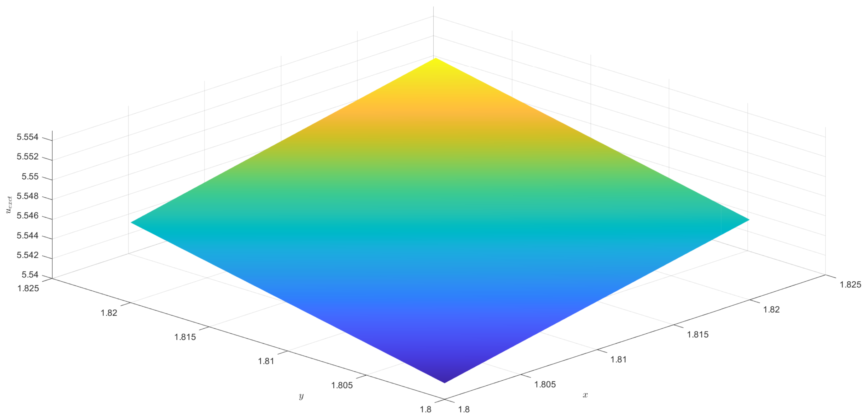
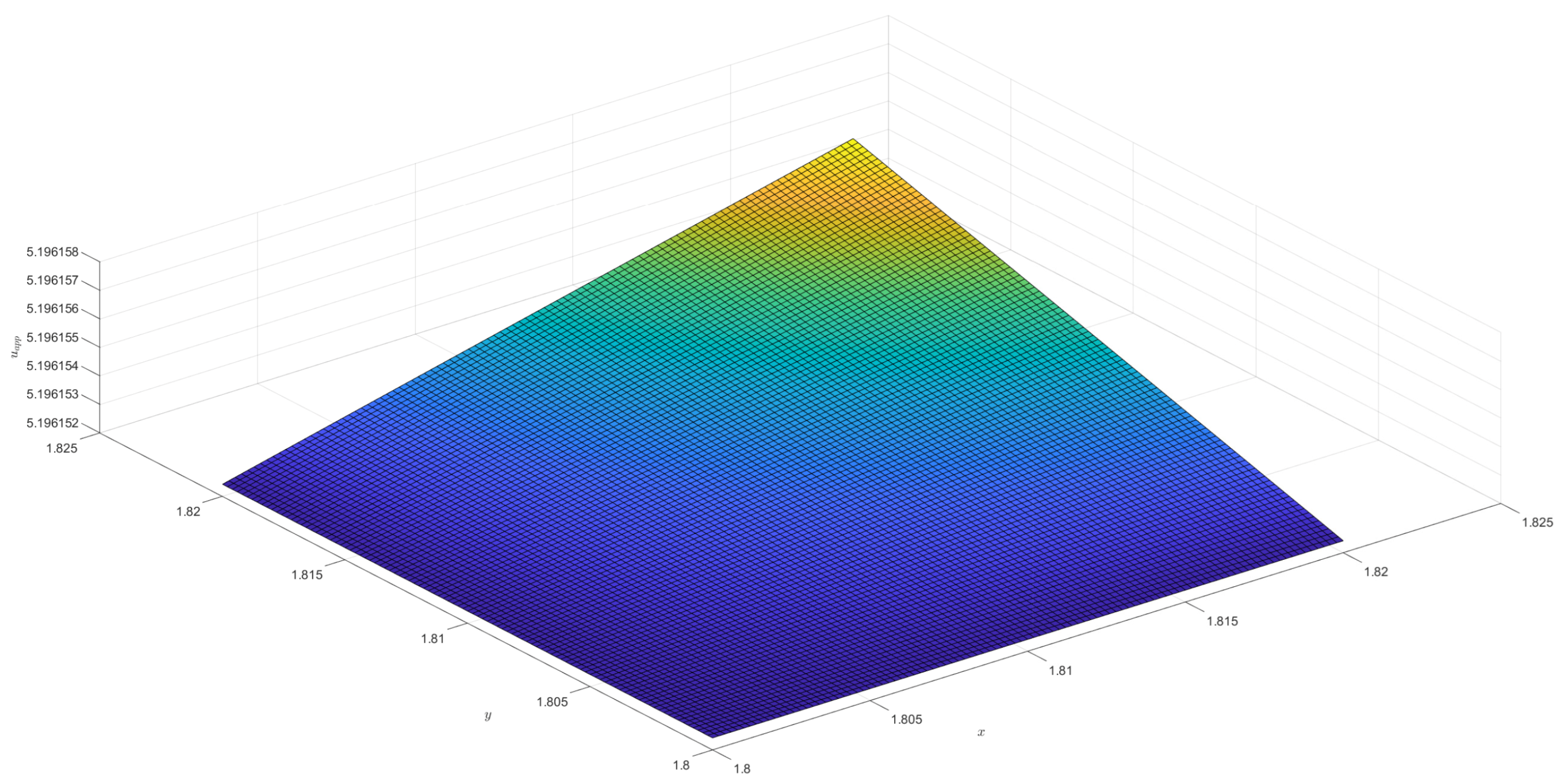
Example 3.

In the special case where $i=l=1$, we consider the following Caputo–Hadamard gH-type fractional differential equation:

$$\left\{\begin{array}{c}{}_{CH}{}^{\theta }D_{xy}^{1,1}u(x,y)={\displaystyle \frac{4}{\pi }}{\left(\log x\right)}^{0.5}{\left(\log y\right)}^{0.5},\hfill \\ u(x,y_0)={\varphi }_1\left(x\right)=3\sqrt{3},1.8⩽x⩽1.82,\hfill \\ u(x_0,y)={\varphi }_2\left(y\right)=3\sqrt{3},1.8⩽y⩽1.82.\hfill \end{array}\right.$$

(32)

Similar to Example 1, it can be shown that (32) admits †-type solutions ($u(x,y)\in C_{1,1}(\widehat{\mathbf{X}},\mathbb{E})$, where $\widehat{\mathbf{X}}=[1.8,1.82]\times [1.8,1.82]$); furthermore, $u(x,y)=3\sqrt{3}+\log x\log y$. In the following, we employ a numerical approximation method analogous to that used in Example 1 to compute an approximate solution of (32). Similar to Example 1, we divide the interval of $[1.8,1.82]$ in the same manner, with the set of partition points denoted as $X=\{x_1,x_2,\cdots ,x_{100}\}$, $Y=\{y_1,y_2,\cdots ,y_{100}\}$, and the partition distance as $x_{m_1+1}-x_m=y_{m_2+1}-y_{m_2}=0.0002$ $\left(m_1,m_2=1,2,3,\cdots ,100\right)$. We obtain the following numerical approximation for $u(x,y)$.

$$\begin{array}{cc}\hfill u(x_{m_1},y_{m_2})\approx & 3\sqrt{3}+{\displaystyle \frac{{\left(0.0001\right)}^2}{{\pi }^2}}{\displaystyle \sum _{\ell =1}^{m_1}}\left[{\left({\displaystyle \frac{ln{x}_{\ell }}{ln{x}_{\ell -1}}}\right)}^{-0.5}{\displaystyle \frac{{(ln{x}_{\ell -1})}^{0.5}}{x_{\ell }}}\right]\hfill \\ \hfill & {\displaystyle \sum _{j=1}^{m_2}}\left[{\left({\displaystyle \frac{ln{y}_j}{ln{y}_{j-1}}}\right)}^{-0.5}{\displaystyle \frac{{(ln{y}_{j-1})}^{0.5}}{y_j}}\right].\hfill \end{array}$$

Subsequently, the exact solution of (32) is presented and illustrated in Figure 9, where $u_{exct}(x,y)$ denotes the exact solution. The corresponding numerical approximation, denoted by $u_{app}(x,y)$, is shown in Figure 10. Furthermore, the relative error between the numerical and exact solutions, denoted by $u_{▵}(x,y)={\displaystyle \frac{|u_{exct}(x,y)-u_{app}(x,y)|}{u_{exct}(x,y)}}$, is depicted in Figure 11, which further demonstrates the accuracy and validity of the numerical method.

Remark 6.

For Example 1, the computational complexity associated with the application of the trapezoidal rule, as presented in (28), is represented by $O(m_1+m_2)$. In Example 2, the computational complexity of applying Simpson’s rule as described in (31) is denoted by $O\left(m_1{m}_2\right)$. In practical applications, on the one hand, FFPDE models often involve more than two variables; on the other hand, achieving accurate approximations typically requires finer partitioning of the domain. Both factors contribute to an increase in computational complexity. For example, in Example 1, when the number of variables increases to $m_k$ ($m_k>2$), the computational complexity of (28) also increases to $O(m_1+m_2+···+m_k)$. In Example 2, a finer partitioning of the domain (i.e., a significant increase in $m_1$ and $m_2$) leads to a significant increase in the computational complexity ($O\left(m_1{m}_2\right)$) associated with (31).

5. Concluding Remarks

The primary purpose of this paper is to focus on the existence and uniqueness of solutions for the following FFPDE of Caputo–Hadamard-type derivative involving gH difference under some suitable conditions:

$$\left\{\begin{array}{c}{}_{CH}{}^{\theta }D_{xy}^{i,l}u(x,y)=a_1{}_{CH}{}^{\theta }D_x^{i}u(x,y)+a_2{}_{CH}{}^{\theta }D_y^{1}u(x,y)+a_{3}u(x,y)+a_{4}G(x,y),\hfill \\ u(x,y_0)={\varphi }_1\left(x\right),x_0\le x\le T,\hfill \\ u(x_0,y)={\varphi }_2\left(y\right),y_0\le y\le T,\hfill \end{array}\right.$$

(33)

The classic Caputo FDE had been innovatively extended to a Caputo–Hadamard FDE, which holds significant meaning due to its integral kernel being in the form of a logarithm rather than the traditional sense of subtraction.

Building upon the work of previous researchers, the main innovations and objectives of this paper are outlined as follows:

(i) In the context of Goursat problems, we extend traditional Caputo FDEs to Caputo–Hadamard FDEs, thereby altering the form of the integral kernel.

(ii) We establish the uniqueness and existence of solutions to problem (33) using the Banach fixed-point theorem and Schauder fixed-point theorem. This has not yet been reported in the literature.

(iii) We present relevant numerical examples used in the existence and uniqueness results and further obtain an approximate numerical solution for (33) by discretizing $u(x,y)$.

As mentioned in Remark 1 (i), it is worth exploring the application of the model (2) (i.e., FFPDE (33)) in circuit design and communication in the future. Furthermore, in disciplines such as finance, operations research, optics, medicine, biology, engineering, and other practical applications, time delays and pulse effects often arise due to instrumental measurements or human interventions. A valuable potential direction for future work is to investigate whether the solution of (33) maintains its existence and uniqueness under time delay $(x-t,y-\sigma )$ and during the occurrence of the pulse phenomena.

On the other hand, it is worth investigating whether existing methods for solving FDEs can enhance the accuracy of the numerical solutions for the proposed FFPDE model. As reported by Desiderio et al. [42], for large-scale practical simulations, the limitations of current computing resources make it difficult to solve the corresponding systems on standard personal computers. Given these challenges, the combination of hierarchical matrices ($\mathcal{H}$ matrix) [43] and Adaptive Cross Approximation (ACA) [44] offers a promising approach for practical problems. In fact, several researchers have successfully applied such methods and obtained favorable results. For example, Chaillat et al. [45] investigated fast H-matrix based methods for solving dense linear systems arising from the discretization of 3D elastodynamic Green tensors, demonstrating both accuracy and efficiency. Aimi et al. [46] studied acoustic and elastic wave propagation in unbounded two-dimensional domains and reformulated the problems as space–time boundary integral equations. Desiderio et al. [42] considered interior and exterior three-dimensional Helmholtz problems, also reformulated as boundary integral equations. Such methods include the variational iteration method and Adomian decomposition method proposed by Odibat et al. [47], the adaptive predictor–corrector algorithm introduced by Sadek et al. [48], and the meshless generalized finite difference method based on moving least squares developed by Garcia et al. [49], among others. In addition, how these numerical approaches can be adapted to effectively handle the FFPDE system with Caputo–Hadamard derivatives presented in this study remains a meaningful and challenging problem for future research.