Article

Long-Term Persistence in Observed Temperature and Precipitation Series

by
Huayu Zhong
1,2 and
Yiping Guo
2,*
1
College of Water Conservancy and Hydropower Engineering, Hohai University, Nanjing 210098, China
2
Department of Civil Engineering, McMaster University, Hamilton, ON L8S 4L8, Canada
*
Author to whom correspondence should be addressed.
Fractal Fract. 2025, 9(6), 385; https://doi.org/10.3390/fractalfract9060385
Submission received: 6 May 2025 / Revised: 9 June 2025 / Accepted: 13 June 2025 / Published: 17 June 2025

Abstract

The Hurst phenomenon is regarded as an intrinsic characteristic of many natural processes closely related to high uncertainty and long-term persistence. Temperature and precipitation are the two important meteorological factors characterizing the climate conditions of different regions. Analyzing the Hurst phenomenon in precipitation and temperature are crucial for understanding the long-term dynamics of our climate system. This study examines the annual mean temperature (AMT) and annual total precipitation (ATP) series for regions across all the land areas of the world, using both gridded climate data and ground station records. The results demonstrate that, in most regions, the Hurst exponent of AMT is higher than that of ATP, particularly with larger spatial scales of averaging. Like ATP, the Hurst exponents of AMT also increase with the spatial scale of averaging. Unlike AMT, ATP is more controlled by local meteorological conditions which tend to weaken its long-term persistence. Moreover, the cumulative departure from the mean series of ATP is much more variable across different regions, whereas those of AMT for different regions are more similar. What is identified for the first time in this study is the strong similarity in the cumulative departure from the mean patterns of regionally averaged and individual stations’ ATP and AMT series over many regions of the world. At most of these regions and stations where such similarities are identified, more than half have confirmed that AMT is the Granger cause of ATP variations. Moreover, the fluctuation functions obtained in multifractal detrended cross-correlation analysis exhibit approximately linear behavior in the log–log spaces across all regions at both global and continental scales, indicating that ATP and AMT series are long-range cross-correlated.

1. Introduction

Long-term persistence (LTP), also known as long-range dependence, long-memory or Hurst–Kolmogorov dynamics in geophysical time series (GTS) was first discovered by Hurst [1,2], and the statistic he used to quantify it was later known as the Hurst exponent or Hurst coefficient. The Hurst exponent (denoted as H) can have values ranging from 0 to 1. When the H value of a GTS is greater than 0.5, it exhibits LTP. Hurst calculated the H values for a large number of GTS such as river flows, rainfall, temperature, tree rings, and lake levels [2]. He found that the average H value of these GTS was 0.73, indicating a significant presence of LTP. In particular, Hurst reported that the H value for the annual streamflow of the Nile River at Aswan was 0.9, demonstrating even a stronger LTP. Similarly to other GTS, if the Nile River’s annual flow series is serially independent white noises, its H should be 0.5. This inconsistency between theory and observation led subsequent researchers to name this somewhat strange phenomenon the Hurst phenomenon [3,4,5,6].
Hurst himself noted that “Although clusters of high or low values occur in random events, their tendency to occur is stronger in natural events [1]. This is the main difference between natural and random events”. The observed Hurst phenomenon suggests that, in many GTS, high values tend to follow high values and low values tend to follow low values. This non-randomness or LTP is also reflected in the fact that the autocorrelation functions of the many GTS decay slowly according to a power law, whereas exponential decay is expected for stationary time series with correlation between consecutive observations not persisting over long lags. Traditional modeling approaches based on the principle of independence among consecutive observations or stationary processes with short memories may not accurately describe some natural phenomena [7,8,9].
Ever since the Hurst phenomenon was introduced into the scientific discourse in the 1950s, interest in this time series behavior has been steadily increasing. Researchers all over the world have devoted more and more efforts to discover and explain the Hurst phenomenon in different GTS [10]. The Hurst phenomenon has been identified in many hydrological and meteorological records, including precipitation [6,11,12,13,14], streamflow [15,16,17], air temperature [4,18,19], wind energy [20,21], groundwater level [22], evapotranspiration [23], and solar radiation [24]. Its importance has also been recognized in various other fields such as economics and finance [25,26], medicine [27], and ecology [28]. The implications of the Hurst phenomenon are significant for both research and practical applications.
As a crucial variable within the climate system, annual total precipitation (ATP) has a profound impact on ecosystems, agricultural productivity, and human society [29]. ATP is typically controlled by various meteorological factors and exhibits complex fluctuation patterns, making its changes challenging to predict accurately [30,31]. Despite the significant uncertainty in its long-term variations, ATP’s fluctuation patterns display clear self-similarity or equivalently LTP, implying that past ATP may impact current ATP [32,33]. This characteristic has spurred extensive global research into the presence of the Hurst phenomenon in ATP. Evidence confirming the Hurst phenomenon in ATP has emerged from various regions [34,35,36,37]. The exact H values of the ATP series were found to be influenced by various factors such as station location [14], climate type [38], temporal scale of aggregation [39], station elevation [40], and the length of historical records [35,41]. Studies conducted before 2023 concluded that the Hurst phenomenon in ATP at ground stations and grids was relatively weak, with the average or median H value ranging between 0.6 and 0.7 [6,13,41].
For the first time, O’Connell et al. discovered that the weaker LTP of local ATP is primarily a result of local climate variability, which may be thought of as the noises added to larger spatial scale precipitation patterns [6]. As precipitation is averaged over larger spatial scales, the local variability or noises are gradually smoothed or canceled out, resulting in a significant enhancement of LTP at the regional scale. Their analysis of gridded and spatially averaged ATP data from eight regions worldwide showed that the mean H value at the grid scale was 0.66, which increased to 0.83 at the regional scale.
Fractal and multifractal analyses have been widely applied to characterize the nonlinear and scale-dependent behavior of precipitation and temperature across different climatic regimes. Rainfall time series, particularly at daily or sub-hourly scales, often exhibit multifractal properties and long-range persistence, consistent with multiplicative cascade processes and atmospheric intermittency [42,43,44,45]. In drought-prone or convective-dominated regions, the irregular alternation of wet and dry spells has been analogized to the Cantor set—a classical fractal structure characterized by recursive gaps—capturing the fragmented and clustered nature of precipitation under extreme conditions [46,47,48]. Tools such as fractal dimensions, lacunarity analysis, and the Hurst exponent have been widely used to quantify precipitation persistence, variability, and temporal organization [6,49]. From a theoretical perspective, recent advances in chaos theory and fractal geometry, including the application of Julia sets and memristor-based attractor systems, offer insight into the underlying nonlinear dynamics that govern hydroclimatic time series [50,51,52]. These advances jointly illustrate and emphasize the importance of incorporating both statistical and geometric approaches to better understand the coupled long-term memory of temperature and precipitation in a changing climate.
Temperature is another key atmospheric factor; its variations exert significant impacts on the environment, ecosystems, production, and daily life [53,54,55]. Climate change, characterized primarily by global warming, is one of the most pressing environmental challenges facing the world today [56,57,58,59]. Numerous scientific studies have extensively confirmed the profound impacts of rising global temperatures, including the increased frequency of extreme weather events, rising sea levels, and significant changes in ecosystems [60,61,62]. However, despite these studies underscoring the importance of understanding temperature changes, research on whether Hurst phenomena exist in point or regionally averaged annual mean temperature (AMT) series has been relatively limited. Koutsoyiannis found that the 231-year-long AMT series at Paris has an H value of 0.79 and the 992-year long-AMT series of the Northern Hemisphere (obtained by using temperature-sensitive paleoclimatic multi-proxy data) has an H value of 0.86 [4]. Using the classical rescaled range analysis method, Hamed found that the AMT series at 36 out of 56 individual stations in the Midwest USA exhibit the Hurst effect and the average of the H values at the 36 stations was found to be 0.73 [19]. The lengths of the AMT series analyzed by Hamed range from 68 to 107 years. Glynis et al. (2021) analyzed the AMT data from 245 global stations and found an average H value of 0.75, with the AMT series lengths ranging from 83 to 136 years [18]. These studies seem to indicate that AMT has relatively high H values, and its Hurst phenomenon appears to be more pronounced than that of ATP discussed earlier. However, current research lacks sufficient evidence to fully support this hypothesis. Furthermore, whether AMT exhibits spatial dependence similar to ATP is a question that merits further exploration.
The water vapor content in the atmosphere is the principal driver of precipitation [63,64] and temperature has a significant effect on it [65]. Under conditions of nearly constant relative humidity, the rate of water vapor growth is closely related to temperature and follows the Clausius–Clapeyron equation, with water vapor content increasing by approximately 7% per Kelvin in the troposphere [66]. Since ATP variations are primarily driven by the supply of water and energy, which are closely related to temperature, changes in precipitation patterns are largely controlled by changes in AMT. Globally, ATP generally increases with rising AMT [67]. Through analysis of streamflow data from 39 European rivers, the higher temperatures (particularly in areas with minimal snowmelt) resulted in stronger streamflow LTP as reflected in increased H values [68]. Additionally, O’Connell et al. also demonstrated that the LTP in the annual flows of the Nile River at Aswan can be attributed to the LTP in its basin-averaged ATP [6]. Since the relationship between AMT and ATP for different locations is very complex and is difficult to ascertain, especially under changing climate conditions, for a long time there has been debate over whether the Hurst phenomenon in AMT is the cause of the Hurst phenomenon in ATP.
Both thermodynamic and kinetic factors contribute to the variability of precipitation [69,70,71], complicating efforts to ascertain whether the Hurst phenomenon in ATP is indeed AMT-driven. Although it is unequivocal that AMT is a significant meteorological factor affecting the variability in ATP, so far no one has provided definitive evidence confirming that the Hurst phenomenon in ATP is caused by the Hurst phenomenon in AMT. In this study, both ATP and AMT series for locations all over the world were collected and analyzed. Spatially averaged ATP and AMT series were obtained for different regions across the globe. O’Connell et al.’s recent finding that the H values of ATP increase with the spatial scale of averaging is confirmed again by our analysis [6]. We also report new findings that the H values of AMT increase as well with the spatial scale of averaging and the H values of AMT are always higher than the H values of ATP. Meanwhile, over many subregions, the cumulative departures from the means of regionally averaged ATP series were found to fluctuate very similarly to those of the regionally averaged AMT series. This similarity was discovered for the first time and led us to hypothesize that the Hurst phenomenon in the AMT may be one of the main causes of the Hurst phenomenon in ATP. Granger causality tests and multifractal detrended cross-correlation analyses were conducted to verify this newly hypothesized causal relationship between AMT and ATP.

2. Data and Methods

2.1. Meteorological Data and Regions Analyzed

To ensure robust and accurate estimation of the Hurst exponent, Markonis and Koutsoyiannis advocate for a sample size of at least 100 when evaluating the Hurst behavior of annual precipitation [41]. The Climatic Research Unit (CRU)’s time series data are one of the most widely used climate datasets produced by the United Kingdom’s National Centre for Atmospheric Science [72]. It provides monthly climate data for the global land surface from 1901 to 2023 with a spatial resolution of 0.5°. The dataset includes the following 10 variables based on near-surface measurements: temperature (mean, minimum, maximum, and diurnal temperature range), precipitation (total and wet-day count), humidity (such as vapor pressure), frost days, cloud cover, and potential evapotranspiration. This study utilized the CRU’s gridded monthly precipitation and temperature data (https://crudata.uea.ac.uk/cru/data/hrg/, accessed on 1 December 2024). We focused on the Hurst exponent of precipitation and temperature on an annual scale as well as the correlation between them. To achieve this, ATP was obtained by summing the monthly precipitation, while the AMT was calculated by averaging the monthly temperature throughout the year.
Moreover, since raster data were obtained from actual observations at individual ground monitoring stations, their accuracy is closely linked to the density of these stations. To further validate our research conclusions, we downloaded precipitation and temperature data from 45 ground meteorological stations in China, the United States, and the United Kingdom for additional analysis. The observational data from China and the United States were obtained from NOAA (https://www.ncei.noaa.gov/cdo-web/, accessed on 1 December 2024), while the data from the United Kingdom came from the UK Meteorological Office (https://www.metoffice.gov.uk/research/climate/maps-and-data/historic-station-data, accessed on 1 December 2024). Monthly precipitation and monthly average temperature were also processed to obtain ATP and AMT series. These websites were accessed on 1 December 2024.
Spatial averaging of meteorological data can affect calculation results [6]. To analyze the impact of spatial averaging on ATP and AMT, this study applied two regional division methods. The first method is based on continents, where the global gridded data provided by the CRU are averaged for each continent. Since the CRU data do not include Antarctica, this region was excluded from the analysis. Additionally, considering the scattered land distribution in Oceania, which could affect significantly the results, only Australia was selected for spatial averaging in this region. The second method is more refined, using the regional division standard of the Intergovernmental Panel on Climate Change (IPCC)’s Sixth Assessment Report (AR6), which divides global land areas into 46 subregions (https://www.ipcc.ch/report/ar6/syr/, accessed on 1 December 2024). These subregions cover all global land areas and are designed in a rectangular shape to facilitate spatial aggregation analysis (shown in Figure 1). In actual calculations, the regionmask.defined_regions.ar6.land function in Python 3.12.0 was used to implement this division. Since EAN and WAN are located in Antarctica, the CRU data were ultimately divided into 44 subregions.

2.2. Estimation of the Hurst Exponent

The Hurst exponent (H) was first introduced by Harold Edwin Hurst to determine the optimal dam size based on fluctuations of Nile River’s water levels [2]. This exponent quantifies the extent to which past values influence the future trend of a time series and is commonly used to characterize LTP. Specifically, 0.5 < H < 1 indicates persistence, meaning that past trends are likely to continue (long-term positive correlation); 0 < H < 0.5 suggests anti-persistence, where an increase is more likely to be followed by a decrease (long-term negative correlation) in trends; and H = 0.5 corresponds to a purely random, memoryless process.
Various methods have been developed to estimate the H value. Among them, the R/S analysis method, one of the earliest and widely used tool for H value estimation, continues to attract attention due to its relevance to practical applications [19]. Although studies have shown that the R/S method can produce biased H estimates—overestimating H for time series with H < 0.7 and underestimating it for those with H > 0.7 [73]—it remains the most commonly used approach for evaluating H values in hydrological time series. As such, this study adopted the non-parametric R/S analysis method to estimate the H values, serving as a reference for confirmation and validation purposes [2]. In using the R/S method, the sample series is divided into segments of varying lengths. For each segment, the cumulative deviation from the mean is calculated. The range R of these cumulative deviations is then determined and normalized by dividing it by the standard deviation S of the segment:
R S = max X t min X t S
where Xt represents cumulative deviations within each segment. By plotting the rescaled range R/S against the segment length on a log–log scale, the slope of the resulting line estimates the Hurst exponent H, typically through the following relation:
log R / S n = H · log n + log c
where n is the segment length and c is a constant.
To accurately estimate the H value of a time series, Serinaldi evaluated several commonly used estimation methods using both real-world observational data and synthetic series generated from fractional Gaussian noise (fGn) and fractional Brownian motion (fBm) models [74]. It was observed that the R/S method is effective for fGn-type signals but unsuitable for fBm-type signals, for which it tends to overestimate H. Detrended fluctuation analysis (DFA) is more accurate for the fBm-type series but often underestimates H when applied to the fGn-type series. Power spectral density (PSD) analysis can be used for both fGn and fBm, but its performance deteriorates when β < −2 or β > 4, exhibiting high bias and variance. Here β, the power spectral exponent, is directly related to the H values for stationary processes. Serinaldi provides details of all seven compared H estimation methods and cautioned that selecting an appropriate method is critical for accurately estimating H in a time series [74].
To this end, we employed the Whittle maximum likelihood estimation (WMLE) method to estimate the H for fGn-type series. This method has been widely recognized as one of the most accurate technique for estimating H [19,75]. The WMLE is formulated as an optimization problem, where the objective is to estimate H by maximizing Whittle’s log-likelihood function lW (H) defined as
l W H = 2 N j = 1 m ln c T ω j ; H + P ω j c T ω j ; H
where m is the integer part of (N − 1)/2; ωj with j = 1, 2, …, m are the Fourier frequencies defined as ωj = 2πj/N; P(ωj) is the periodogram of the observation vector x(j) of length N; T’(ωj; H) is the theoretical power spectral density of the modeled process with parameter H; c is a constant of proportionality used to adjust the power T’(ωj; H) to that of P(ωj); and H is the Hurst exponent in the range of [0, 1]. The mathematical formulation and implementation details of the WMLE method are described in detail in the work of [76].
By contrast, DFA is widely regarded as a reliable method for estimating H in fBm-type processes. It overcomes the limitations of traditional methods by accounting for local trends at various time scale. In this study, the DFA method was used to estimate the H values of fBm-type series. Furthermore, Qian et al. demonstrated DFA’s superior performance in determining the H values if it is combined with empirical mode decomposition (EMD) [77].
To obtain the most accurate estimates of the H values for both the ATP and AMT series, this study uses the WMLE method if a series is confirmed to be an fGn series, and the EMD-DFA method if it is identified as an fBm series. Specifically, the WMLE method was used first to calculate the H values for ATP and AMT. If the H value was found to exceed 0.9998, the series was regarded as a possible fBm series. Its spectral exponent β was then calculated using the PSD method. If β > 1, the series was confirmed to be an fBm series, its H value was recalculated using EMD-DFA. The PSD method is commonly employed to distinguish between time series types (fBm or fGn) [74,78]. For simplicity in the subsequent discussion, we refer to the method used in this study, which combines WMLE and EMD-DFA to calculate the H values of the ATP and AMT series as the WMLE–EMD-DFA method.

2.3. Regional Averaging Considering Different Grid Cell Sizes

When analyzing gridded precipitation data from the Global Precipitation Climatology Centre (GPCC), O’Connell et al. reported that as the scale for spatial averaging increases, the H values of precipitation gradually increase as well [6,12]. Therefore, it is particularly important to investigate whether the CRU precipitation and temperature data also exhibit a similar spatial scale dependency. This study resampled the global grid data of ATP and AMT from the original resolution of 0.5° × 0.5° to four coarser resolutions: 2.5° × 2.5°, 5° × 5°, 7.5° × 7.5°, and 10° × 10°. Resampling was performed by spatial aggregation, calculating the average of all the 0.5°-grid values within each coarser grid cell to obtain more spatially averaged characteristics [79]. The H values of ATP and AMT were calculated later for each aggregated resolution. By comparing the H values of ATP and AMT across all grid points at different spatial resolutions, we can clearly observe whether they exhibit spatial scale dependency or not.
Furthermore, based on the two regional division methods introduced in Section 2.1, we calculated the regional mean values of ATP and AMT, as well as their corresponding H values for all the regions. By comparing the median H values of grid points within each region with the H values of the regionally averaged ATP and AMT series, we further assessed whether the H values of ATP and AMT demonstrate spatial scale dependencies.
It is also important to note that the original spatial resolution of the CRU data is 0.5° × 0.5°, but each grid cell’s area varies with latitude. Grid cells closer to the equator cover larger areas; for example, grid cells in northern Asia are approximately one-fourth of the areas of those at the equator. When calculating the regional mean ATP or AMT values, it is necessary to account for differences in grid cell areas. In this study, we applied Formula 1 from [80] to calculate the projected surface area of each 0.5°-grid cell in the CRU dataset, ensuring accurate regional averaging.

2.4. Analysis of CDM Plots

The cumulative departure from the mean (CDM) plot is a valuable diagnostic tool that can help reveal potential trends in a time series, and the intensities of these trends are reflected in the Hurst exponent. The CDM of a time series Xt with t = 1, 2, …, n is defined as
C D M k = k = 1 n X t k X ¯
where CDMk is the CDM at time point k, 1 ≤ kn where n is the length of the time series, and X ¯ is the mean. O’Connell et al. demonstrated, through analyzing the behaviors of the CDM plots of precipitation and runoff, that the Hurst phenomenon of the annual Nile River flow at Aswan originates from the Hurst phenomenon of the annual precipitation in the Blue Nile Basin [6].

2.5. Regression Analysis Identifying Relative Subarea Contributions

Stepwise linear regression is utilized to evaluate the contributions of ATP or AMT from various subregions to the ATP or AMT of a larger region. This method selectively identifies the most statistically significant subregional contributors, iteratively refining the model by including or excluding variables based on their contributions to the overall regional ATP or AMT. This analysis aids in isolating key subregional influences, enhancing the interpretive clarity of each area’s impact.

2.6. Granger Causality Tests and Multifractal Detrended Cross-Correlation Analyses

To assess the causal influence between the ATP and AMT time series, we employed the classical Granger causality test [81]. This test is based on a Vector Autoregressive (VAR) framework, in which ATP is regressed on its own past values and those of AMT. An F-test is then conducted to compare the unrestricted model (including lagged AMT terms) with a restricted model (excluding lagged AMT terms). If the inclusion of AMT significantly reduces the residual sum of squares, the F-statistic becomes large and the corresponding p-value falls below the significance level (typically 0.05), indicating that AMT Granger causes ATP. Otherwise, the null hypothesis of no causality cannot be rejected. The optimal lag order p was selected using the Akaike Information Criterion (AIC) and Schwarz Criterion (SC), ensuring a balance between model complexity and predictive performance.
Multifractal detrended cross-correlation analysis (MF-DCCA) as described by [82] was also conducted for the global and continental ATP and AMT series to examine the long-range cross-correlations between the two time series. MF-DCCA has been widely applied to investigate the correlations among meteorological variables. For example, it was employed in [83] to examine the multifractal cross-correlations between meteorological parameters and air pollution, and in [84] to explore the relationship between sunspot numbers and river flow fluctuations from a multifractal perspective.

3. Results

3.1. Hurst Exponents of the Gridded and Station ATP and AMT Series

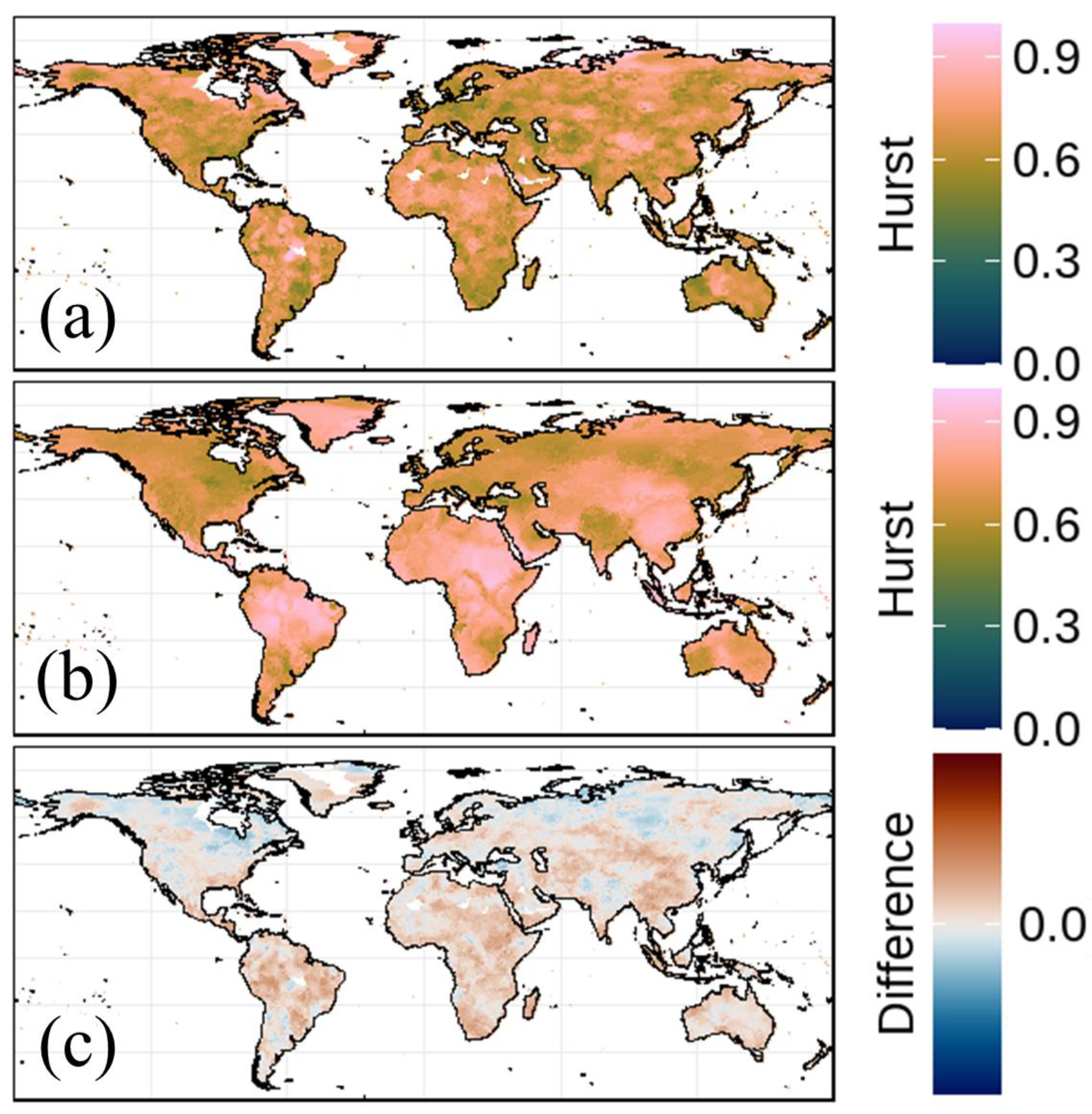
Using WMLE–EMD-DFA method, we calculated the H values for ATP and AMT at all land surface grid points based on gridded data from the CRU. The results are summarized in Figure 2. Figure 2a illustrates the global distribution of the H values for ATP, revealing that 81% of the grid points have H values exceeding 0.5. Notably, 34% of these points, primarily concentrated in northeastern North America, large parts of South America, North Africa, and northern Asia, have H values exceeding 0.7. Figure 2b presents the global distribution of the H values for AMT, where 93% of the grid points have H values surpassing 0.5, with approximately 82% exceeding 0.7. Unlike ATP, AMT exhibits consistently strong LTP across the globe. The differences between the H values of AMT and ATP are depicted in Figure 2c, where positive values indicate that AMT has a higher H value than that of ATP, while negative values signify the opposite. Among all grid points, 83% show higher H values in AMT than in ATP. These differences are generally substantial, with a mean value of 0.25. In contrast, approximately 17% of the grid points exhibit higher H values in ATP than in AMT, these differences tend to be minor, with a mean value of only 0.11.
We performed the same calculations using the R/S analysis method as well, the results are presented in Figure 3. Figure 3a displays the global distribution of the H values for ATP, showing that nearly all grid points have H values exceeding 0.5, and 47% of these points have values above 0.7. In contrast, Figure 3b shows the global distribution of the H values for AMT, where over 99% of the grid points have H values surpassing 0.5, with approximately 64% exceeding 0.7. Figure 3c illustrates the differences in the H values between AMT and ATP, revealing that 65% of the grid points exhibit higher H values for AMT than for ATP. In addition, although approximately 35% of the grid points showed higher H value for ATP than for AMT, the differences in H values for these grid points were generally small, with a mean difference of only 0.07. Overall, regardless of the method used to estimate the H values of ATP and AMT in global gridded data, AMT always exhibits a higher H value than ATP.
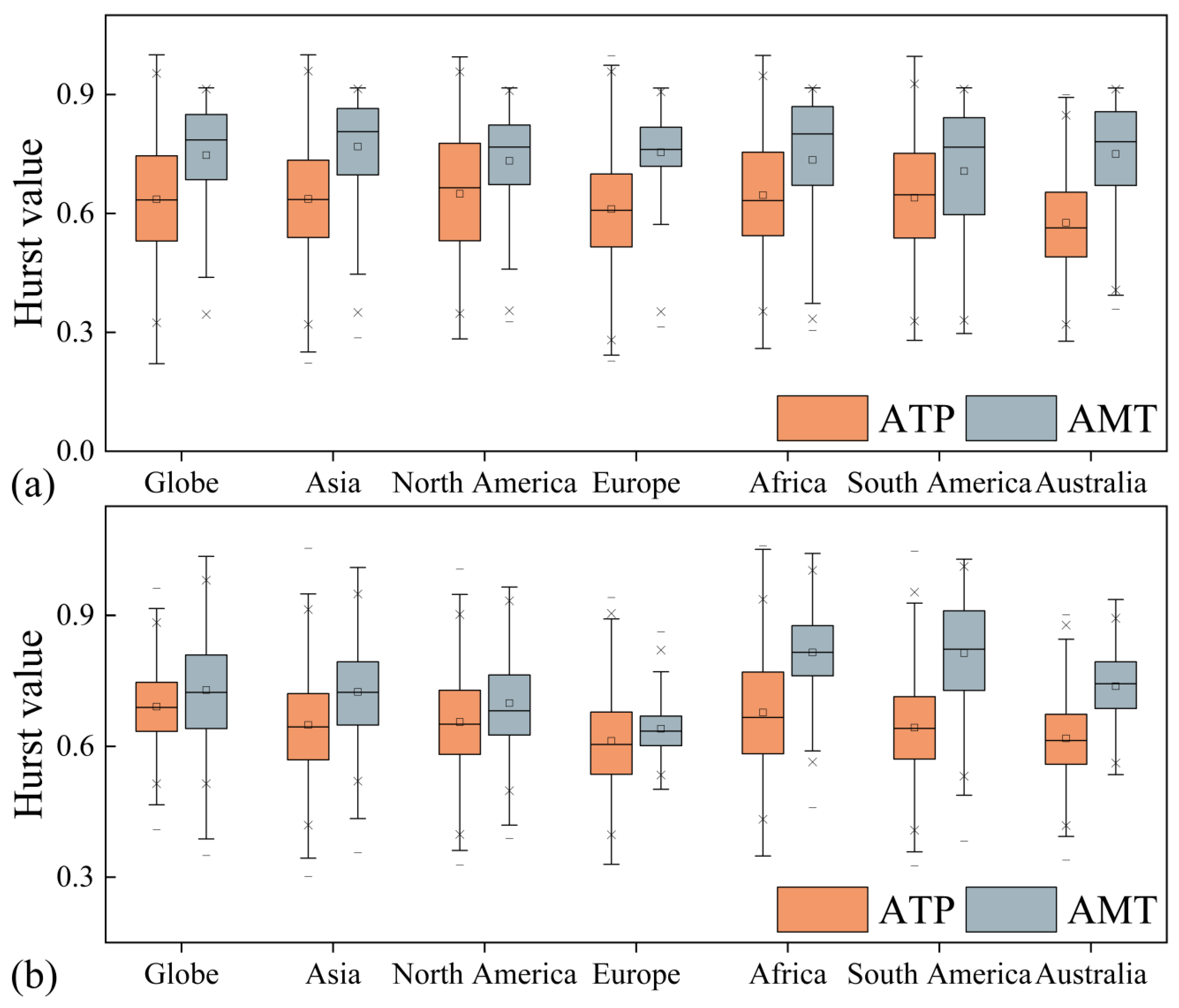
Figure 4 presents box plots of H values for ATP and AMT across global and continental grid points, calculated using different methods. As shown in Figure 4a, based on the WMLE–EMD-DFA method, the median H values for ATP and AMT across all global grid points are 0.63 and 0.86, respectively. Among the six continents, the median H values for ATP are consistently around 0.6, while those for AMT are approximately 0.83. Notably, within each region, the median H value of AMT is always higher than that of ATP. Figure 4b presents box plots of H values for ATP and AMT across global and continental grid points based on the R/S analysis. The results further confirm that, within the same region, the mean and median H values of ATP are consistently lower than those of AMT.
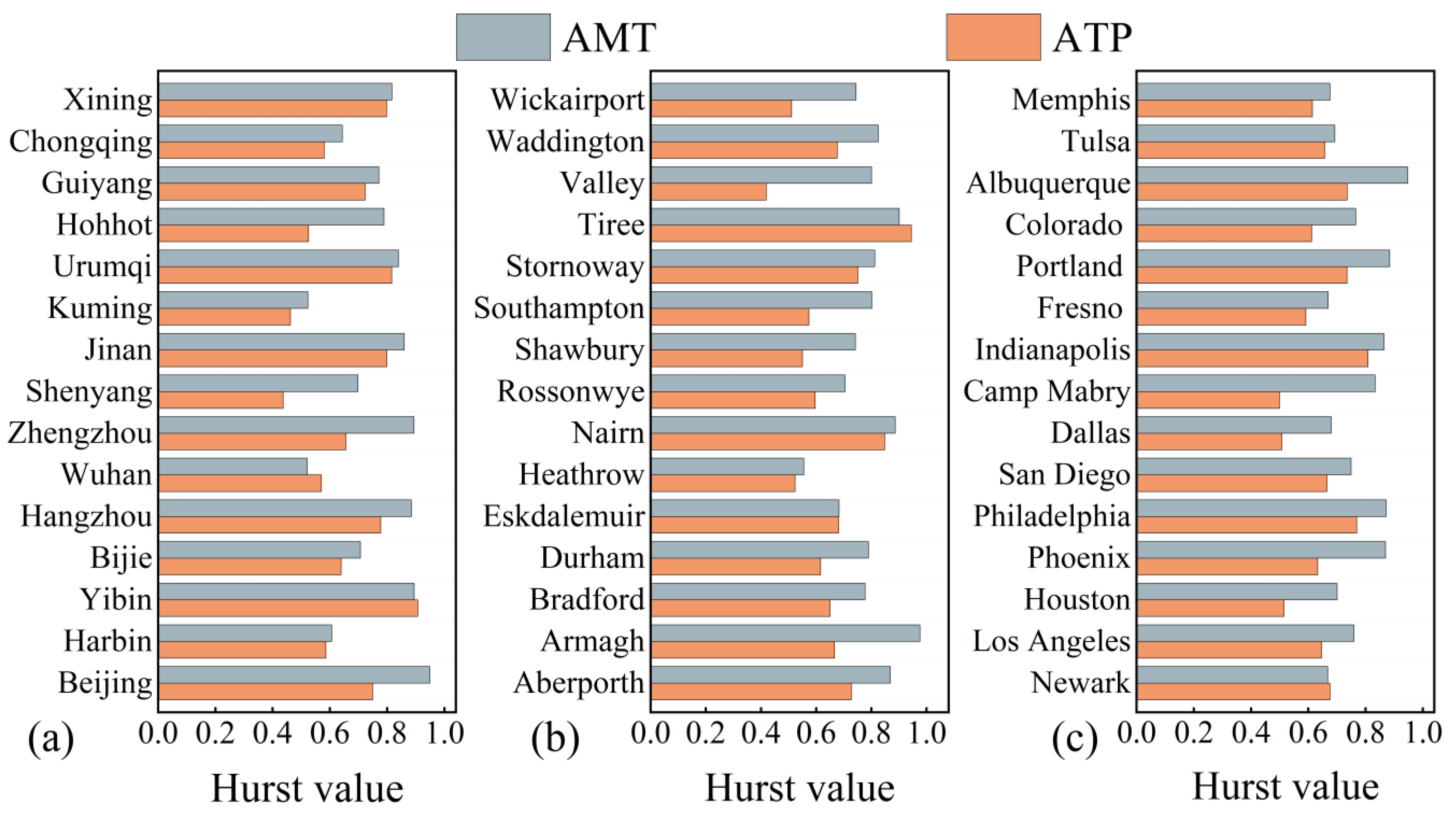
To further verify the robustness of this conclusion, we selected 45 meteorological stations with long-term precipitation and temperature records from China, the U.K., and the U.S. As shown in Figure 5a–c, we computed the H values for ATP and AMT at these stations based on the WMLE–EMD-DFA method to examine their relationships within the same regions. Across all stations, AMT generally exhibits strong LTP, with H values typically exceeding 0.7. In contrast, ATP shows lower H values, usually below 0.7, with some stations even having H < 0.5. Only three stations—Wuhan, Kunming, and Heathrow—have AMT H values below 0.6, and notably, their ATP H values also remain below 0.6. Additionally, at Yibin, Wuhan, Tiree, and Newark, ATP H values slightly exceed those of AMT. However, for all other stations, AMT consistently exhibits higher H values than ATP.
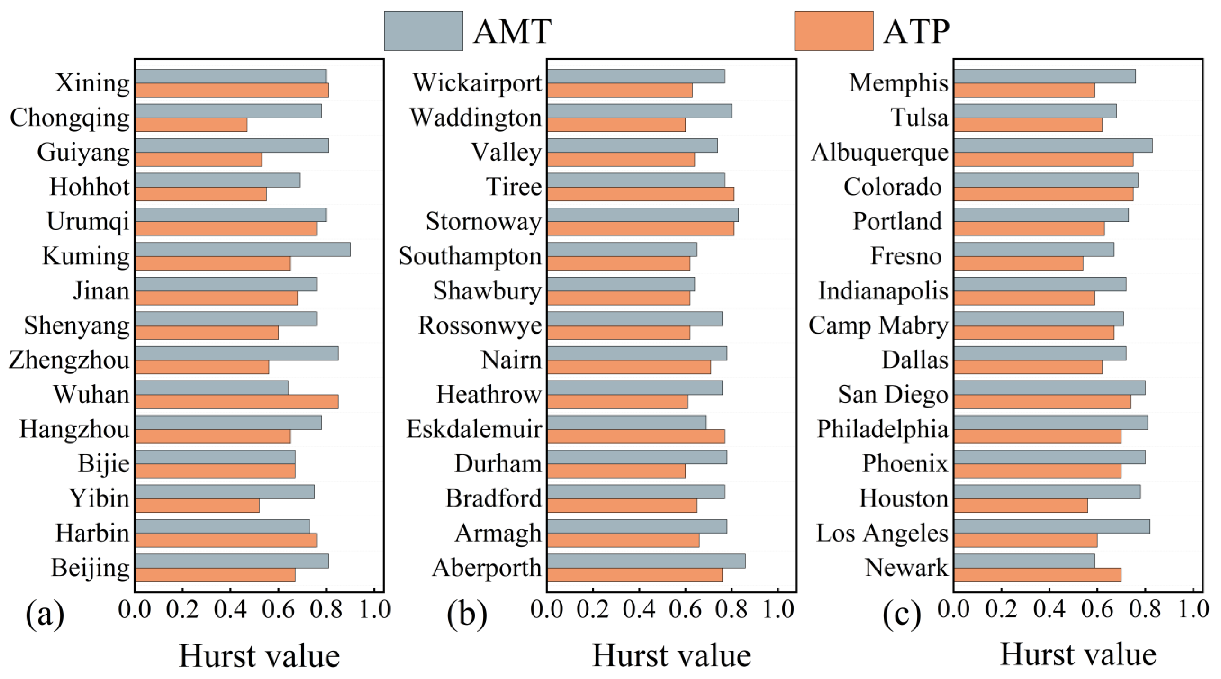
A similar conclusion can also be drawn from Figure 6a–c, where the results are obtained through R/S analysis. For ATP, five Chinese stations have H values below 0.6, while four exceed 0.7. In the U.K., the H values for ATP are more consistent, with all stations above 0.6 and five above 0.7. In the U.S., all H values for ATP are above 0.5, with six stations exceeding 0.7, though none surpass 0.8. In comparison, the H values for AMT are generally higher across all the stations: in China, all 12 stations have H values above 0.7. Similarly, the U.K. stations exhibit higher H values, with 12 stations above 0.7. The U.S. stations show slightly lower H values, with five exceeding 0.7. Across all 45 stations, only seven exhibit higher H values for ATP than those for AMT, with differences generally minimal, averaging 0.07.
Results from the R/S analysis method are presented as supplementary evidence to enhance the robustness of our conclusions. However, since this method has been shown to introduce bias when estimating the H values of time series, our analysis primarily relies on the results obtained from the use of the MLE method. The above results suggest that regardless of whether the analysis is based on gridded or station data, and whether the H values are estimated using the WMLE–EMD-DFA or R/S methods, AMT consistently exhibits higher H values than ATP. Meanwhile, the same conclusion was reached for different spatial scales and data types, further reinforcing the reliability of the findings.

3.2. Spatial Scale Dependence of the Strength of the Hurst Phenomenon

To investigate whether the Hurst phenomenon of ATP and AMT exhibits spatial scale dependency, we resampled the ATP and AMT gridded data over the globe with an original resolution of 0.5° × 0.5° to generate cell-averaged datasets at four coarser resolutions: 2.5° × 2.5°, 5° × 5°, 7.5° × 7.5°, and 10° × 10°. Subsequently, we calculated the H values of cell-averaged ATP and AMT series for all the cells generated under all the four additional resolutions and visualized the results using boxplots, comparing them also with the H values of the globally averaged ATP and AMT series. As shown in Figure S1, the H values increase progressively with the expansion of the spatial-averaging scales, starting from the 0.5° × 0.5° grid resolution. This upward trend is particularly pronounced in the transition from the 10° × 10° grid resolution to the global average. Furthermore, the H values of the globally averaged ATP and AMT series are significantly higher than the median H values of the cell-averaged series at any other resolutions. Similarly, as shown in Figure S2, the results obtained from the R/S analysis also support the same conclusion. These results indicate that the H values of ATP and AMT exhibit a notable upward trend with increasing spatial-averaging scale.
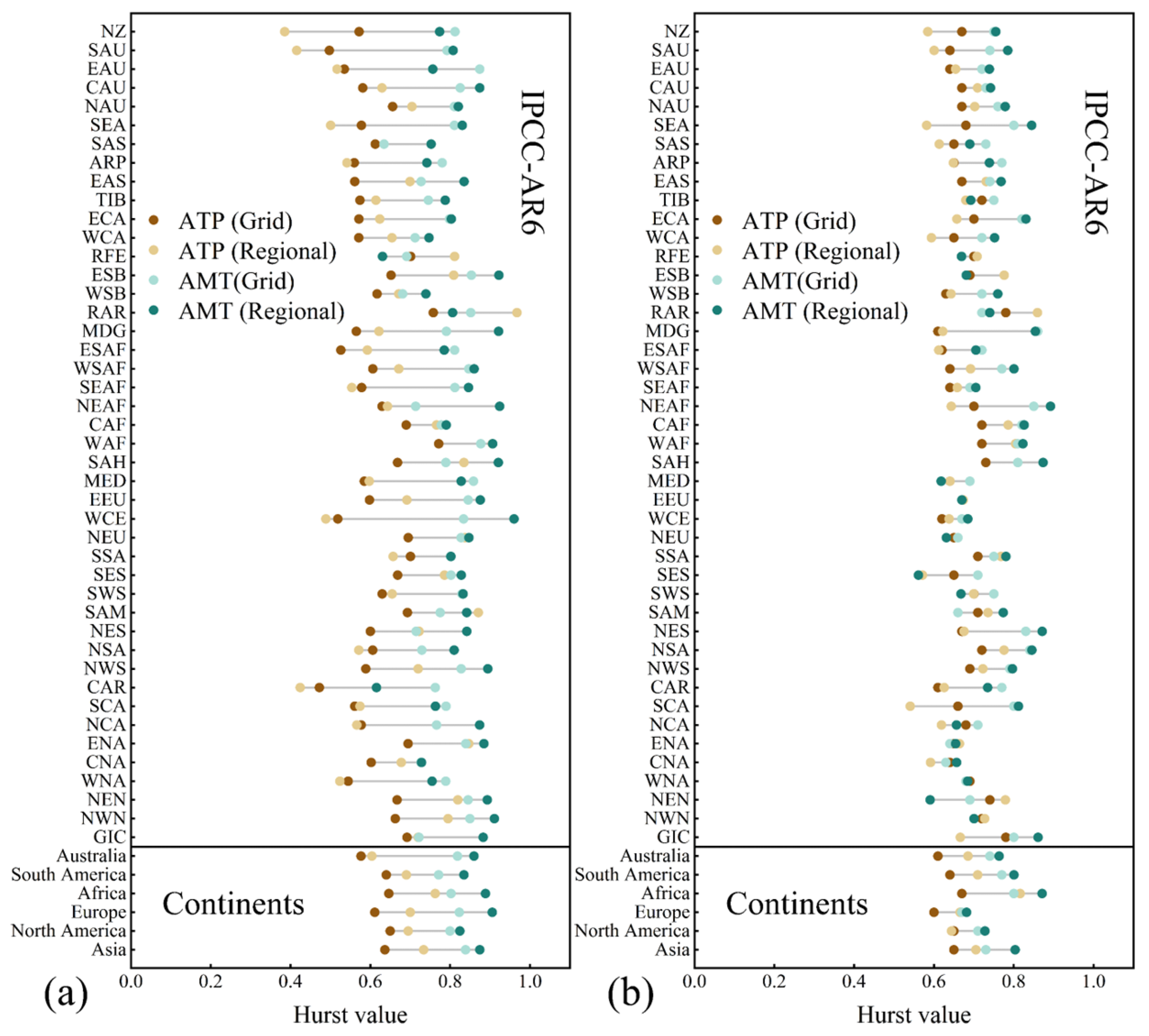
We also calculated the spatially averaged ATP and AMT series for the 44 subregions and six continents and then determined the H values of these spatially averaged ATP and AMT series. Figure 7a shows the H values of the regionally averaged ATP and AMT series together with the middle H values of the grid-point ATP and AMT series within the same region. As shown in Figure 7a, at the continental scale, the H values for continentally averaged ATP and AMT series are significantly higher than the median H values of the grid ATP and AMT series within the same continent, demonstrating further the spatial scale dependence of ATP and AMT. At the subregional scale, Figure 7a illustrates that in nearly all the 41 IPCC-AR6 subregions, the H values of regionally averaged ATP series exceed 0.5, with 16 subregions surpassing 0.7 and 14 falling below 0.6. Similarly, the H values of the regionally averaged AMT series are generally higher, exceeding 0.7 in almost all subregions, except for two where it remains below 0.7. In 32 subregions, the H values of the regionally averaged ATP series are greater than the median H values of grid-point ATP within the same regions, while for AMT, this pattern is observed in 34 subregions (Figure 7a). Additionally, in all 41 subregions, the H values of the regionally averaged AMT are consistently higher than those of the regionally averaged ATP, reinforcing the conclusion that stronger persistence exists in AMT series as compared to ATP series (Figure 7a).
As shown in Figure 7b, the results obtained using the R/S analysis method further confirm the aforementioned conclusion that the LTP of ATP and AMT exhibits spatial scale dependence. Specifically, at the continental scale, the H values of the continentally averaged ATP and AMT series are significantly higher than the median H values of the grid-point ATP and AMT series within the same continent. Among the 44 IPCC-AR6 subregions, 29 subregions show that the H value of the regionally averaged ATP exceeds the median H value of the grid-point ATP, while 32 subregions exhibit a similar pattern for AMT. Moreover, the H values of the regionally averaged AMT are generally higher than those of regionally averaged ATP. This further reinforces the conclusion reached in Section 3.1 that LTP is stronger in AMT than in ATP.

3.3. CDMs of ATP and AMT Averaged at Different Spatial Scales

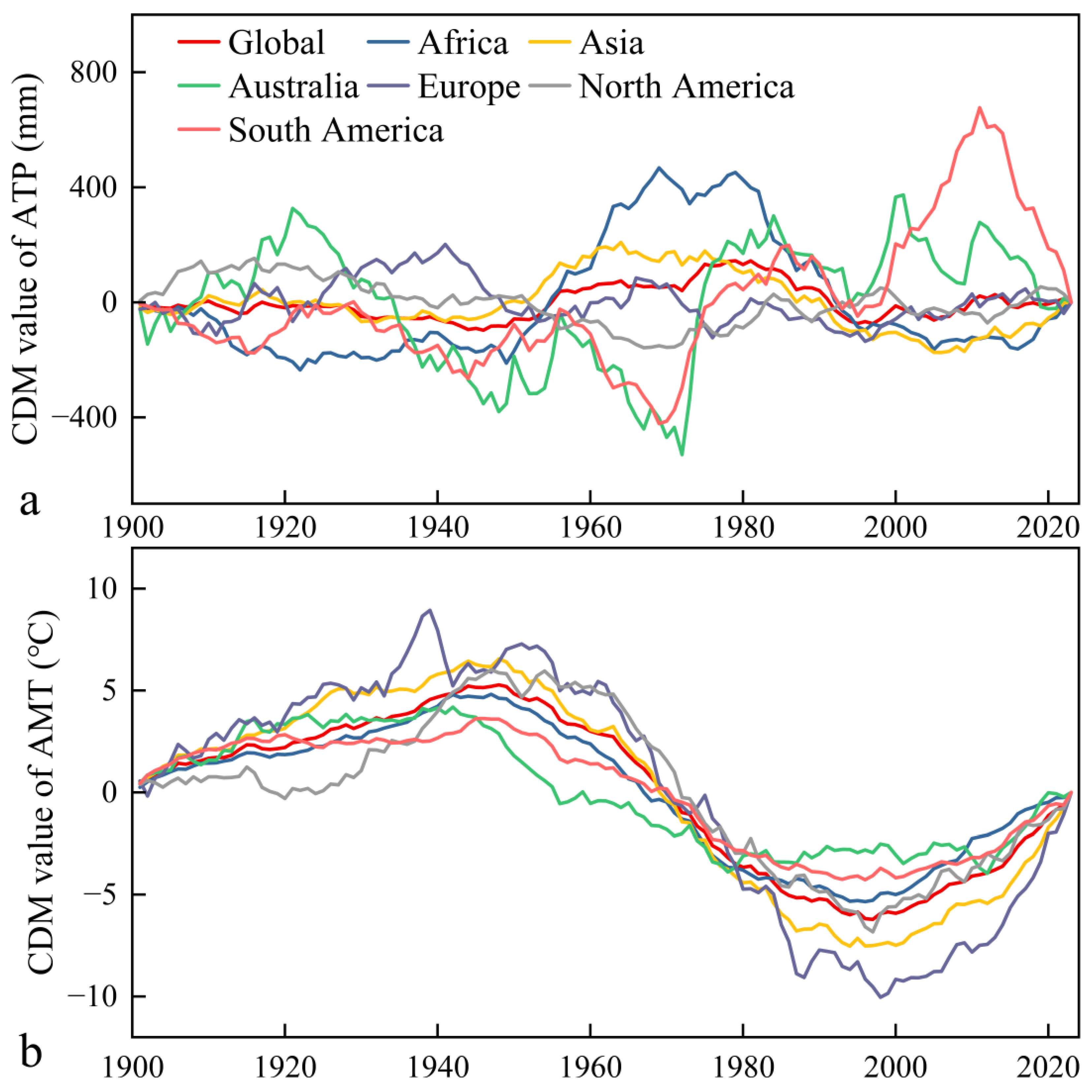
Within individual subregions, the H values of AMT are generally higher than those of ATP, and this phenomenon becomes more pronounced at larger spatial scales. We investigated further the Hurst phenomenon in ATP and AMT by plotting the CDMs of regionally averaged ATP and AMT series. To eliminate the interference caused by the linear trends in regionally averaged AMT and ATP series, we plotted CDM plots (shown in Figure 8) after removing linear trends. Figure 8 presents the CDM time series for the continentally and globally averaged ATP and AMT series. The ATP CDM series exhibit significant differences between continents, with opposing CDM fluctuations in various regions offsetting each other, resulting in a relatively low H value for the globally averaged ATP series. In contrast, the CDM time series for AMT demonstrates a much more consistent pattern across different continents, leading to a higher H value for the globally averaged AMT. Additionally, within the same region, ATP’s CDM time series fluctuates more within the period of observation than AMT’s. The APT’s CDMs’ more frequent fluctuations may due to the fact that ATP is more susceptible to local climate conditions than AMT. The increased sensitivity of ATP to local conditions may obscure its LTP pattern and make the Hurst phenomenon appear weaker in ATP.
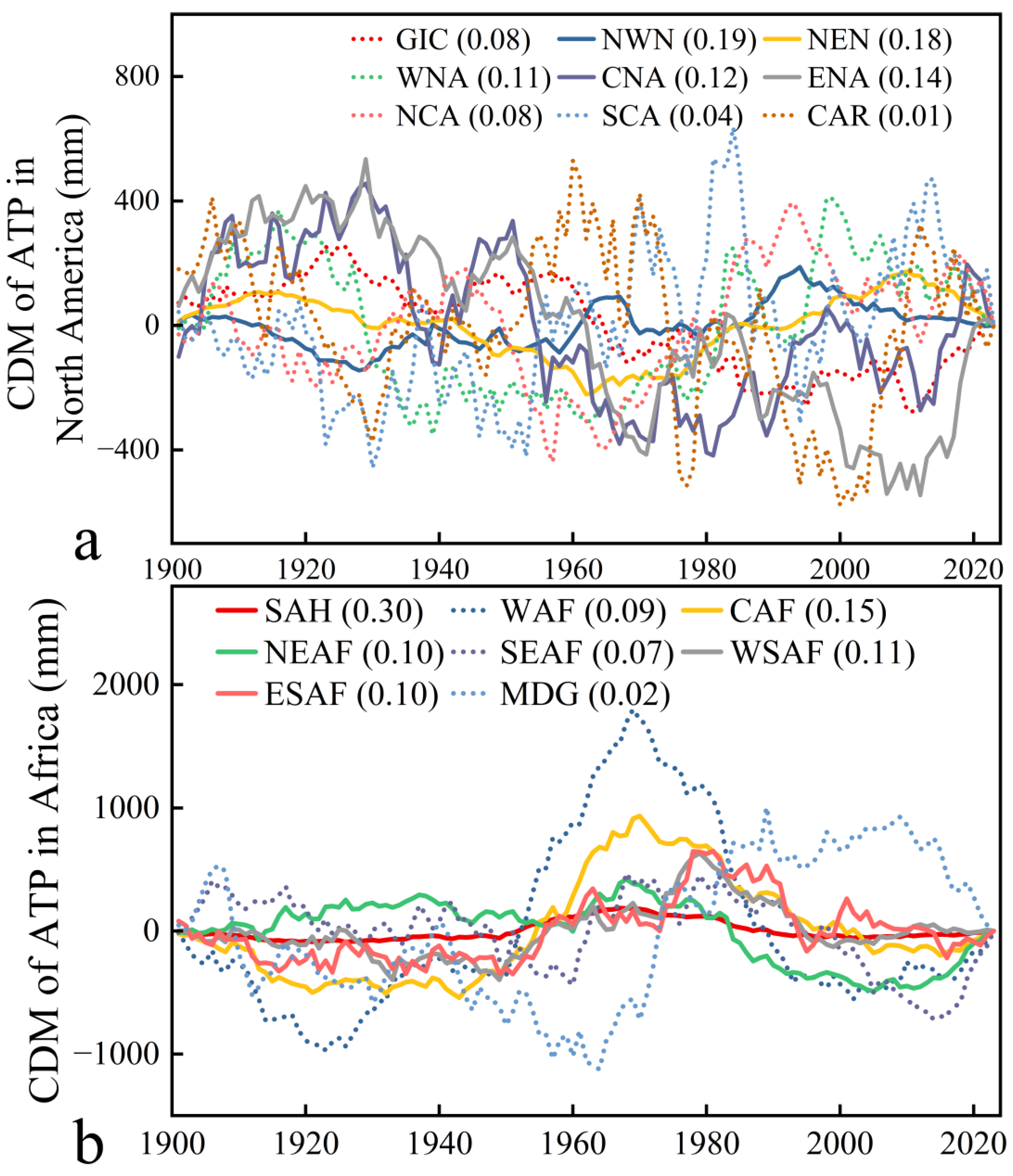
In addition, to better understand the impact of variations in smaller subarea’s ATP’s CDM behaviors on the H values of the APT series obtained by averaging over larger areas, we conducted a detailed analysis using North America and Africa as examples. Figure 9a shows the CDM series of the regional-average ATP for subregions within North America, revealing strong fluctuations and distinct patterns across different subregions. Multiple linear regression analysis indicates that the NWM, NEN, CAN, and ENA subregions have the most significant impact on the regional-average ATP in North America. The substantial differences in the CDM behaviors among these subregions contributed to the relatively low H value for North America’s regional-average ATP.
Figure 9b displays the regionally averaged ATP’s CDM behaviors of all the subregions in Africa, where the SAH subregion’s influence on Africa’s regional average ATP is significantly higher than those of all the other subregions. Additionally, subregions with CDM behavior similar to SAH, such as CAF, WSAF, NEAF, and ESAF, tend to have relatively larger regression coefficients as well. The similarity in the CDM behaviors among these subregions contributed to relatively high H value for Africa’s regional-average ATP. This additional analysis demonstrated that, unlike AMT, even for nearby subregions, the regionally averaged ATP’s CDM behaviors may be very different from each other, and this difference contributed to the low H values for some continents or larger areas.

3.4. Similarities in the CDMs of AMT and ATP Averaged at Different Spatial Scales

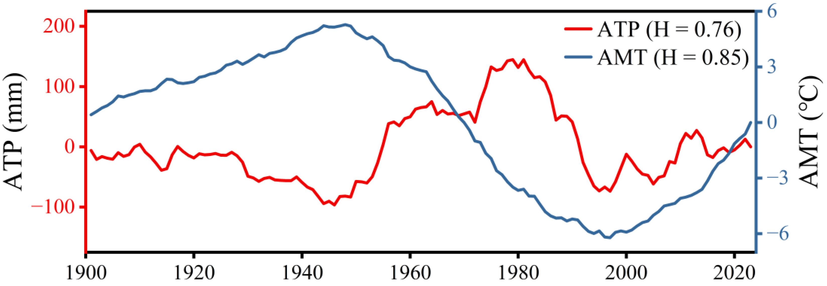
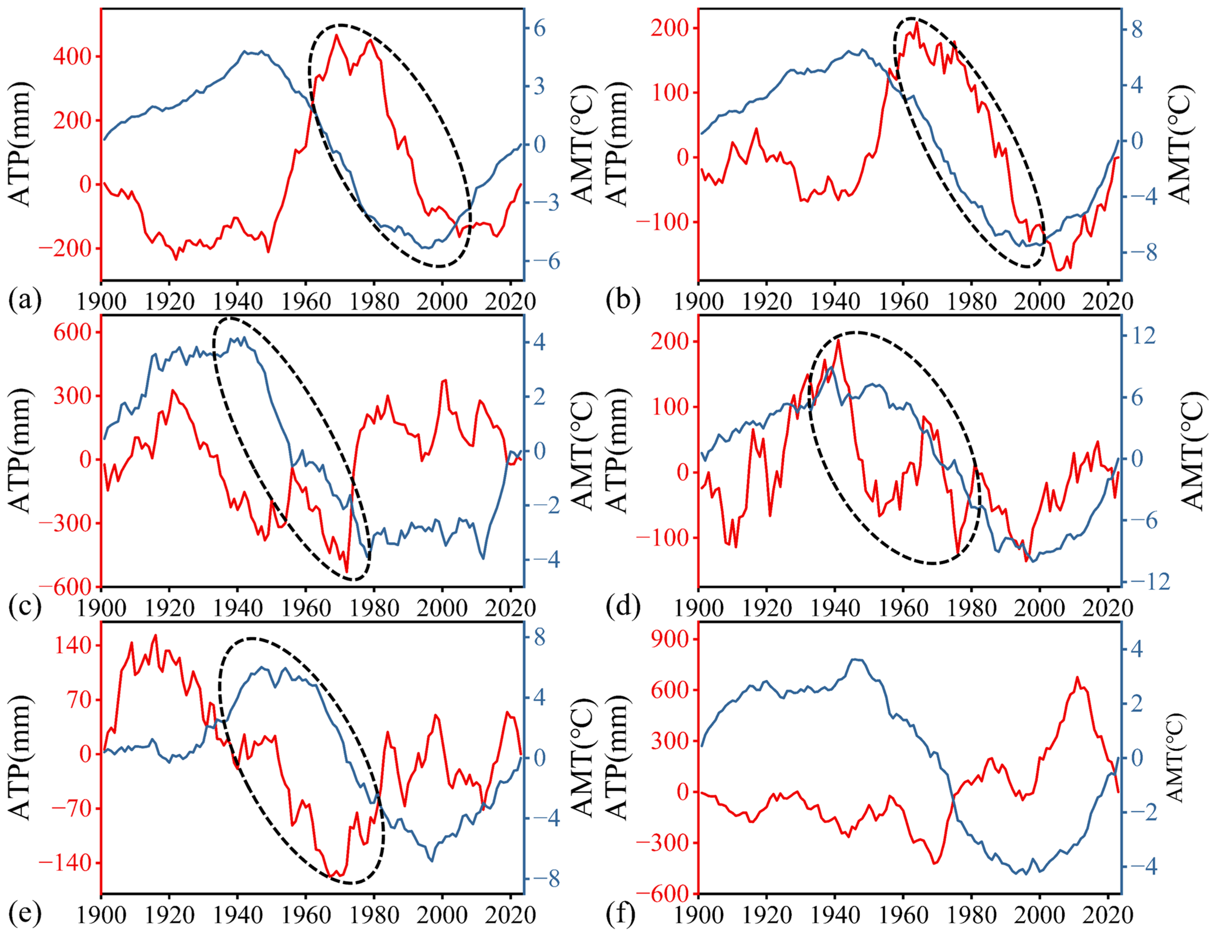
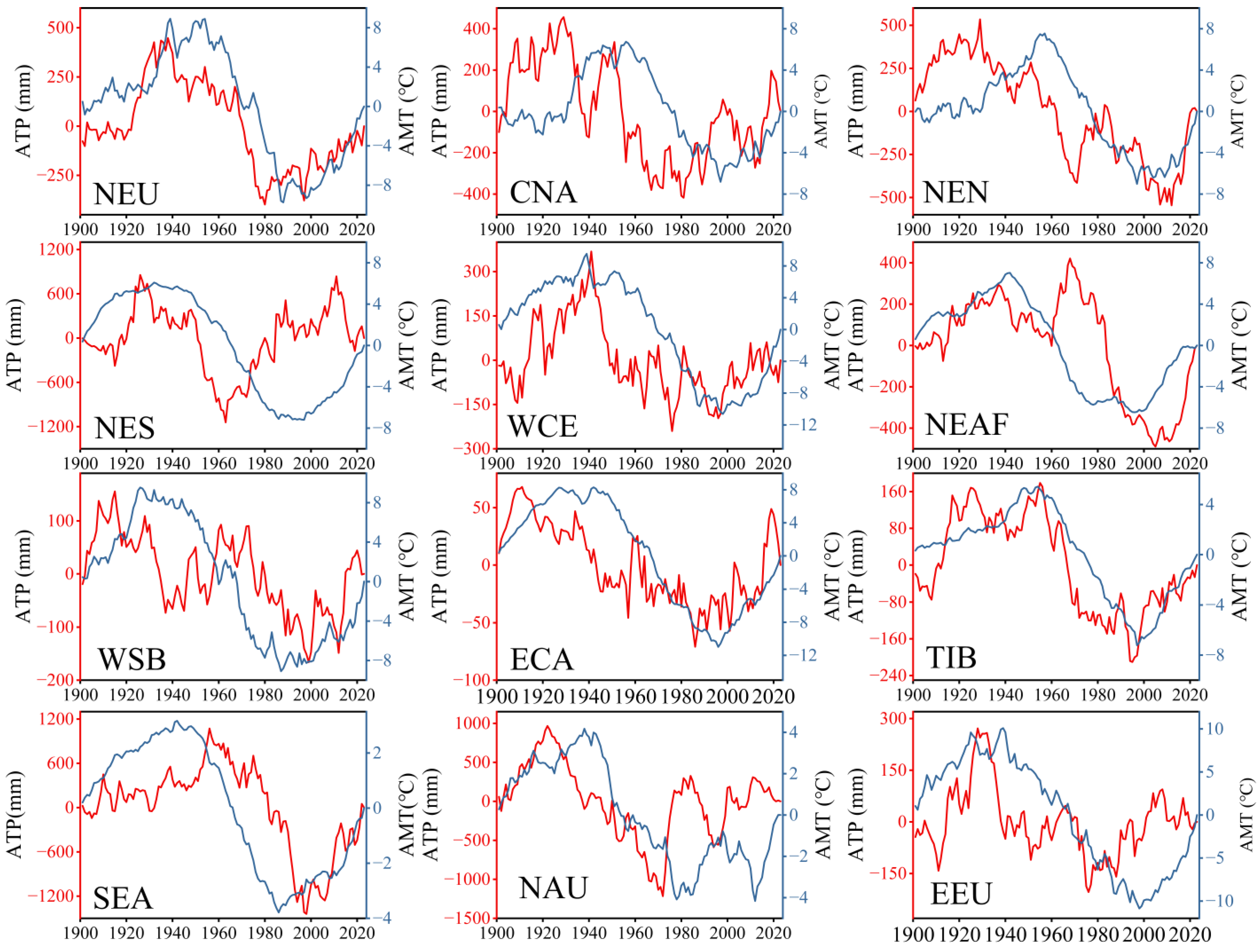
In Figure 10 and Figure 11, we plotted the CDM series of ATP and AMT for the globe and six continents on a dual y-axis graph, revealing some interesting observations: in Asia, Australia, Europe, and South America, the CDM graphs for the regionally averaged ATP and AMT series exhibit some similar patterns. In Europe, in particular, the CDMs of ATP and AMT display nearly identical overall trends across all time periods, suggesting that the Hurst phenomenon in ATP may be caused by or at least influenced by that of the AMT. However, as shown in Figure 10 and Figure 11, due to the complex climatic interactions over large spatial scales, the similarities in CDM patterns of ATP and AMT averaged over continents and the globe are not obvious. That is why we further analyzed the CDM behaviors of ATP and AMT averaged at smaller spatial scales. Among the 44 subregions defined in IPCC-AR6, over half show similar CDM behaviors between regional-averages of ATP and AMT, with 12 subregions exhibiting high consistency throughout the observation period (see Figure 12). Additionally, an analysis of the CDM time series for ATP and AMT from 45 observation stations in China, the United Kingdom, and the United States shows even stronger similarity in CDM behavior. Figure 13 displays the CDM time series for ATP and AMT at 12 of these stations, where the ATP and AMT CDM time series for Aberporth, Rosehearty, and Phoenix are nearly identical.
We also found that the Hurst phenomenon in ATP is not necessarily influenced solely by the local AMT; it may also be affected by the AMT over a larger area. The influence of regionally averaged AMT over a larger area on a locally averaged ATP may be revealed by gradually combining the AMT over larger and larger areas surrounding the area over which the ATP is averaged. We only attempted to analyze the similarities between the CDM time series of regional-average ATP in several areas and their corresponding regional-average AMT over larger areas. As shown in Figure 14, the CDM behavior of regional-average ATP in Africa’s GIC region is not similar to that of its own regional-average AMT, but it resembles the CDM behavior of the AMT averaged over Africa entirely. Similarly, the CDM behavior of the regional-average ATP in the CAU region of Australia is more similar to the CDM behavior of the regional-average AMT for entire Australia than to that of the regional-average AMT over the CAU region.
Furthermore, we conducted Granger causality tests between ATP and AMT for the 12 IPCC-AR6 subregions and the 12 meteorological stations where similarity in CDMs was identified; the results are presented in Table 1. Table 1 shows that the optimal lag orders for the impact of AMT on ATP do not exceed 3 in most regions and stations. Table 1 also shows that, in 9 out of the 12 IPCC-AR6 subregions and 7 out of the 12 meteorological stations, AMT is the Granger cause of ATP with p-values less than 0.05. In some meteorological stations, AMT was not identified as the Granger cause of ATP, which may partly be a result of the relatively short time series. Observation records in stations across China and the United States generally do not exceed 100 years, which may have influenced the Granger causality test results. Nevertheless, confirmation of the Granger causality in more than half of the subregions and stations led us to hypothesize that the Hurst phenomenon in AMT is at least one of the causes of the Hurst phenomenon in ATP.

4. Discussion

4.1. Factors Affecting the Hurst Exponents of the Regionally Averaged ATP and AMT Series

The Hurst phenomenon is closely associated with high uncertainty and LTP [13,85]. Analyzing the Hurst phenomenon in ATP and AMT is crucial for understanding the long-term changes and behavioral patterns within the climate system. In their analysis of the Hurst phenomenon in ATP, O’Connell et al. mathematically proved that when multiple independent time series with different Hurst exponents are combined, the Hurst exponent of the overall process tends to align with that of the series with the highest H value, thereby making the LTP primarily driven by the process with the highest H value. This is verified in our study using AMT series [12]. For example, the regionally averaged AMT H value for Africa is 0.89, which is close to the highest H value in the subregions of Africa, i.e., NEAF (0.92). Similarly, the regionally averaged AMT H value for Asia is 0.87, which is also close to the highest H value in the subregions of Asia, i.e., SEA (0.84). We speculate that other GTS may also exhibit similar spatial-averaging characteristics.
An important finding of this study is that noticeable differences in the CDM plots of the ATP series exist across almost all regions, whereas the CDM plots of AMT series appear relatively similar and stable across almost all regions. Consequently, the H value of ATP is generally lower than that of the AMT of the same region. This observation aligns with findings from multiple studies indicating that the H value of precipitation tends to be lower, with the mean and median of the H values of grid precipitation data all over the world ranging from 0.6 to 0.7 [6,13,41]. Our analysis reveals further that, on a larger spatial scale, the H value of regionally averaged ATP is significantly lower than that of regionally averaged AMT.
By examining the CDM plots of regionally averaged ATP across different continents, we found that the low H value of globally averaged ATP may result from the opposing fluctuations in the regionally averaged ATP’s CDMs of each continent (Figure 8a). This conclusion is also supported by the study of [6]. The CDM fluctuation patterns also help to explain the relatively high H value of the globally averaged AMT, as the CDMs of regionally averaged AMT across different continents have a very similar fluctuation pattern (Figure 8b). Additionally, by analyzing the CDM fluctuation patterns across different regions and applying stepwise regression, we further elucidated the causes of the low H value of continentally averaged ATP in North America and the high H value of continentally averaged ATP in Africa (Figure 9).

4.2. Possible Causes of Hurst Phenomenon

As shown in Section 3.3, unlike AMT, significant regional differences in the CDMs of ATP make it impossible for the similarity between the CDM plots of AMT and ATP to exist everywhere or at all the spatial scales of averaging. The fact that there are still a large number of subregions and ground observation points where the CDM plots of ATP and AMT fluctuate very similarly with each other may be viewed as evidence supporting our hypothesis that it is the LTP in AMT that causes or at least partly causes the LTP in ATP.
O’Connell et al. found in their study that the CDM fluctuation patterns of annual precipitation and annual runoff in the Nile River are highly similar, leading them to infer that the Hurst phenomenon in runoff may originate from precipitation [6]. In our study, we also arrived at an interesting conclusion: in many regions, the CDMs of ATP and AMT exhibit similar fluctuation patterns. Furthermore, as discussed in Section 3.3 and Section 3.4, we found that CDM fluctuation patterns are closely related to the Hurst values. For instance, if multiple subregions within a larger region exhibit highly similar CDM fluctuation patterns, their Hurst values tend to be higher, indicating a more pronounced Hurst phenomenon. This finding prompted us to investigate further the origin of the Hurst phenomenon in ATP. Our additional analysis revealed that AMT is the Granger cause of ATP fluctuations in 9 out of the 12 IPCC-AR6 subregions and 7 out of the 12 meteorological stations where the CDMs of AMT and ATP fluctuate similarly. The similarities in the CDMs of ATP and AMT occurring at so many subregions and stations are unlikely to be coincidental. Furthermore, in subregions and stations where similar CDM behaviors were observed, most of them also have the AMT series that is the Granger cause of the ATP series. This additional evidence supports further our hypothesis that the Hurst phenomenon in AMT may drive the Hurst phenomenon in ATP or that both are influenced by a common driving factor.
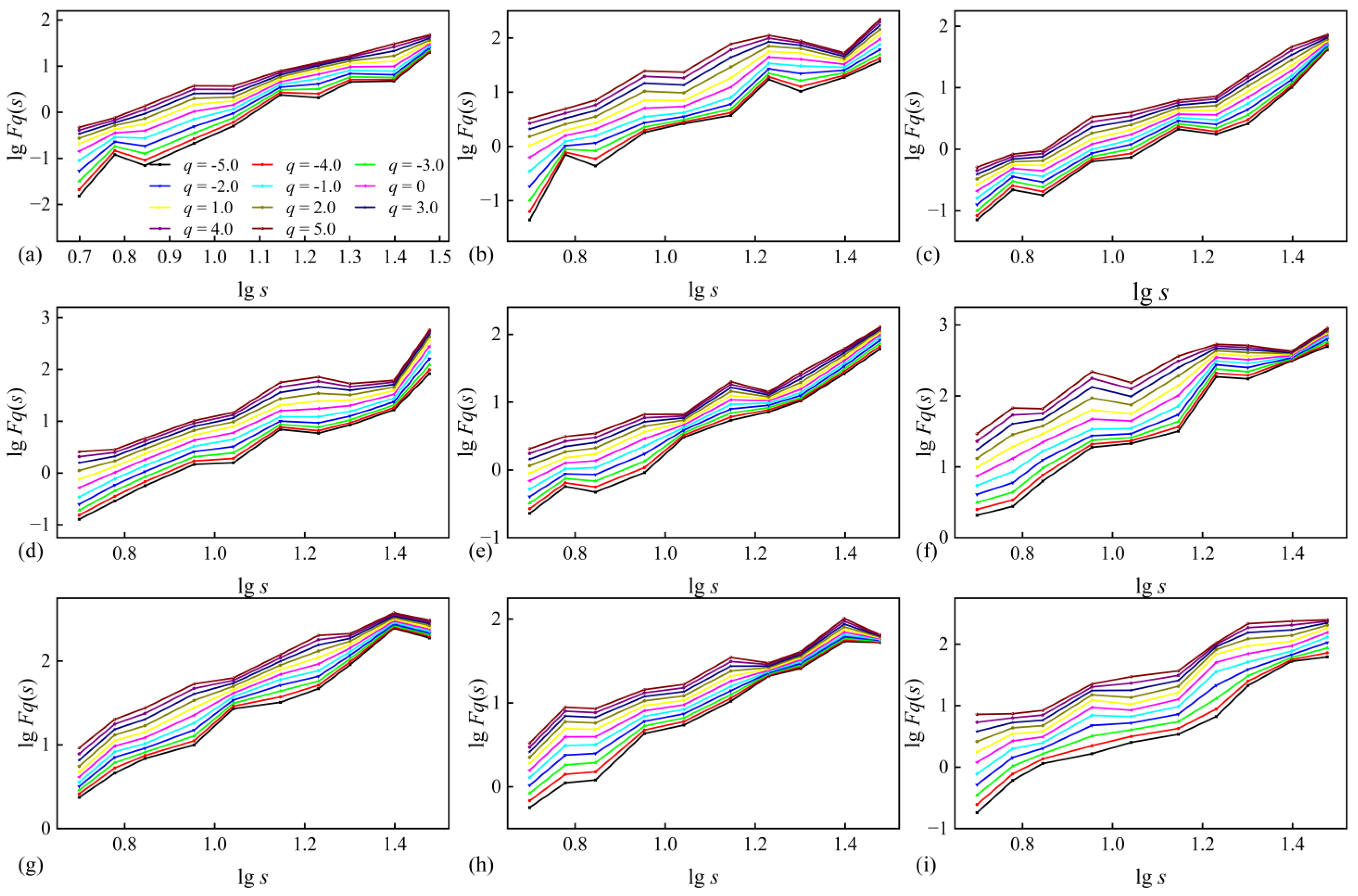
Due to the substantial variability in local climate patterns and complex surface conditions of the ground, it is often challenging to reliably identify the intrinsic relationship between precipitation and temperature at small spatial scales. To reduce the interference of local noises and uncover possible coupling structures, we applied MF-DCCA at global and continental scales. MF-DCCA allows us to examine the multifractal nature and long-range cross-correlations between ATP and AMT series. The results are presented in Figure 15 and Figure 16. Figure 15 presents the log–log plots of the fluctuation function Fq(s) versus segment length or time scale s for a series of moment orders q ∈ [−5, 5], derived from both global and continental ATP and AMT series. Across all continents and the globe, the fluctuation functions exhibit approximate linearity in the log–log space, indicating that the cross-correlations between ATP and AMT do follow power-law scaling relationships. This validates the use of the generalized cross-correlation exponent H(q) to describe their long-range dependence and multifractal coupling structure. Figure 16 shows the variations in the estimated H(q) versus q for different continents and the globe. At the global scale, H(q) decreases from 1.076 at q = −5 to 0.756 at q = 5, with a central value of 0.849 at q = 0, suggesting persistent and memory-driven coupling between ATP and AMT. As shown in Figure 16, all regions exhibit a decreasing trend in H(q) as q increases, indicating the presence of multifractality. However, the strength and shape of the H(q) curves vary significantly across different regions. Australia, South America, and the Southern Hemisphere display more pronounced multifractal behavior, characterized by lower H(q) values and steeper, more curved profiles, suggesting weaker correlations and greater sensitivity to fluctuation magnitude. In contrast, Africa, Europe, and the Northern Hemisphere exhibit weaker multifractality, with flatter and nearly linear H(q) curves, indicative of more homogeneous scaling.
The MF-DCCA results collectively demonstrate that the Hurst phenomenon observed in ATP may be closely associated with that of AMT, and that their multifractal coupling structure exhibits significant spatial heterogeneity. Stronger persistence in some regions may be driven by more stable climatic regimes or enhanced land–atmosphere feedbacks, while weaker or more scale-sensitive coupling in others may reflect greater climate variability or differing teleconnection influences. Overall, these findings underscore the importance of regional-scale analysis in understanding the complex and long-memory nature of hydroclimatic interactions.
Furthermore, since the water vapor content in the atmosphere is the principal driver of precipitation [63,64] and temperature has a significant effect on it [65], any small changes in AMT may result in some or significant changes in ATP. Thus, physically, the Hurst phenomenon in AMT is likely to be one of the causes of the Hurst phenomenon in ATP. The observed statistical linkage between the LTP of AMT and ATP may be attributed to several interacting physical processes. Elevated temperatures enhance evaporation and increase the atmosphere’s capacity to hold moisture, intensifying the hydrological cycle and creating conditions conducive to prolonged or extreme precipitation events [86]. This thermodynamic effect, governed by the Clausius–Clapeyron relationship, has been shown to increase extreme precipitation intensity at rates of approximately 6–7% per degree Celsius of warming, particularly in convective systems [87,88]. In addition to the thermodynamic influence, temperature variations can modulate precipitation characteristics through their impact on large-scale atmospheric circulations. Shifts in monsoonal strength, mid-latitude westerlies, and subtropical highs, often induced by warming, alter moisture transport and convergence patterns [89,90]. These dynamic changes contribute to spatially and temporally persistent anomalies in precipitation, thereby reinforcing the memory structures in ATP. Land–atmosphere feedbacks further amplify these effects. Soil moisture deficits associated with warming can suppress evapotranspiration and rainfall recycling [91], while positive feedbacks from latent heat release during heavy precipitation events can sustain atmospheric instability over extended periods [92]. These feedbacks are particularly relevant in regions prone to compound extremes, where persistent hot-dry or wet-warm conditions may co-evolve, enhancing LTP in both temperature and precipitation fields [93]. Together, these mechanisms provide a physically consistent interpretation of the observed LTP propagation from AMT to ATP. They underscore the importance of integrating climatic feedbacks, moisture availability, and circulation variability when interpreting persistence in hydroclimatic time series, particularly under future climate conditions. Thus, physically, the Hurst phenomenon in AMT is likely to be one of the causes of the Hurst phenomenon in ATP.

4.3. Hurst Exponent Estimations and Data Limitation

Selecting an appropriate method is crucial for accurately estimating the H values in time series. To achieve the most precise evaluation of the H values for ATP and AMT series, this study employs the WMLE–EMD-DFA method. Additionally, the R/S analysis method, as one of the earliest and most widely used tools for estimating H values, remains valuable in practical applications and is still one of the most commonly used methods for H value assessment in hydrological studies [19]. Therefore, despite existing research indicating that the R/S method may have certain biases in estimating H values, we still reported the results obtained using this method. It is important to emphasize that our research conclusions are primarily based on the WMLE–EMD-DFA method and that the results obtained using the R/S analysis method serve only as a reference and comparison. Although the exact values derived from the R/S and WMLE–EMD-DFA methods exhibit slight differences [73], they led to similar conclusions: compared to ATP, AMT at the same grid point or region has a higher H value, indicating a stronger LTP; furthermore, similar to ATP, the H values of AMT also demonstrate the effect of spatial aggregation.
In addition to selecting an appropriate method for estimating the Hurst exponent, it is essential to use the longest possible ATP and AMT time series. Although the CRU dataset used in this study provides over 120 years of global climate records and many ground-based stations now provide data more than 100 years long, the availability of even longer observational datasets remains limited. As an illustrative case, we conducted a sensitivity analysis using globally averaged ATP and AMT series from the CRU to examine how time series length affects statistical inferences. The results, summarized in Table S1, show that the causal relationship from temperature to precipitation remains statistically significant when the time series spans at least 60–70 years, but becomes insignificant when the time series are reduced to 50 years. This indicates that insufficient data length may compromise the reliability of causality detection. The evaluation of long-range dependence—such as the Hurst phenomenon—may also be influenced by time series length. Extending climate records, where possible, can substantially improve the robustness and credibility of persistence analysis.

5. Conclusions

Using gridded annual precipitation data from regions distributed across the globe, the recent studies of [6] demonstrated for the first time that the H values of ATP increase with the spatial scale of averaging and provided evidence, confirming that the LTP in annual river flows are attributable to the LTP in basin average precipitation. Using a different set of gridded precipitation data (the one we used is the CRU’s precipitation dataset from 1901 to 2023, while [6] used the GPCC dataset from 1901 to 2013) for regions all across the globe and different estimation methods for the Hurst exponent (we used both the maximum likelihood and the detrended fluctuation analysis methods while the one used by [6] is the aggregated variance method which is also referred to as the climacogram method), we confirmed their finding that the H values of ATP increase with the spatial scale of averaging. Our study also examined the Hurst phenomenon of AMT on a global scale, with a particular focus on the potential influence of the Hurst phenomenon in AMT on that of ATP. The main findings are summarized as follows.
  • Across various spatial scales globally, the H values of AMT are generally higher than those of ATP, particularly with larger spatial scales of averaging. This finding is consistently validated using both gridded data covering all the land surfaces of the globe and 45 individual ground station datasets.
  • Similarly to ATP, the H values of AMT also increase with the spatial scale of averaging. For all continents, the H values for continentally averaged ATP and AMT series are significantly higher than the median of the H values of grid-scale ATP and AMT series. In the 44 subregions defined by the IPCC-AR6, the H values of the regionally averaged ATP series exceed their grid-scale median H values in 29 of the subregions, while the H values of the regionally averaged AMT series exceed their respective grid-scale median H values in 32 of the subregions.
  • The CDM time series of regionally averaged AMT follow a similar fluctuation pattern across all areas, but the CDM time series of regionally averaged ATP series do not follow a similar pattern. The difference in the CDM fluctuation patterns of regionally averaged ATP series contributed to the low H values of some continents and larger areas.
  • In 12 of the 44 subregions analyzed, the CDMs of regionally averaged ATP fluctuate very similarly to the way the CDMs of the same regionally averaged AMT fluctuate. At 12 of the 45 ground monitoring stations, the CDMs of the ATP also fluctuate very similarly with the way the CDMs of AMT fluctuate. These similarities are observed throughout the observation period of 1901 to 2023 (see Figure 13 and Figure 14). Moreover, Granger causality tests showed that AMT is the Granger cause of ATP in 9 out of the 12 IPCC-AR6 subregions and 7 out of the 12 meteorological stations where similarities of CDM fluctuations in AMT and ATP were observed. The MF-DCCA analysis results reveal that for all regions at both global and continental scales, the ATP and AMT series are power-law cross-correlated. These findings suggest that the LTP of AMT and ATP are interrelated, implying that the Hurst phenomenon observed in AMT may be a potential driver of the Hurst phenomenon in ATP, or alternatively, that both may stem from a common underlying cause. More in-depth research may be conducted to verify further this new and insightful hypothesis.
Taken together, our results highlight a globally consistent pattern in which temperature exhibits stronger and more persistent memory than precipitation, particularly as spatial averaging increases. This finding may reflect fundamental differences in the long-range dependence structures of atmospheric temperature and moisture processes across climatic regions. The observed cross-scale coherence of AMT and ATP, and the directional causality from AMT to ATP, suggest that global warming-induced changes in temperature variability could have cascading effects on precipitation persistence at regional and global scales.
Building on these insights, future research could further investigate the physical mechanisms linking temperature and precipitation persistence, especially under climate change scenarios. Extending the current analysis to include other climatic variables (e.g., soil moisture, sea surface temperature), or using high-resolution model simulations, may help to disentangle the potential feedbacks and teleconnections involved. Moreover, exploring these relationships in sub-seasonal and seasonal scales would provide a more comprehensive understanding of the temporal dynamics of long-term persistence in the Earth’s climate system.

Supplementary Materials

The following supporting information can be downloaded at https://www.mdpi.com/article/10.3390/fractalfract9060385/s1. Figure S1: Hurst values of ATP and AMT series based on the WMLE–EMD-DFA method obtained by averaging over different spatial scales; Figure S2: Hurst values of ATP and AMT series based on the R/S analysis method obtained by averaging over different spatial scales; Table S1: Granger causality test results under different time series lengths.

Author Contributions

H.Z.: Conceptualization, Methodology, Writing—original draft. Y.G.: Methodology, Review, Funding Acquisition, Supervision. All authors have read and agreed to the published version of the manuscript.

Funding

This research was supported by the Natural Sciences and Engineering Research Council of Canada (NSERC, grant number RGPIN-2023-04832), which also covered the article processing charge (APC).

Data Availability Statement

The CRU time series datasets, produced by the United Kingdom’s National Centre for Atmospheric Science, are used in this study. We employed the CRU’s gridded monthly precipitation and temperature data (https://crudata.uea.ac.uk/cru/data/hrg/, accessed on 1 December 2024). Additionally, precipitation and temperature data from ground meteorological stations in China and the United States were sourced from NOAA (https://www.ncei.noaa.gov/cdo-web/, accessed on 1 December 2024), while data for ground meteorological stations in the United Kingdom were obtained from the UK Meteorological Office (https://www.metoffice.gov.uk/research/climate/maps-and-data/historic-station-data, accessed on 1 December 2024). These websites were accessed on 1 December 2024. For implementing the AR6’s division of regions, we used the “regionmask.defined_regions.ar6.land” function in Python 3.12.0. The specific code for Whittle’s maximum likelihood estimator (WMLE) method and detrended fluctuation analysis (DFA) method is provided by Clément Roume et al. and can be accessed at https://github.com/clementroume/Whittle_maximum_likelihood_estimator_tutorial, accessed on 1 December 2024. In MATLAB (Python version 3.12.0), empirical mode decomposition (EMD) can be implemented using the “emd()” function. For conducting the Granger causality test, the construction of the vector autoregression (VAR) model and the selection of the optimal lag order can be performed using the “VARselect()” function in R. The “grangertest()” function is then used to conduct the Granger causality test.

Acknowledgments

The authors would like to express their sincere gratitude to the Natural Sciences and Engineering Research Council of Canada (NSERC) for its support. The authors also thank the China Scholarship Council (CSC) for supporting Huayu Zhong’s PhD studies at McMaster University. We are especially grateful to the two anonymous reviewers for their constructive comments and valuable suggestions, which greatly improved the quality of this manuscript.

Conflicts of Interest

The authors declare no conflicts of interest relevant to this study. We declare that we have no financial and personal relationships with other people or organizations that can inappropriately influence our work, and there is no professional or other personal interest of any nature or kind in any product, service and/or company that could be construed as influencing the position presented in, or the review of, the manuscript entitled.

References

  1. Hurst, H.E. Methods of Using Long-Term Storage in Reservoirs. Proc. Inst. Civ. Eng. 1956, 5, 519–543. [Google Scholar] [CrossRef]
  2. Hurst, H.E. Long-Term Storage Capacity of Reservoirs. Trans. Am. Soc. Civ. Eng. 1951, 116, 770–799. [Google Scholar] [CrossRef]
  3. Salas, J.D.; Boes, D.C.; Yevjevich, V.; Pegram, G.G.S. Hurst Phenomenon as a Pre-Asymptotic Behavior. J. Hydrol. 1979, 44, 1–15. [Google Scholar] [CrossRef]
  4. Koutsoyiannis, D. Climate Change, the Hurst Phenomenon, and Hydrological Statistics. Hydrol. Sci. J. 2003, 48, 3–24. [Google Scholar] [CrossRef]
  5. O’Connell, P.E.; Koutsoyiannis, D.; Lins, H.F.; Markonis, Y.; Montanari, A.; Cohn, T. The Scientific Legacy of Harold Edwin Hurst (1880–1978). Hydrol. Sci. J. 2016, 61, 1571–1590. [Google Scholar] [CrossRef]
  6. O’Connell, E.; O’Donnell, G.; Koutsoyiannis, D. On the Spatial Scale Dependence of Long-Term Persistence in Global Annual Precipitation Data and the Hurst Phenomenon. Water Resour. Res. 2023, 59, e2022WR033133. [Google Scholar] [CrossRef]
  7. Villa, D.L.; Schostek, T.; Govertsen, K.; Macmillan, M. A Stochastic Model of Future Extreme Temperature Events for Infrastructure Analysis. Environ. Model. Softw. 2023, 163, 105663. [Google Scholar] [CrossRef]
  8. Koutsoyiannis, D.; Dimitriadis, P.; Lombardo, F.; Stevens, S. From Fractals to Stochastics: Seeking Theoretical Consistency in Analysis of Geophysical Data. In Advances in Nonlinear Geosciences; Tsonis, A.A., Ed.; Springer International Publishing: Cham, Switzerland, 2018; pp. 237–278. ISBN 978-3-319-58895-7. [Google Scholar]
  9. Fullhart, A.; Goodrich, D.C.; Meles, M.B.; Oliveira, P.T.S.; Almeida, C.d.N.; de Araújo, J.C.; Burns, S. Atlas of Precipitation Extremes for South America and Africa Based on Depth-Duration-Frequency Relationships in a Stochastic Weather Generator Dataset. Int. Soil Water Conserv. Res. 2023, 11, 726–742. [Google Scholar] [CrossRef]
  10. Pizarro, A.; Acuña, P.; Dimitriadis, P.; Iliopoulou, T.; Koutsoyiannis, D. Past, Present, and Future of the Hurst-Kolmogorov Dynamics in Stochastics: A Bibliometric Analysis of the Last 50 Years in Water Resources. J. Hydrol. 2024, 643, 132008. [Google Scholar] [CrossRef]
  11. Koutsoyiannis, D.; Iliopoulou, T.; Koukouvinos, A.; Malamos, N.; Mamassis, N.; Dimitriadis, P.; Tepetidis, N.; Markantonis, D. In Search of Climate Crisis in Greece Using Hydrological Data: 404 Not Found. Water 2023, 15, 1711. [Google Scholar] [CrossRef]
  12. O’Connell, E.; O’Donnell, G.; Koutsoyiannis, D. The Spatial Scale Dependence of The Hurst Coefficient in Global Annual Precipitation Data, and Its Role in Characterising Regional Precipitation Deficits within a Naturally Changing Climate. Hydrology 2022, 9, 199. [Google Scholar] [CrossRef]
  13. Iliopoulou, T.; Papalexiou, S.M.; Markonis, Y.; Koutsoyiannis, D. Revisiting Long-Range Dependence in Annual Precipitation. J. Hydrol. 2018, 556, 891–900. [Google Scholar] [CrossRef]
  14. Tyralis, H.; Dimitriadis, P.; Koutsoyiannis, D.; O’Connell, P.E.; Tzouka, K.; Iliopoulou, T. On the Long-Range Dependence Properties of Annual Precipitation Using a Global Network of Instrumental Measurements. Adv. Water Resour. 2018, 111, 301–318. [Google Scholar] [CrossRef]
  15. Szolgayova, E.; Laaha, G.; Blöschl, G.; Bucher, C. Factors Influencing Long Range Dependence in Streamflow of European Rivers. Hydrol. Process. 2014, 28, 1573–1586. [Google Scholar] [CrossRef]
  16. Bracken, C.; Rajagopalan, B.; Zagona, E. A Hidden Markov Model Combined with Climate Indices for Multidecadal Streamflow Simulation. Water Resour. Res. 2014, 50, 7836–7846. [Google Scholar] [CrossRef]
  17. Chaves, H.M.L.; Lorena, D.R. Assessing Reservoir Reliability Using Classical and Long-Memory Statistics. J. Hydrol. Reg. Stud. 2019, 26, 100641. [Google Scholar] [CrossRef]
  18. Glynis, K.-G.; Iliopoulou, T.; Dimitriadis, P.; Koutsoyiannis, D. Stochastic Investigation of Daily Air Temperature Extremes from a Global Ground Station Network. Stoch. Environ. Res. Risk Assess. 2021, 35, 1585–1603. [Google Scholar] [CrossRef]
  19. Hamed, K.H. Improved Finite-Sample Hurst Exponent Estimates Using Rescaled Range Analysis. Water Resour. Res. 2007, 43, W04413. [Google Scholar] [CrossRef]
  20. Katikas, L.; Dimitriadis, P.; Koutsoyiannis, D.; Kontos, T.; Kyriakidis, P. A Stochastic Simulation Scheme for the Long-Term Persistence, Heavy-Tailed and Double Periodic Behavior of Observational and Reanalysis Wind Time-Series. Appl. Energy 2021, 295, 116873. [Google Scholar] [CrossRef]
  21. Bakker, A.M.R.; van den Hurk, B.J.J.M. Estimation of Persistence and Trends in Geostrophic Wind Speed for the Assessment of Wind Energy Yields in Northwest Europe. Clim. Dyn. 2012, 39, 767–782. [Google Scholar] [CrossRef]
  22. Lu, C.; Song, Z.; Wang, W.; Zhang, Y.; Si, H.; Liu, B.; Shu, L. Spatiotemporal Variation and Long-Range Correlation of Groundwater Depth in the Northeast China Plain and North China Plain from 2000∼2019. J. Hydrol. Reg. Stud. 2021, 37, 100888. [Google Scholar] [CrossRef]
  23. Dimitriadis, P.; Tegos, A.; Koutsoyiannis, D. Stochastic Analysis of Hourly to Monthly Potential Evapotranspiration with a Focus on the Long-Range Dependence and Application with Reanalysis and Ground-Station Data. Hydrology 2021, 8, 177. [Google Scholar] [CrossRef]
  24. Plocoste, T.; Pavón-Domínguez, P. Multifractal Detrended Cross-Correlation Analysis of Wind Speed and Solar Radiation. Chaos Interdiscip. J. Nonlinear Sci. 2020, 30, 113109. [Google Scholar] [CrossRef]
  25. Liu, J.; Cheng, C.; Yang, X.; Yan, L.; Lai, Y. Analysis of the Efficiency of Hong Kong REITs Market Based on Hurst Exponent. Phys. A Stat. Mech. Its Appl. 2019, 534, 122035. [Google Scholar] [CrossRef]
  26. Bui, Q.; Ślepaczuk, R. Applying Hurst Exponent in Pair Trading Strategies on Nasdaq 100 Index. Phys. A Stat. Mech. Its Appl. 2022, 592, 126784. [Google Scholar] [CrossRef]
  27. Wei, M.; Qin, J.; Yan, R.; Li, H.; Yao, Z.; Lu, Q. Identifying Major Depressive Disorder Using Hurst Exponent of Resting-State Brain Networks. Psychiatry Res. Neuroimaging 2013, 214, 306–312. [Google Scholar] [CrossRef] [PubMed]
  28. Wang, Y.-Z.; Li, B.; Wang, R.-Q.; Su, J.; Rong, X.-X. Application of the Hurst Exponent in Ecology. Comput. Math. Appl. 2011, 61, 2129–2131. [Google Scholar] [CrossRef]
  29. Zhao, N.; Yue, T.; Li, H.; Zhang, L.; Yin, X.; Liu, Y. Spatio-Temporal Changes in Precipitation over Beijing-Tianjin-Hebei Region, China. Atmos. Res. 2018, 202, 156–168. [Google Scholar] [CrossRef]
  30. Lu, C.; Ma, L.; Liu, T.; Huang, X.; Sun, G. Quantitative Response Relationships between Annual Precipitation in China from 1951 to 2018 and Its Influencing Factors. Hydrol. Res. 2022, 53, 766–781. [Google Scholar] [CrossRef]
  31. Cheng, R.; Novak, L.; Schneider, T. Predicting the Interannual Variability of California’s Total Annual Precipitation. Geophys. Res. Lett. 2021, 48, e2020GL091465. [Google Scholar] [CrossRef]
  32. Lana, X.; Casas-Castillo, M.C.; Rodríguez-Solà, R.; Prohom, M.; Serra, C.; Martínez, M.D.; Kirchner, R. Time Trends, Irregularity and Multifractal Structure on the Monthly Rainfall Regime at Barcelona, NE Spain, Years 1786–2019. Int. J. Climatol. 2023, 43, 499–518. [Google Scholar] [CrossRef]
  33. Oñate Rubalcaba, J.J. Fractal Analysis of Climatic Data: Annual Precipitation Records in Spain. Theor. Appl. Climatol. 1997, 56, 83–87. [Google Scholar] [CrossRef]
  34. Markovic, D.; Koch, M. Wavelet and Scaling Analysis of Monthly Precipitation Extremes in Germany in the 20th Century: Interannual to Interdecadal Oscillations and the North Atlantic Oscillation Influence. Water Resour. Res. 2005, 41, W09420. [Google Scholar] [CrossRef]
  35. Bunde, A.; Büntgen, U.; Ludescher, J.; Luterbacher, J.; von Storch, H. Is There Memory in Precipitation? Nat. Clim. Change 2013, 3, 174–175. [Google Scholar] [CrossRef]
  36. He, Y.; Mu, X.; Gao, P.; Zhao, G.; Wang, F.; Sun, W.; Zhang, Y. Spatial Variability and Periodicity of Precipitation in the Middle Reaches of the Yellow River, China. Adv. Meteorol. 2016, 2016, 9451614. [Google Scholar] [CrossRef]
  37. Shi, P.; Wu, M.; Qu, S.; Jiang, P.; Qiao, X.; Chen, X.; Zhou, M.; Zhang, Z. Spatial Distribution and Temporal Trends in Precipitation Concentration Indices for the Southwest China. Water Resour. Manag. 2015, 29, 3941–3955. [Google Scholar] [CrossRef]
  38. Fatichi, S.; Ivanov, V.Y.; Caporali, E. Investigating Interannual Variability of Precipitation at the Global Scale: Is There a Connection with Seasonality? J. Clim. 2012, 25, 5512–5523. [Google Scholar] [CrossRef]
  39. Poveda, G. Mixed Memory, (Non) Hurst Effect, and Maximum Entropy of Rainfall in the Tropical Andes. Adv. Water Resour. 2011, 34, 243–256. [Google Scholar] [CrossRef]
  40. Valle, M.A.V.; García, G.M.; Cohen, I.S.; Oleschko, L.K.; Corral, J.A.R.; Korvin, G. Spatial Variability of the Hurst Exponent for the Daily Scale Rainfall Series in the State of Zacatecas, Mexico. J. Appl. Meteorol. Climatol. 2013, 52, 2771–2780. [Google Scholar] [CrossRef]
  41. Markonis, Y.; Koutsoyiannis, D. Scale-Dependence of Persistence in Precipitation Records. Nat. Clim. Change 2016, 6, 399–401. [Google Scholar] [CrossRef]
  42. Galiano, L.; Monjo, R.; Royé, D.; Martin-Vide, J. Will the World Experience More Fractal Droughts? Atmos. Res. 2025, 316, 107941. [Google Scholar] [CrossRef]
  43. Liu, Y.; Zhang, K.; Zhang, W.; Shao, Y.; Pei, H.; Feng, J. Multifractal Analysis of 1-Min Summer Rainfall Time Series from a Monsoonal Watershed in Eastern China. Theor. Appl. Climatol. 2013, 111, 37–50. [Google Scholar] [CrossRef]
  44. Svensson, C.; Olsson, J.; Berndtsson, R. Multifractal Properties of Daily Rainfall in Two Different Climates. Water Resour. Res. 1996, 32, 2463–2472. [Google Scholar] [CrossRef]
  45. de Lima, M.I.P. A Fractal and Multifractal Study of Hourly Precipitation Time-Series from The Netherlands. In Hydrologic Modeling; Singh, V.P., Soe, W.I., Sonu, J.H., Eds.; Water Resources Publications: Littleton, CO, USA, 1999; pp. 15–28. [Google Scholar]
  46. Monjo, R.; Meseguer-Ruiz, O. Review: Fractal Geometry in Precipitation. Atmosphere 2024, 15, 135. [Google Scholar] [CrossRef]
  47. Carmen Casas, M.; Herrero, M.; Ninyerola, M.; Pons, X.; Rodríguez, R.; Rius, A.; Redaño, A. Analysis and Objective Mapping of Extreme Daily Rainfall in Catalonia. Int. J. Climatol. 2007, 27, 399–409. [Google Scholar] [CrossRef]
  48. Monjo, R.; Royé, D.; Martin-Vide, J. Meteorological Drought Lacunarity around the World and Its Classification. Earth Syst. Sci. Data 2020, 12, 741–752. [Google Scholar] [CrossRef]
  49. Medina-Cobo, M.T.; García-Marín, A.P.; Estévez, J.; Jiménez-Hornero, F.J.; Ayuso-Muñoz, J.L. Obtaining Homogeneous Regions by Determining the Generalized Fractal Dimensions of Validated Daily Rainfall Data Sets. Water Resour Manag. 2017, 31, 2333–2348. [Google Scholar] [CrossRef]
  50. Xu, X.-L.; Li, G.-D.; Dai, W.-Y.; Song, X.-M. Multi-Direction Chain and Grid Chaotic System Based on Julia Fractal. Fractals 2021, 29, 2150245. [Google Scholar] [CrossRef]
  51. Xiao, L.-Q.; Duan, S.-K.; Wang, L.-D. Julia fractal based multi-scroll memristive chaotic system. Acta Phys. Sin. 2018, 67, 090502. [Google Scholar] [CrossRef]
  52. Yan, D.; Wang, L.; Duan, S.; Chen, J.; Chen, J. Chaotic Attractors Generated by a Memristor-Based Chaotic System and Julia Fractal. Chaos Solitons Fractals 2021, 146, 110773. [Google Scholar] [CrossRef]
  53. Zhou, J.; Li, P.; Wang, J. Effects of Light Intensity and Temperature on the Photosynthesis Characteristics and Yield of Lettuce. Horticulturae 2022, 8, 178. [Google Scholar] [CrossRef]
  54. Zheng, Z.; Hoogenboom, G.; Cai, H.; Wang, Z. Winter Wheat Production on the Guanzhong Plain of Northwest China under Projected Future Climate with SimCLIM. Agric. Water Manag. 2020, 239, 106233. [Google Scholar] [CrossRef]
  55. Sun, L.; Zheng, X.; Zhang, P.; Cai, J.; Bai, J. Research on the Correlation between Three-Dimensional Morphology and Temperature Changes in Potato Slices during Drying. Curr. Res. Food Sci. 2023, 6, 100524. [Google Scholar] [CrossRef]
  56. Chauhdary, J.N.; Li, H.; Akbar, N.; Javaid, M.; Rizwan, M.; Akhlaq, M. Evaluating Corn Production under Different Plant Spacings through Integrated Modeling Approach and Simulating Its Future Response under Climate Change Scenarios. Agric. Water Manag. 2024, 293, 108691. [Google Scholar] [CrossRef]
  57. He, W.; Liu, Y.; Sun, H.; Taghizadeh-Hesary, F. How Does Climate Change Affect Rice Yield in China? Agriculture 2020, 10, 441. [Google Scholar] [CrossRef]
  58. Peters, G.P.; Andrew, R.M.; Boden, T.; Canadell, J.G.; Ciais, P.; Le Quéré, C.; Marland, G.; Raupach, M.R.; Wilson, C. The Challenge to Keep Global Warming below 2 °C. Nat. Clim. Change 2013, 3, 4–6. [Google Scholar] [CrossRef]
  59. Schleussner, C.-F.; Ganti, G.; Lejeune, Q.; Zhu, B.; Pfleiderer, P.; Prütz, R.; Ciais, P.; Frölicher, T.L.; Fuss, S.; Gasser, T.; et al. Overconfidence in Climate Overshoot. Nature 2024, 634, 366–373. [Google Scholar] [CrossRef]
  60. Tollefson, J. Severe Weather Linked More Strongly to Global Warming. Nature 2015. [Google Scholar] [CrossRef]
  61. Brown, P.T.; Hanley, H.; Mahesh, A.; Reed, C.; Strenfel, S.J.; Davis, S.J.; Kochanski, A.K.; Clements, C.B. Climate Warming Increases Extreme Daily Wildfire Growth Risk in California. Nature 2023, 621, 760–766. [Google Scholar] [CrossRef]
  62. Jevrejeva, S.; Jackson, L.P.; Riva, R.E.M.; Grinsted, A.; Moore, J.C. Coastal Sea Level Rise with Warming above 2 °C. Proc. Natl. Acad. Sci. USA 2016, 113, 13342–13347. [Google Scholar] [CrossRef]
  63. Wu, P.; Liu, Y.-J.; Wang, J.; Ding, Y.-H. Revisiting the Variations of Precipitation and Water Vapour Budget over the Tibetan Plateau. Adv. Clim. Change Res. 2023, 14, 77–84. [Google Scholar] [CrossRef]
  64. Deng, H.; Wang, Q.; Zhao, Y.; Zhai, J.; Zhu, Y.; Gui, Y.; Wang, L.; Song, T.; Chen, X.; Liu, K. Effect of Water Vapor Transport and Budget on Precipitation in the Yangtze–Huang–Huai–Hai River Basin. J. Hydrol. Reg. Stud. 2024, 53, 101787. [Google Scholar] [CrossRef]
  65. Adeliyi, T.E.; Akinsanola, A.A. Recent Trends and Variability of Temperature and Atmospheric Water Vapor over South Asia. Atmos. Res. 2024, 309, 107556. [Google Scholar] [CrossRef]
  66. Allan, R.P.; Liepert, B.G. Anticipated Changes in the Global Atmospheric Water Cycle. Environ. Res. Lett. 2010, 5, 025201. [Google Scholar] [CrossRef]
  67. Wasko, C.; Nathan, R. The Local Dependency of Precipitation on Historical Changes in Temperature. Clim. Change 2019, 156, 105–120. [Google Scholar] [CrossRef]
  68. Szolgayova, E.; Parajka, J.; Blöschl, G.; Bucher, C. Long Term Variability of the Danube River Flow and Its Relation to Precipitation and Air Temperature. J. Hydrol. 2014, 519, 871–880. [Google Scholar] [CrossRef]
  69. Yin, J.; Gentine, P.; Zhou, S.; Sullivan, S.C.; Wang, R.; Zhang, Y.; Guo, S. Large Increase in Global Storm Runoff Extremes Driven by Climate and Anthropogenic Changes. Nat. Commun. 2018, 9, 4389. [Google Scholar] [CrossRef]
  70. Gu, L.; Yin, J.; Gentine, P.; Wang, H.-M.; Slater, L.J.; Sullivan, S.C.; Chen, J.; Zscheischler, J.; Guo, S. Large Anomalies in Future Extreme Precipitation Sensitivity Driven by Atmospheric Dynamics. Nat. Commun. 2023, 14, 3197. [Google Scholar] [CrossRef]
  71. O’Gorman, P.A.; Schneider, T. The Physical Basis for Increases in Precipitation Extremes in Simulations of 21st-Century Climate Change. Proc. Natl. Acad. Sci. USA 2009, 106, 14773–14777. [Google Scholar] [CrossRef]
  72. Harris, I.; Osborn, T.J.; Jones, P.; Lister, D. Version 4 of the CRU TS Monthly High-Resolution Gridded Multivariate Climate Dataset. Sci. Data 2020, 7, 109. [Google Scholar] [CrossRef]
  73. Caccia, D.C.; Percival, D.; Cannon, M.J.; Raymond, G.; Bassingthwaighte, J.B. Analyzing Exact Fractal Time Series: Evaluating Dispersional Analysis and Rescaled Range Methods. Phys. A Stat. Mech. Its Appl. 1997, 246, 609–632. [Google Scholar] [CrossRef] [PubMed]
  74. Serinaldi, F. Use and Misuse of Some Hurst Parameter Estimators Applied to Stationary and Non-Stationary Financial Time Series. Phys. A Stat. Mech. Its Appl. 2010, 389, 2770–2781. [Google Scholar] [CrossRef]
  75. Roume, C.; Ezzina, S.; Blain, H.; Delignières, D. Biases in the Simulation and Analysis of Fractal Processes. Comput. Math. Methods Med. 2019, 2019, 4025305. [Google Scholar] [CrossRef]
  76. Roume, C. A Guide to Whittle Maximum Likelihood Estimator in MATLAB. Front. Netw. Physiol. 2023, 3, 1204757. [Google Scholar] [CrossRef]
  77. Qian, X.-Y.; Gu, G.-F.; Zhou, W.-X. Modified Detrended Fluctuation Analysis Based on Empirical Mode Decomposition for the Characterization of Anti-Persistent Processes. Phys. A Stat. Mech. Its Appl. 2011, 390, 4388–4395. [Google Scholar] [CrossRef]
  78. Malamud, B.D.; Turcotte, D.L. Self-Affine Time Series: Measures of Weak and Strong Persistence. J. Stat. Plan. Inference 1999, 80, 173–196. [Google Scholar] [CrossRef]
  79. Markham, K.; Frazier, A.E.; Singh, K.K.; Madden, M. A Review of Methods for Scaling Remotely Sensed Data for Spatial Pattern Analysis. Landsc. Ecol. 2023, 38, 619–635. [Google Scholar] [CrossRef]
  80. Kelly, K.; Šavrič, B. Area and Volume Computation of Longitude–Latitude Grids and Three-Dimensional Meshes. Trans. GIS 2021, 25, 6–24. [Google Scholar] [CrossRef]
  81. Granger, C.W.J. Investigating Causal Relations by Econometric Models and Cross-Spectral Methods. Econometrica 1969, 37, 424–438. [Google Scholar] [CrossRef]
  82. Zhou, W.-X. Multifractal Detrended Cross-Correlation Analysis for Two Nonstationary Signals. Phys. Rev. E 2008, 77, 066211. [Google Scholar] [CrossRef]
  83. Zhang, C.; Ni, Z.; Ni, L. Multifractal Detrended Cross-Correlation Analysis between PM2.5 and Meteorological Factors. Phys. A Stat. Mech. Its Appl. 2015, 438, 114–123. [Google Scholar] [CrossRef]
  84. Hajian, S.; Movahed, M.S. Multifractal Detrended Cross-Correlation Analysis of Sunspot Numbers and River Flow Fluctuations. Phys. A Stat. Mech. Its Appl. 2010, 389, 4942–4957. [Google Scholar] [CrossRef]
  85. Koutsoyiannis, D.; Paschalis, A.; Theodoratos, N. Two-Dimensional Hurst–Kolmogorov Process and Its Application to Rainfall Fields. J. Hydrol. 2011, 398, 91–100. [Google Scholar] [CrossRef]
  86. Trenberth, K.E. Changes in Precipitation with Climate Change. Clim. Res. 2011, 47, 123–138. [Google Scholar] [CrossRef]
  87. Berg, P.; Moseley, C.; Haerter, J.O. Strong Increase in Convective Precipitation in Response to Higher Temperatures. Nat. Geosci. 2013, 6, 181–185. [Google Scholar] [CrossRef]
  88. Ban, N.; Schmidli, J.; Schaer, C. Heavy Precipitation in a Changing Climate: Does Short-Term Summer Precipitation Increase Faster? Geophys. Res. Lett. 2015, 42, 1165–1172. [Google Scholar] [CrossRef]
  89. Han, Z.; Su, T.; Huang, B.; Feng, T.; Qu, S.; Feng, G. Changes in Global Monsoon Precipitation and the Related Dynamic and Thermodynamic Mechanisms in Recent Decades. Int. J. Climatol. 2019, 39, 1490–1503. [Google Scholar] [CrossRef]
  90. Milrad, S.M.; Lombardo, K.; Atallah, E.H.; Gyakum, J.R. Numerical Simulations of the 2013 Alberta Flood: Dynamics, Thermodynamics, and the Role of Orography. Mon. Weather Rev. 2017, 145, 3049–3072. [Google Scholar] [CrossRef]
  91. Lorenz, R.; Argueeso, D.; Donat, M.G.; Pitman, A.J.; van den Hurk, B.; Berg, A.; Lawrence, D.M.; Cheruy, F.; Ducharne, A.; Hagemann, S.; et al. Influence of Land-Atmosphere Feedbacks on Temperature and Precipitation Extremes in the GLACE-CMIP5 Ensemble. J. Geophys. Res.-Atmos. 2016, 121, 607–623. [Google Scholar] [CrossRef]
  92. Zhao, W.; Chen, S.; An, X.; Wu, R.; Chen, W.; Zhang, F.; Zhang, Y.; Yang, L.; Song, L.; Wang, L. Mechanisms of Persistent Extreme Rainfall Event in North China, July 2023: Role of Atmospheric Diabatic Heating. J. Geophys. Res.-Atmos. 2025, 130, e2024JD042717. [Google Scholar] [CrossRef]
  93. Bevacqua, E.; Zappa, G.; Lehner, F.; Zscheischler, J. Precipitation Trends Determine Future Occurrences of Compound Hot–Dry Events. Nat. Clim. Chang. 2022, 12, 350–355. [Google Scholar] [CrossRef]
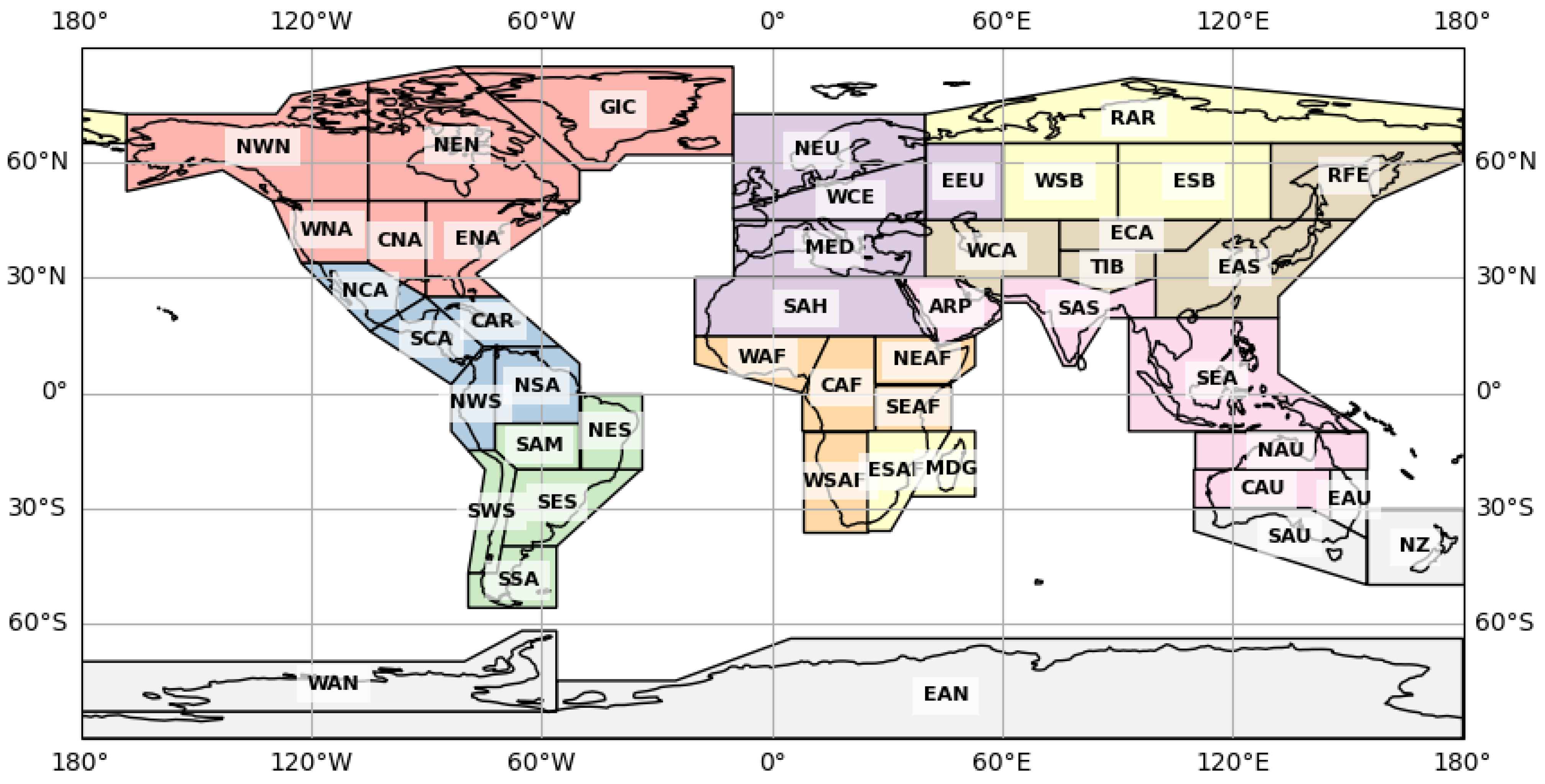
Figure 1. Global land division based on intergovernmental panel on climate change AR6 zoning.
Fractalfract 09 00385 g001
Figure 2. The global distribution of Hurst exponents derived from the WMLE–EMD-DFA method: (a) ATP; (b) AMT; (c) differences between the Hurst exponents of ATP and AMT.
Fractalfract 09 00385 g002
Figure 3. The global distribution of Hurst exponents derived from the R/S analysis method: (a) ATP; (b) AMT; (c) differences between the Hurst exponents of ATP and AMT.
Fractalfract 09 00385 g003
Figure 4. Boxplots of H values for ATP and AMT across global and continental grid points based on different methods: (a) WMLE–EMD-DFA; (b) R/S. Each box represents the interquartile range (IQR), with the median shown as a horizontal line, whiskers extending to 1.5 × IQR, and “×” denotes outliers.
Fractalfract 09 00385 g004
Figure 5. H values based on the WMLE–EMD-DFA method for 45 meteorological stations in (a) China, (b) the U.K., and (c) the U.S., respectively.
Fractalfract 09 00385 g005
Figure 6. H values based on the R/S analysis method for 45 meteorological stations in (a) China, (b) the U.K., and (c) the U.S., respectively.
Fractalfract 09 00385 g006
Figure 7. Comparison of regional middle Hurst values for ATP and AMT with the mean Hurst values of grid-point ATP and AMT series within the same region based on (a) the WMLE–EMD-DFA method and (b) the R/S analysis method.
Fractalfract 09 00385 g007
Figure 8. CDM time series plots of regionally averaged (a) ATP and (b) AMT for the globe and six continents.
Fractalfract 09 00385 g008
Figure 9. CDM series for ATP in the subregions of (a) North America and (b) Africa (the regression coefficients for ATP in each subregion obtained from the multiple linear regressions are presented in parentheses).
Fractalfract 09 00385 g009
Figure 10. CDMs of globally averaged ATP and AMT.
Fractalfract 09 00385 g010
Figure 11. CDMs of regionally averaged ATP and AMT for (a) Africa; (b) Asia; (c) Australia; (d) Europe; (e) North America; (f) South America.
Fractalfract 09 00385 g011
Figure 12. CDMs of regionally averaged ATP and AMT for 12 IPCC-AR6 subregions.
Fractalfract 09 00385 g012
Figure 13. CDMs of ATP and AMT from 12 meteorological stations.
Fractalfract 09 00385 g013
Figure 14. Effects of regionally averaged AMT at large spatial scales on regionally averaged ATP at smaller spatial scales: (a) regional-average ATP in the GIC region and AMT in Africa; (b) regional-average ATP in the CAU region and AMT in Australia.
Fractalfract 09 00385 g014
Figure 15. Log–log plots of the fluctuation function Fq(s) versus scale s for moment orders q ∈ [−5,5], illustrating multifractal cross-correlations between ATP and AMT. All regions exhibit clear power-law behavior, supporting the estimation of generalized cross-Hurst exponents. The position of the lines in each panel varies monotonically with q: curves corresponding to higher q values are consistently positioned higher, while those for lower q values appear lower. The subplots correspond to (a) Globe, (b) Southern Hemisphere, (c) Northern Hemisphere, (d) Africa, (e) Asia, (f) Australia, (g) Europe, (h) South America, and (i) North America.
Fractalfract 09 00385 g015
Figure 16. Generalized cross-Hurst exponent H(q) derived from ATP and AMT.
Fractalfract 09 00385 g016
Table 1. Granger causality test results for ATP and AMT series at 12 IPCC-AR6 subregions and 12 meteorological stations.
RegionLag TimeF Statisticp-ValueStationLag TimeF Statisticp-Value
NEU14.1118 0.0448 Beijing32.10530.1105
CNA10.5652 0.4537 Harbin31.83820.1520
NEN34.8648 0.0032 Wuhan16.29900.0148
NES223.6804 0.0001 Hohhot44.91220.0021
WCE28.6978 0.0003 Aberporth17.88990.0063
NEAF28.3119 0.0004 Eskdalemuir43.17380.0395
WSB31.0103 0.3910 Heathrow15.24130.0254
ECA84.2472 0.0002 Rossonwye42.17380.0795
TIB63.4034 0.0042 Los Angeles20.07030.9322
SEA38.2080 0.0001 Phoenix21.02160.3657
NAU43.7286 0.0070 Dallas82.21940.0323
EEU12.9359 0.0892 San Diego22.66380.0675
Disclaimer/Publisher’s Note: The statements, opinions and data contained in all publications are solely those of the individual author(s) and contributor(s) and not of MDPI and/or the editor(s). MDPI and/or the editor(s) disclaim responsibility for any injury to people or property resulting from any ideas, methods, instructions or products referred to in the content.