Abstract
In this paper, we apply Grünwald–Letnikov-type fractional-order calculus to simulate the growth of Serbia’s gross domestic product (GDP). We also compare the fractional-order model’s results with those of a similar integer-order model. The significance of variables is assessed by the Akaike Information Criterion (AIC). The research demonstrates that the Grünwald–Letnikov fractional-order model provides a more accurate representation compared to the standard integer-order model and performs very accurately in predicting GDP values.
1. Introduction
Differential equations of fractional orders appear in many branches of the sciences. For example, numerous solutions to concrete problems are collected in [1,2,3,4]. Since fractional derivatives are non-local operators, they are commonly used to model memory effects in the system when the independent coordinate represents time. Non-integer-order fractional derivatives have wide applications in various sciences, such as mechanics [5,6], biology [7], economics [8,9], engineering [10], or control theory [11].
Derivatives and integrals are often used to describe the process of economic development. However, classical calculus still has some limitations when it comes to modeling real-world data. On the other hand, fractional calculus is widely used to construct economic models that involve the memory effect in the evolutionary process. Fractional derivatives indeed capture memory effects, meaning that they take into account not only the present state of a system but also its historical behavior. In economics, fractional derivatives allow us to describe processes—for example, when modeling long-term effects of economic changes—where the current state is influenced by a combination of past states rather than only the immediate past (as with traditional integer-order derivatives). In other words, as the fractional derivative of a function is a non-local operator, its value is influenced by the function’s past values. Fractional models have been shown to outperform integer models and serve as superior tools for describing memory in economic growth modeling (EGM), as seen in [12,13,14,15,16]. We mention here that it is well known that EGM is one of the most important models in the study of the dynamics of finance behavior.
Numerous models of GDP growth have been published (for references related to Serbia, see [17,18,19,20]). However, to our knowledge, no fractional model of GDP as a function of an input vector has been developed for Serbia. Motivated by this gap, the objective of this study is to model the growth of Serbia’s national economy through its gross domestic product (GDP) using a fractional-order approach. Specifically, GDP is expressed as a function of nine variables, with the data sources provided in Appendix A.
Thus, in this paper, we apply Grünwald–Letnikov fractional-order and integer-order EGM to study Serbia’s GDP growth, as well as the minimum mean squared error (MSE) criterion to estimate the model parameters. To compare the performance of the integer-order and fractional-order models, we employ mean absolute deviation (MAD), the coefficient of determination (R2 ), and the AIC index.
This paper is structured as follows: Section 2 introduces the Grünwald–Letnikov fractional derivative for reference purposes. Section 3 presents the proposed method for modeling the growth of the Serbian economy. Section 4 presents the results obtained from fitting the model to the Serbian economy and compares them. Finally, Section 5 offers concluding remarks.
2. Fractional Calculus
The facts presented in this section are largely based on [21]. Fractional calculus is the theory of integrals and derivatives of arbitrary order which unify and generalize the notions of integer-order differentiation and n-fold integration. As will be shown, these concepts are more closely related than is typically assumed. In particular, if we consider the infinite sequence of n-fold integrals and n-fold derivatives,
Then, the derivative of arbitrary real order can be considered an interpolation of this sequence of operators, and we will use the notation
Derivatives of arbitrary order are called fractional derivatives. Conversely, the term fractional integrals refers to integrals of arbitrary order and corresponds to negative values of . The fractional integral of order will be denoted by
Subscripts a and t are called terminals, and they denote the two bounds involved in fractional differentiation and integration operations.
The formula
for the first-order derivative of a function can be applied recursively to obtain higher-order derivatives. Specifically, it can be shown that
where
is the usual notation for the binomial coefficients. If we allow n to be a negative integer, then we obtain
which represents the derivative of order n when and the n-fold integral when (for details, see [12,21]). For example, for a negative integer p, that is, , , one obtains (see [21], p. 46)
which is the well-known Cauchy formula for repeated integration. Finally, if we remove the restriction that p must be an integer and redefine the binomial coefficients using the Gamma function as (see [12])
we obtain the so-called direct Grünwald–Letnikov derivative (see [22])
3. Integer and Fractional Model Description
The general expression of the EGM is
where f is a given function, are the variables on which the output depends, and the output model y represents the GDP (in constant 2021 Serbian dinars). The variables on which the output depends are
- : land area (km2);
- : arable land (hectares);
- : population;
- : school attendance (years);
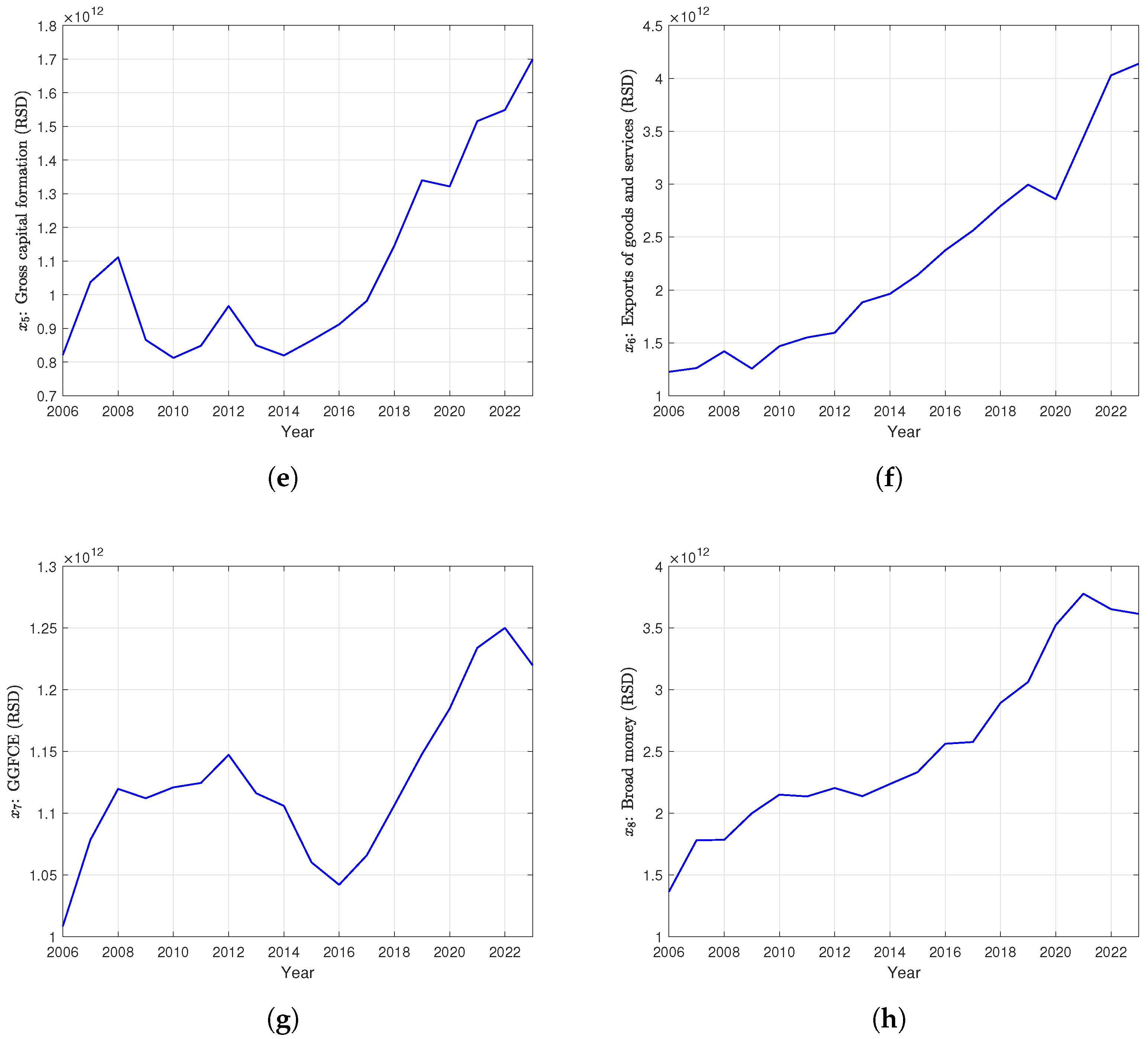
- : gross capital formation (GCF) (constant LCU, 2021 Serbian dinars);
- : exports of goods and services (constant LCU, 2021 Serbian dinars);
- : general government final consumption expenditure (GGFCE) (constant LCU, 2021 Serbian dinars);
- : broad money (constant LCU, 2021 Serbian dinars);
- : variation in gross capital formation (GCF).
A brief explanation of the variable selection is provided below:
- Land area, , is used as a measure of the available natural resources;
- Arable land, , is used as a measure of the quality of natural resources;
- Population, , is used as a measure of the available human resources;
- School attendance, , is used as a measure of the quality of human resources;
- Manufactured resources are represented by ;
- Exports, , are used as a measure of external impacts on the economy;
- GGFCE, , is used as a measure of budgetary impacts on the economy;
- is used as a measure of monetary impacts on the economy;
- is used as a measure of the impact of investment on the economy.
We note that GCF appears twice in the model, each time representing a different economic aspect, and it is thus assigned two distinct variables, and , to ensure precision. These variables are also used in [12].
While the selection of the nine variables in our model is guided by both Keynesian short-term inputs and long-term growth accounting principles [23,24], in the following, we provide the rationale for their selection, specifically in relation to their relevance in the Serbian economy:
- (land area) and (arable land) are not only general measures of resources but are also important due to their relatively high share in gross value added and total employment of agriculture in the Serbian economy [25], especially in certain regions. Agriculture plays a critical role contributing to both domestic consumption and export capacity [26].
- (population) and (school attendance in years) represent the quantity and quality of the labor force. Indeed, workforce migration is an important constraint [27,28], influencing labor supply and domestic consumption. Investment in education and research and development [29] has often been recognized as essential for long-term GDP and productivity growth, although education as an indicator has limitations in the short term, as emphasized later on in this paper when discussing the results.
- (GCF) and (variation of GCF) record both the accumulation and dynamics of investments, crucial in the transition phase and after crises (e.g., 2008, 2020). Foreign direct investment still plays a crucial role in Serbia’s economic development, particularly in sectors like manufacturing and technology, as it facilitates not only technology transfer but general capital inflows that contribute to infrastructure development and unemployment rate decrease [20].
- (exports of goods and services) and (GGFCE) were chosen as representatives of external and fiscal impulses, which are significant in a small open economy like Serbia. Despite challenges in the EU accession process, Serbia’s efforts to integrate into regional and global markets put both the import and export of goods and services as a fundamental factor for GDP growth. In particular, in recent years, Serbia became recognized by its export of information and communication technology services [30].
- (broad money) was taken as a monetary indicator, taking into account the role of exchange rate stability and inflation in the transition period.
Thus, the integer-order model (IOM) and its generalization to a non-integer-order, namely the Grünwald–Letnikov fractional-order model (GLFOM), are considered as
- IOM:
- GLFOM:
4. Optimization and Performance Evaluation
In this section, we present an application of the model introduced in the previous section by analyzing the economic growth of Serbia over the period of 2006 to 2023. This period was selected because Serbia became an independent country, following its separation from Montenegro, in 2006.
4.1. Economic Data for Serbia
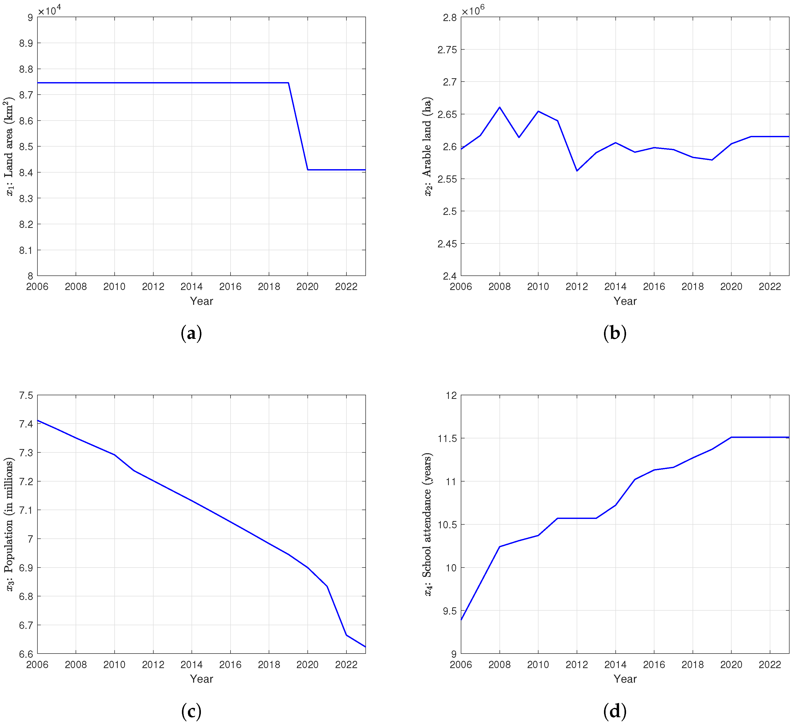
Using Serbian economic data from 2006 to 2023 in constant local currency units, we used MATLAB 2021a to generate Figure 1 (see also Table A1 in Appendix A).
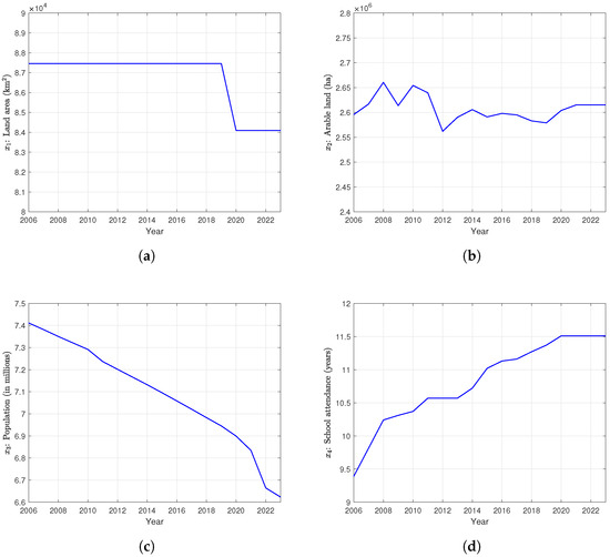
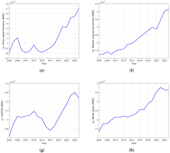
Figure 1.
Data for Serbia from 2006 to 2023, where RSD is the currency of Serbia (Serbian dinar).
4.2. Parameter Estimation
The goal of the estimation process is to compute the numerical parameters—namely the coefficients and the orders , —of the proposed models (1) and (2) for the Serbian economy. Notice that, in the case of the IOM, the orders are fixed: the order of is , the orders of and are 1, and the orders of all other variables are 0, as explained in Section 2.
The parameter estimation procedure is carried out in MATLAB. The coefficients are computed using the least squares method, as this constitutes a standard linear data fitting problem, whereas the orders are estimated using the Nelder–Mead simplex search method, implemented via the fminsearch function. This method minimizes the mean squared error (MSE), defined as
where n is the number of years (in our case, ), and and denote the actual GDP (real output) and the model-estimated GDP (model output), respectively. The resulting values are shown in Table 1.

Table 1.
The coefficients and the orders of the integer-order model (IOM) and the Grünwald–Letnikov fractional-order model (GLFOM).
4.3. Model Evaluation
Since the MSE alone is not sufficient to evaluate the quality of the models, additional performance metrics are calculated to assess the goodness of fit and to compare the performance of the IOM and GLFOM models. These are
- The mean absolute deviation (MAD), given by
- The coefficient of determination (), given by
As will be shown below, not all derivative orders in the GLFOM model need to be adjusted relative to the IOM. This will be evaluated by examining whether performance indices such as the MSE, MAD, and significantly deteriorate when a given derivative order is left unchanged, i.e., retained from the IOM. For this purpose, the Akaike Information Criterion (AIC) is also used, defined as
where m is the number of parameters in the model.
Table 2.
Performance indices for the Serbian economy.
It is important to note that the Akaike Information Criterion (AIC) is used primarily for model selection rather than for directly assessing model quality. The absolute value of the AIC alone does not provide information about the goodness of fit. However, by comparing the AIC values of different models, we can identify which models are more likely to fit the data well. Specifically, a lower AIC value indicates a higher likelihood that the model is the best among the candidates. Additionally, given L competing models, the Akaike weights, defined by
provides the probability that model i is the best among the L competing models. The importance of each variable was then assessed and represented by the corresponding Akaike weight w (see Table 3).
Table 3.
Variable importance based on AIC.
One can see that there is absolutely no improvement in the models by removing any variables. More precisely, the value of 0% indicates that the probability of the model without the k-th variable being the best is nil; consequently, these models without one variable should not be chosen, or in other words, no variables should be excluded from the original model. The reason why all Akaike weights in Table 3 are equal to zero when any variable is omitted is that compared to the full model, all reduced models perform significantly worse in terms of their AIC values. These uniformly zero weights reflect that each variable makes a significant contribution to explaining GDP, and omitting any one of them leads to a considerable decline in fit quality. Nonetheless, we acknowledge that with small datasets, criteria like the AIC can exhibit sharp changes in relative weights. Therefore, we interpret these results with caution: while all variables are retained, their actual influence is better understood when considered alongside the derivative orders, as discussed later in Table 4.
Table 4.
Derivative orders importance based on AIC.
Next, we examined the influence of the derivative orders on the results and found (see also Table 1) that when the variables and have order 0 (i.e., without derivatives), the Akaike weights indicate probabilities of 23.26% and 24.17%, respectively, for these models to be the best compared to all others, including those with one variable excluded (see Table 4). Additionally, the Akaike weight for the GLFOM model is 24.06%. Although a slight deterioration in the MAD is observed, the results obtained with the fractional model where remain highly satisfactory. Specifically, the AIC values show that this model has the highest probability of being the best among all considered models. Furthermore, despite a small deterioration in the MSE and MAD for the model with , this model also demonstrates excellent performance.
Given that only economic indicators with affect GDP over time, despite the expectation that years of school attendance should have a long-term impact on GDP (see, for example, [31]), it was found that school attendance () and exports of goods and services () have little influence on GDP, similarly to findings for several countries reported in [32]. This may simply be due to the relatively short period under consideration (see [33]). Furthermore, the impact of education on GDP often unfolds with a significant time lag. Individuals currently in school will not enter the labor force for several years, and even after entering, the economic benefits of their education—such as enhanced skills and productivity—may take additional time to materialize and influence overall economic output. As for exports, it can be noted that Serbian exports often have low domestic added value, meaning that raw materials or semi-processed products do not significantly impact GDP. Additionally, a considerable share of export revenues is captured by foreign-owned companies operating within the country, resulting in profits not being retained within the local economy. This limits the overall contribution of exports to GDP, as the positive effects on domestic consumption, investment, and employment remain constrained.
It is very important to note one key aspect regarding our use of Akaike weights. Specifically, we simultaneously calculated the Akaike weights for all the mentioned models, including the models excluding one variable (see Table 3), the models without changes in derivative orders (see Table 4), the IOM with all variables (0%), and the GLFOM with all variables (24.06%).
We also calculated the MSE, MAD, and R2 for models where for (see Table 5; for a better overview, we re-state the corresponding data from Table 2).
Table 5.
Performance indices for the Serbian economy for different models.
4.4. Fitting Results
We now present the fitting results for the IOM and the GLFOM, as well as for two modified versions of the GLFOM where the derivative orders for and are set to zero (i.e., and ) separately. These results were generated using MATLAB software (see Figure 2).
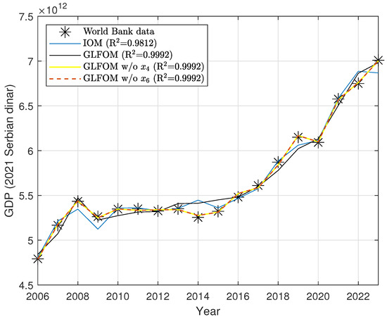
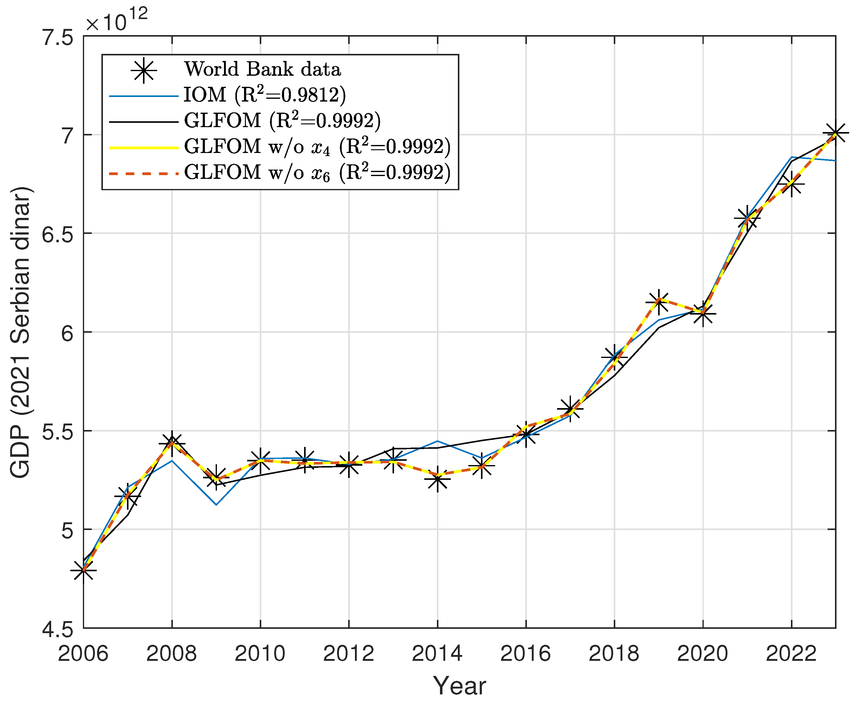
Figure 2.
Fitting results for the IOM and the GLFOM, where w/o and w/o mean that and have a zero-order derivative.
Figure 2 illustrates how closely each model’s predicted GDP values align with the actual GDP data for Serbia from 2006 to 2023. The figure provides a visual comparison between the real GDP values (denoted by *) and the predictions of four models, namely the integer-order model (IOM), the full Grünwald–Letnikov fractional-order model (GLFOM), and two simplified variants of the GLFOM in which the fractional orders for variables (school attendance) and (exports of goods and services) are set to zero, respectively. The figure shows that the GLFOM provides a significantly closer fit to the actual GDP values than the IOM. This confirms the superior descriptive capability of fractional derivatives in modeling economic growth, as also supported by the statistical indices reported earlier. The GLFOM curve follows the actual values more closely, even in the face of significant economic disturbances like the COVID-19 pandemic.
4.5. Prediction Results
Finally, we present the forecasted results for Serbia’s GDP data from 2016 to 2023 using the IOM and GLFOM models. We calculated one-year-ahead predictions from models built with 10 years of data. Specifically, we used the period from 2006 to 2015 as the initial training sample to predict GDP for the year 2016. Subsequently, we expanded the training sample by one year at a time using the period of 2007 to 2016 to predict GDP for the year 2017; using the period of 2008 to 2017 to predict GDP for the year 2018; and so on, until finally using the period of 2013 to 2022 to predict GDP for the year 2023.
In addition, we computed the corresponding absolute relative error (ARE) index values to assess and compare the models’ prediction accuracy and effectiveness, as shown in Table 6.
Table 6.
Real and predicted GDP values for Serbia.
We note that the absolute relative error (ARE) criterion is defined as
Table 6 shows that for all years except the last two, the prediction results obtained using the GLFOM are significantly more accurate than those obtained by the IOM. In particular, the most accurate prediction occurred in 2020, which coincides with the onset of the COVID-19 pandemic and the associated lockdowns. This is especially notable given the high level of uncertainty during that period. Overall, even from the perspective of prediction accuracy, the fractional-order model proves to be superior to the classical integer-order model.
5. Conclusions
This paper develops economic growth models for Serbia over the period of 2006 to 2023. We employed both the IOM and GLFOM models to analyze Serbia’s GDP growth, using nine economic indicators as input variables. The fitting results demonstrated that the GLFOM model significantly outperformed the IOM model. A comprehensive comparison of the two models was conducted using various statistical tools. To further emphasize the forecasting capabilities of the GLFOM model, we presented one-year-ahead GDP forecasts for Serbia from 2016 to 2023 and compared them with the actual values. The results indicate that the GLFOM model not only provides a better fit to Serbia’s GDP data but also delivers more accurate predictions.
Not only methodological innovations in assessing economic growth but also policy recommendations can be offered by this research, since by recognizing the most important influences on economic growth, a few recommendations can be outlined. Although school attendance was not found to be a significant determinant of GDP in this study, its long-term potential through improvements in human capital should not be overlooked. Therefore, policymakers might consider enhancing the quality of education and its alignment with labor market needs to support future productivity gains. However, the economic impact of such measures would likely manifest only over the long term. Similarly, while exports did not emerge as a key factor in this analysis, further research into their structure, ownership, and local reinvestment could provide insights into their broader economic relevance.
Author Contributions
Conceptualization, E.K., D.V., and L.R.; methodology, D.V. and E.K.; software, D.V. and E.K.; resources, L.R. and D.V.; writing—original draft preparation, E.K.; writing—review and editing, E.K., D.V., and L.R.; project administration, D.V.; funding acquisition, D.V. All authors have read and agreed to the published version of the manuscript.
Funding
The authors acknowledge Fundação para a Ciência e a Tecnologia (FCT) for its financial support via the project LAETA Base Funding (DOI: 10.54499/UIDB/50022/2020).
Data Availability Statement
The original contributions presented in this study are included in the article. Further inquiries can be directed to the corresponding author.
Conflicts of Interest
The authors declare no conflicts of interest. The funders had no role in the design of the study; in the collection, analyses, or interpretation of data; in the writing of the manuscript; or in the decision to publish the results.
Abbreviations
The following abbreviations are used in this manuscript:
| GDP | Gross domestic product |
| AIC | Akaike Information Criterion |
| EGM | Economic growth modeling |
| MSE | Mean squared error |
| MAD | Mean absolute deviation |
| GCF | Gross capital formation |
| GGFCE | General government final consumption expenditure |
| LCU | Local currency unit |
| IOM | Integer-order model |
| GLFOM | Grünwald–Letnikov fractional-order model |
| RSD | Republic of Serbia dinar |
| ARE | Absolute relative error |
Appendix A
The economic data presented in this paper are provided in Table A1. The sources of the data in this table are as follows:
- The values for variables , , , , , , and are taken from [34]. The values of land area () for 2023 were assumed to be the same as for the period of 2006–2022. Similarly, the values of arable land () for 2022 and 2023 were assumed to be equal to its 2021 values;
- The values for variable are taken from [35], with the values for 2023 assumed to be the same as in 2022.
Table A1.
Serbian economic data for the period of 2006–2023.
References
- Oldham, K.B.; Spanier, J. The Fractional Calculus; Academic Press: New York, NY, USA, 1974. [Google Scholar]
- Miller, K.S.; Ross, B. An Introduction to the Fractional Calculus and Fractional Differential Equations; John Wiley & Sons: New York, NY, USA, 1993. [Google Scholar]
- Samko, S.G.; Kilbas, A.A.; Marichev, O.I. Fractional Integrals and Derivatives; Gordon and Breach: Amsterdam, The Netherlands, 1993. [Google Scholar]
- Kilbas, A.A.; Srivastava, H.M.; Trujillo, J.I. Theory and Applications of Fractional Differential Equations; Elsevier: Amsterdam, The Netherlands, 2006. [Google Scholar]
- Atanackovic, T.M.; Kacapor, E.; Djekic, D.D.; Gilic, E. Non-local wave equation: Time delay with second order terms. Z. Angew. Math. Mech. 2025, 105, e202401241. [Google Scholar] [CrossRef]
- Atanackovic, T.M.; Djekic, D.D.; Gilic, E.; Kacapor, E. On a Generalized Wave Equation with Fractional Dissipation in Non-Local Elasticity. Mathematics 2023, 11, 3850. [Google Scholar] [CrossRef]
- Nonnenmacher, T.F.; Metzler, R. Applications of Fractional Calculus Ideas to Biology, in Applications of Fractional Calculus in Physics; World Scientific: Singapore, 1998. [Google Scholar]
- Scalas, E.; Gorenflo, R.; Mainardi, F. Fractional calculus and continuous-time finance. Phys. A Stat. Mech. Its Appl. 2000, 284, 376–384. [Google Scholar] [CrossRef]
- Laskin, N. Fractional market dynamics. Phys. A Stat. Mech. Its Appl. 2000, 287, 482–492. [Google Scholar] [CrossRef]
- Tenreiro Machado, J.A.; Silva, M.F.; Barbosa, R.S.; Jesus, I.S.; Reis, C.M.; Marcos, M.G.; Galhano, A.F. Some Applications of Fractional Calculus in Engineering. Math. Probl. Eng. 2010, 2010, 639801. [Google Scholar] [CrossRef]
- Podlubny, I. Fractional-Order Systems and Fractional-Order Controllers; Tech. Report UEF-03-94; Institute for Experimental Physics, Slovak Academy of Sciences: Kosice, Slovakia, 1994. [Google Scholar]
- Tejado, I.; Valério, D.; Pérez, E.; Valério, N. Fractional calculus in economic growth modelling: The Spanish and Portuguese cases. Int. J. Dyn. Control 2017, 5, 208–222. [Google Scholar] [CrossRef]
- Machado, J.A.T.; Mata, M.E. A fractional perspective to the bond graph modelling of world economies. Nonlinear Dyn. 2015, 80, 1839–1852. [Google Scholar] [CrossRef]
- Škovránek, T.; Podlubny, I.; Petráš, I. Modeling of the national economies in state-space: A fractional calculus approach. Econ. Model. 2012, 29, 1322–1327. [Google Scholar] [CrossRef]
- Ming, H.; Wang, J.; Fečkan, M. The Application of Fractional Calculus in Chinese Economic Growth Models. Mathematics 2019, 7, 665. [Google Scholar] [CrossRef]
- Tejado, I.; Hernández, E.; Valério, D. Economic growth in the European Union modelled with fractional derivatives: First results. Bull. Pol. Acad. Sci. Tech. Sci. 2018, 66, 455–465. [Google Scholar]
- Mitić, P.; Kojić, M.; Minović, J.; Stevanović, S.; Radulescu, M. An EKC-based modelling of CO2 emissions, economic growth, electricity consumption and trade openness in Serbia. Environ. Sci. Pollut. Res. 2024, 31, 5807–5825. [Google Scholar] [CrossRef] [PubMed]
- Obradovic, S.; Sapic, S.; Furtula, S.; Lojanica, N. Linkages between Inflation and Economic Growth in Serbia: An ARDL Bounds Testing Approach. Eng. Econ. 2017, 28, 401–410. [Google Scholar] [CrossRef]
- Uvalić, M.; Cerović, B.; Atanasijević, J. The Serbian economy ten years after the global economic crisis. Econ. Ann. 2020, 65, 33–71. [Google Scholar] [CrossRef]
- Vukmirović, V.; Kostić Stanković, M.; Pavlović, D.; Ateljević, J.; Bjelica, D.; Radonić, M.; Sekulić, D. Foreign Direct Investments’ Impact on Economic Growth in Serbia. J. Balk. Near East. Stud. 2021, 23, 122–143. [Google Scholar] [CrossRef]
- Podlubny, I. Fractional Differential Equations: An Introduction to Fractional Derivatives, Fractional Differential Equations, to Methods of Their Solution and Some of Their Applications, 1st ed.; Academic Press: San Diego, CA, USA, 1998. [Google Scholar]
- Ortigueira, M.D.; Coito, F. From differences to derivatives. Fract. Calc. Appl. Anal. 2004, 7, 459–471. [Google Scholar]
- Denison, E.F. Why Growth Rates Differ: Post-War Experience in Nine Western Countries; Brooking Institutions: Washington, DC, UDA, 1967. [Google Scholar]
- Lucas, R.E. On the mechanics of economic development. J. Monet. Econ. 1988, 22, 3–42. [Google Scholar] [CrossRef]
- Mijatović, B.; Zavadjil, M. Serbia on the path to modern economic growth. Econ. Hist. Rev. 2023, 76, 199–220. [Google Scholar] [CrossRef]
- Stojanović, Ž. Agriculture in Serbia. In The Geography of Serbia: Nature, People, Economy; Manić, E., Nikitović, V., Djurović, P., Eds.; Springer International Publishing: Cham, Switzerland, 2022; pp. 199–206. [Google Scholar] [CrossRef]
- Drobnjaković, M.; Panić, M.; Kanazir, V.K.; Javor, V. Spatial aspects of labor force formation: The interrelation of cohort turnover and net migration in Serbia. Eurasian Geogr. Econ. 2022, 63, 543–559. [Google Scholar] [CrossRef]
- Lukić, V. Migration and mobility patterns in Serbia. In The Geography of Serbia: Nature, People, Economy; Manić, E., Nikitović, V., Djurović, P., Eds.; Springer International Publishing: Cham, Switzerland, 2022; pp. 157–167. [Google Scholar] [CrossRef]
- Kutlača, D.; Šestić, S.; Jelić, S.; Popović-Pantić, S. The impact of investment in research and development on the economic growth in Serbia. Industrija 2020, 48, 23–46. Available online: https://aseestant.ceon.rs/index.php/industrija/article/view/24949 (accessed on 12 June 2025).
- Domazet, I.; Marjanović, D.; Ahmetagić, D. The impact of high-tech products exports on economic growth—The case of Serbia, Bulgaria, Romania and Hungary. Ekon. Preduz. 2022, 70, 191–205. [Google Scholar] [CrossRef]
- Agasisti, T.; Bertoletti, A. Higher education and economic growth: A longitudinal study of European regions 2000–2017. Socio-Econ. Plan. Sci. 2022, 81, 100940. [Google Scholar] [CrossRef]
- Tejado, I.; Pérez, E.; Valério, D. Fractional Derivatives for Economic Growth Modelling of the Group of Twenty: Application to Prediction. Mathematics 2020, 8, 50. [Google Scholar] [CrossRef]
- Breton, T.R.; Siegel Breton, A. Education and Growth: Where All the Education Went; Working Papers, No. 16-02; Center for Research in Economics and Finance (CIEF): George Mason, VA, USA, 2016. [Google Scholar] [CrossRef]
- World Bank Group. File: API_SRB_DS2_en_excel_v2_17914.xls. Available online: https://data.worldbank.org/country/serbia?view=chart (accessed on 18 April 2025).
- Global Data Lab. File: GDL-Mean-Years-Schooling-Data.xlsx. Available online: https://globaldatalab.org/shdi/table/msch/SRB/?levels=1+4&interpolation=0&extrapolation=0 (accessed on 18 April 2025).
Disclaimer/Publisher’s Note: The statements, opinions and data contained in all publications are solely those of the individual author(s) and contributor(s) and not of MDPI and/or the editor(s). MDPI and/or the editor(s) disclaim responsibility for any injury to people or property resulting from any ideas, methods, instructions or products referred to in the content. |
© 2025 by the authors. Licensee MDPI, Basel, Switzerland. This article is an open access article distributed under the terms and conditions of the Creative Commons Attribution (CC BY) license (https://creativecommons.org/licenses/by/4.0/).