1. Introduction
Stability is a fundamental concept with broad applications across multiple disciplines, playing a vital role in ensuring the resilience and reliability of systems. In civil engineering, it ensures that structures can withstand environmental stresses, thereby guaranteeing safety and durability. Similarly, aerospace engineering depends on stability to maintain aircraft control during flight, which is critical for passenger safety. In control systems and robotics, stability principles guide the design of algorithms that enable machines to respond effectively to disturbances [
1].
In finance, stability concepts help investors manage risk and achieve consistent returns in fluctuating markets. Environmental scientists apply stability theories to understand and predict ecosystem behavior, which offers valuable insights for conservation efforts. In software development, stability ensures that applications perform reliably under varying conditions. Likewise, electrical engineering uses stability analyses to maintain balance in power systems and minimize outages [
2].
In psychology, the stability of therapeutic frameworks supports the development of techniques that foster emotional resilience. In network design, maintaining stability ensures consistent data flows in telecommunications systems. Mechanical engineers also rely on stability principles to design safe, efficient machines capable of operating in dynamic environments. Overall, stability is critical for optimizing performance, enhancing safety, and ensuring sustainability across a wide range of fields [
3].
In mathematics, stability primarily addresses the qualitative behavior of solutions to mathematical problems, particularly differential equations. It concerns how small changes in initial conditions or parameters influence the behavior of solutions over time. A foundational concept in this area is Lyapunov stability, which helps determine whether a system returns to its equilibrium state after experiencing a disturbance [
4].
In this context, an equilibrium point is considered stable if solutions that start near it remain close at all future times. This principle is pivotal in control theory, where engineers examine a system’s responses to inputs and perturbations to ensure its desired performance.
In numerical analysis, stability is essential for ensuring the accuracy of computational methods. Stable algorithms yield consistent and reliable results, even when inputs are slightly altered, making them indispensable in simulations and real-world modeling [
5].
The insights gained from stability analyses extend across disciplines—from physics to economics—allowing researchers to predict and understand complex behaviors in dynamic systems. Mathematical tools such as stabilizing feedback mechanisms, regularization techniques, and robustness methods help reinforce stability across applications. Ultimately, the study of stability in mathematics underpins both theoretical and practical advancements in the analysis and control of dynamic systems [
6,
7].
To provide a recent overview of fractional differential and difference equations, we will survey the following selected studies:
D. Otrocol and V. Ilea’s work [
8], which explored the concepts of UH stability and generalized UH–Rassias stability for a specific delay differential equation,
J. Wang and Y. Zhang’s [
9] study, which established some findings regarding the existence, uniqueness, and UHML stability of Caputo-type fractional differential equations:
Liu et al.’s work, found in [
10], which demonstrated the existence, uniqueness, and UHML stability of solutions for a certain class of
-Hilfer fractional differential equations:
K.D. Kucche and P.U. Shikhare’s study [
11], which examined the existence and uniqueness of solutions, as well as Ulam-type stabilities, for Volterra delay integro-differential equations defined on a finite interval:
And Ref. [
12], where the authors established the existence, uniqueness, and UHML stability of solutions for a class of
-Hilfer problems related to fractional differential equations with infinite delay:
For more detailed information on existing research related to the stability of fractional systems and the existence and uniqueness of solutions, please refer to references [
13,
14,
15]. These works offer comprehensive insights into the theoretical foundations and recent developments in this field. They also examine various analytical methods and stability criteria essential for understanding the behavior of fractional differential equations. Reviewing these sources will provide a solid background and context for the current study.
In references [
16,
17], the authors introduce several special functions and explore their interrelations. They use these functions to propose a new concept of stability known as multi-stability. This type of stability proves particularly useful in optimizing stability-related problems, especially within the framework of fractional calculus.
Building on the insights from these foundational sources [
12,
16,
17], we present a study on the stability of fractional systems with infinite delay, emphasizing their effectiveness in modeling complex dynamic behavior and exploring recent advances in the existence and types of stability of solutions. Utilizing methods such as the Picard operator approach, Banach’s fixed-point theorem, a generalized Gronwall inequality, and various special functions, we derive key stability conditions for systems involving Hadamard fractional derivatives. Numerical examples and graphical illustrations demonstrate that fractional-order control significantly enhances system stability and robustness compared to conventional integer-order methods.
In this paper, the deep connection between fractional calculus and special functions is clearly evident. We emphasize the important role that special functions play in optimizing our problem. These functions often serve as fundamental tools for expressing solutions to complex problems, enabling precise the modeling of intricate behaviors and enhancing the efficiency of optimization processes. Their well-established properties facilitate analytical solutions, often simplifying numerical computations and ultimately leading to more accurate and reliable results across a wide range of optimization scenarios.
2. Preliminaries
In this section, we present the definitions and auxiliary lemmas that will be used in the main results. In line with the Hadamard fractional derivatives employed in this work, we begin by introducing an associated weighted function space tailored to this framework. We then establish several essential properties of fractional derivatives and integrals involving the natural logarithm function. Finally, we introduce the key analytical tools necessary for studying the existence, uniqueness, and stability of their solutions.
2.1. Special Functions
For every
and
the Wright function
the one-parameter Mittag–Leffler function
and the hypergeometric function
are defined as follows [
16]:
and
2.2. Weighted Spaces
We let
, and
Consider the space of absolutely continuous functions
given on
Now, we define them for
Suppose
and
illustrate the weighted spaces defined as
and
with the following norms
and
respectively.
2.3. Hadamard Derivatives
Let
and
The Hadamard derivative of order
is given as follows [
16]:
where
Below are several properties of fractional derivatives and integrals, including those of the Hadamard fractional derivative.
Lemma 1 ([
9,
12]).
Let , We obtain the following:- (R1)
Let and Then, - (R2)
Let and Then, - (R3)
Let and Then,
- (R4)
Let Then, is bounded on
- (R5)
Let be a continuous function. Then, for the fractional-order problem - (R6)
Let be integrable functions and C be continuous on If, for all Furthermore, if B is a nondecreasing function on then where is the one-parameter Mittag–Leffler function.
2.4. Picard Operators
Consider the metric space Now, is called a Picard operator if there is a s.t., in which and also for , for every
Below is an application of the Picard operator.
Lemma 2 ([
9,
18]).
Assume is an ordered metric space and is an increasing Picard operator with Then, implies and implies ; here, 2.5. Admissible Phase Spaces
A linear topological space of a function from
to
with seminorm
is called an admissible phase space if
B has the following properties [
19,
20]:
- (1)
If is continuous on and then for every we know that:
(1-1) where (here, represents the history of the state from time up to time
(1-2) There exists a with and for .
(1-3) where is continuous, and is locally bounded. We set ,
- (2)
For the function defined in (1), the function is continuous from to
- (3)
B is complete.
In the following, we will study the uniqueness and stability of a new fractional-order system involving the Hadamard fractional derivatives using Banach’s contractive principle and Picard operators and we will give an illustrative example and examine other control functions.
3. Main Results
It is well known that fractional calculus is an emerging tool which uses fractional differential and integral equations to develop more sophisticated mathematical models that can accurately describe complex systems. There are many definitions of fractional derivatives available in the literature, such as the Riemann–Liouville derivative, which plays an important role in the development of the theory of fractional analysis. Another commonly used one is the Hadamard fractional derivative; for studies related to the existence, uniqueness, and stability of solutions for fractional boundary value problems in Hadamard differential equations see [
21,
22].
The Hadamard fractional derivative is distinguished by its intrinsic scale-invariant nature, which is primarily due to its logarithmic kernel. This feature allows it to effectively model processes that exhibit multiplicative or fractal behavior. Unlike the Riemann–Liouville derivative, which often complicates the specification of initial conditions due to its non-zero derivative of constants, the Hadamard derivative more naturally accommodates initial values when appropriately formulated. While the Caputo derivative also facilitates physically interpretable initial conditions, the Hadamard derivative offers a distinct advantage in modeling systems where the underlying dynamics are governed by scale transformations rather than additive processes.
In comparison to the Kilbas–Hilfer derivative—a flexible formulation that interpolates between the Riemann–Liouville and Caputo derivatives—the Hadamard derivative provides a more direct framework for problems emphasizing multiplicative scale invariance rather than varying degrees of memory effects. Although Hilfer’s approach introduces adaptability through a tunable parameter, the Hadamard derivative captures the essence of multiplicative self-similarity via its explicit logarithmic kernel, avoiding the need for additional parameters and offering a more straightforward modeling approach for scale-dependent phenomena. For example, the Hadamard derivative is particularly useful in modeling phenomena such as financial markets or biological growth processes that exhibit scale invariance, as it simplifies the analysis by directly incorporating the natural logarithmic relationships inherent in these systems [
16].
Moreover, compared to the Riemann–Liouville derivative, the Hadamard framework aligns more naturally with systems characterized by power-law and fractal behaviors. It offers meaningful interpretations of phenomena across diverse scientific fields such as physics, finance, and biology, where the evolution of a system depends on multiplicative—rather than additive—factors. By incorporating these features while retaining the analytical strengths of fractional calculus, such as memory effects and nonlocal interactions, the Hadamard derivative becomes a powerful tool for modeling complex multiscale systems.
In essence, the Hadamard fractional derivative’s principal advantage lies in its ability to combine the benefits of fractional calculus with a structure that inherently respects scale invariance—something that is often challenging to achieve with the Riemann–Liouville or Caputo derivatives. While those are generally suited to systems with additive or linear memory dynamics, the Hadamard derivative excels in contexts where multiplicative behavior predominates, offering a more natural, accurate, and intuitive mathematical framework for such problems [
23].
We consider the Banach space
with the norm
In this section, we investigate the stability of the following fractional-order system:
where
and
Theorem 1. Assume the following:
- (A1)
Let be a continuous function; there is a positive constant s.t., for every and such that we have
- (A2)
Let in which and is defined in Section 2.5. - (A3)
Let
-
Then, the fractional-order system has the following properties (1):
- (T1)
A unique solution in
- (T2)
Stability.
Proof. (T1). Notice that
, given by
is a solution of (
1) if
, with the conditions
for every
and
Let
be given by
Let
and consider
which is given by
and so,
For
when
consider
given by
Suppose
satisfies the following integral equation:
and
for
. It is easy to see that
for
iff
satisfies
and
with
We now consider
For
let
Note that
is a Banach space and we can let
be given by
and
for
We now show that
has a unique fixed point. Let
For
we find that
Thus,
when
Assume
and
. Then,
Therefore,
so
is a contraction. The Banach fixed-point theorem guarantees that
has a unique fixed point
Let
and note that
has a unique fixed point
Hence, we obtain the desired result.
(T2) Let
be the solution of (
1) in
with
and let
satisfy the inequality
,
where
Note that the function
is a solution of
if there is a function
s.t.,
for
and
for
Recall the fractional-order system (
1) is stable [
16] with respect to
if there is a
s.t., for every
and every solution
to the inequality
there is a solution
to (
1) with
Observe that if
satisfies the inequality (
6), then
is a solution of the integral inequality
Now, we consider
, the unique solution to the fractional-order system
In a similar way to that in (T1), we obtain
For every
consider
given by
We now show that
is a Picard operator. For every
and
,
we know that
Thus,
is a contraction mapping on
From the Banach fixed-point theorem applied to
we observe that
is a Picard operator and
For every
This implies that
is strictly increasing and, from (A3), we obtain
Applying Lemma 1, for
we obtain
in which
Setting
we obtain
Making use of Lemma 2, we conclude that
Then, for every
Hence, we obtain the desired result. □
Example 1. Employing the values provided in [12,16], we considerwith the norm Consider the fractional-order system (
1)
, which is as follows: for ; for ; ; ; and For every and every we obtain Also,
For every consider the inequality Applying the previous results, we obtain
We will examine other special control functions, specifically the exponential function , the Mittag–Leffler function and the hypergeometric function in place of for different values of
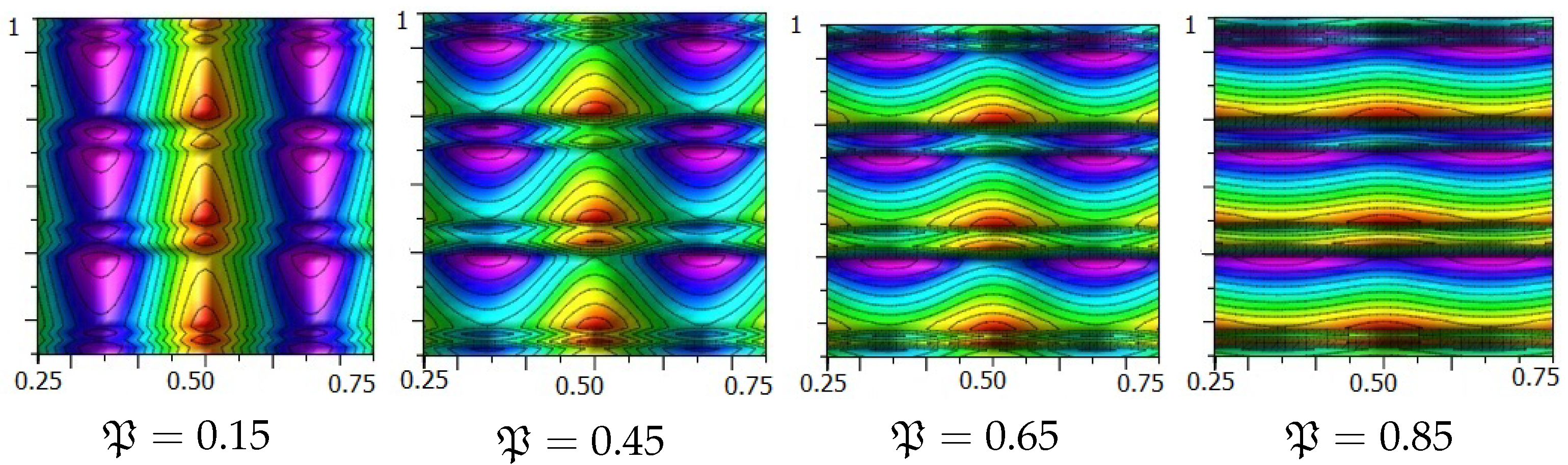
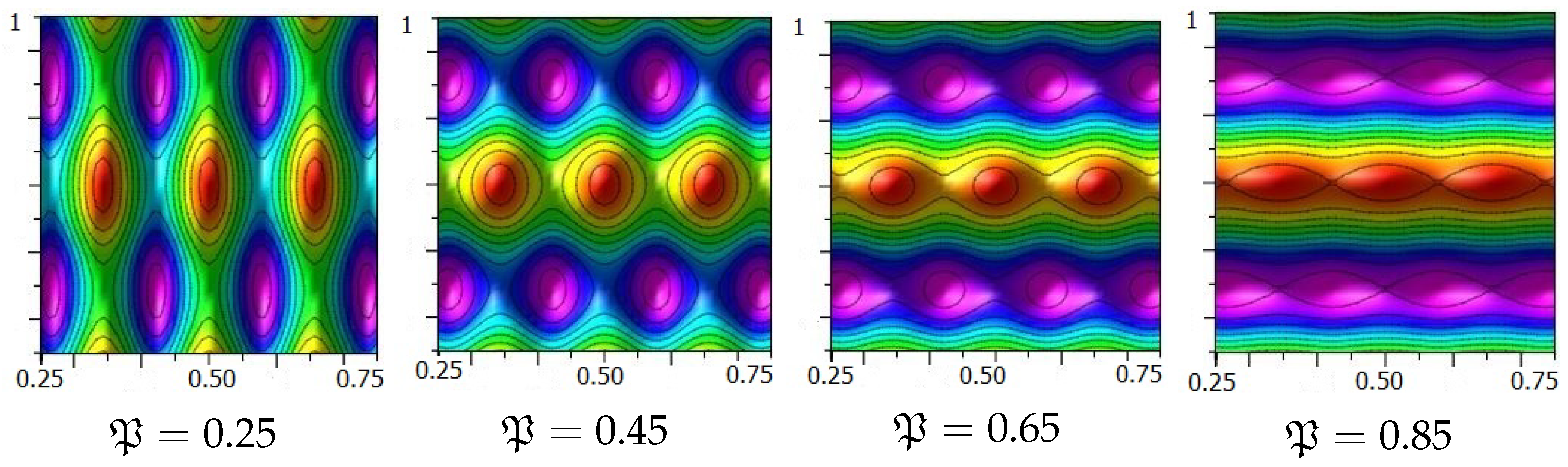
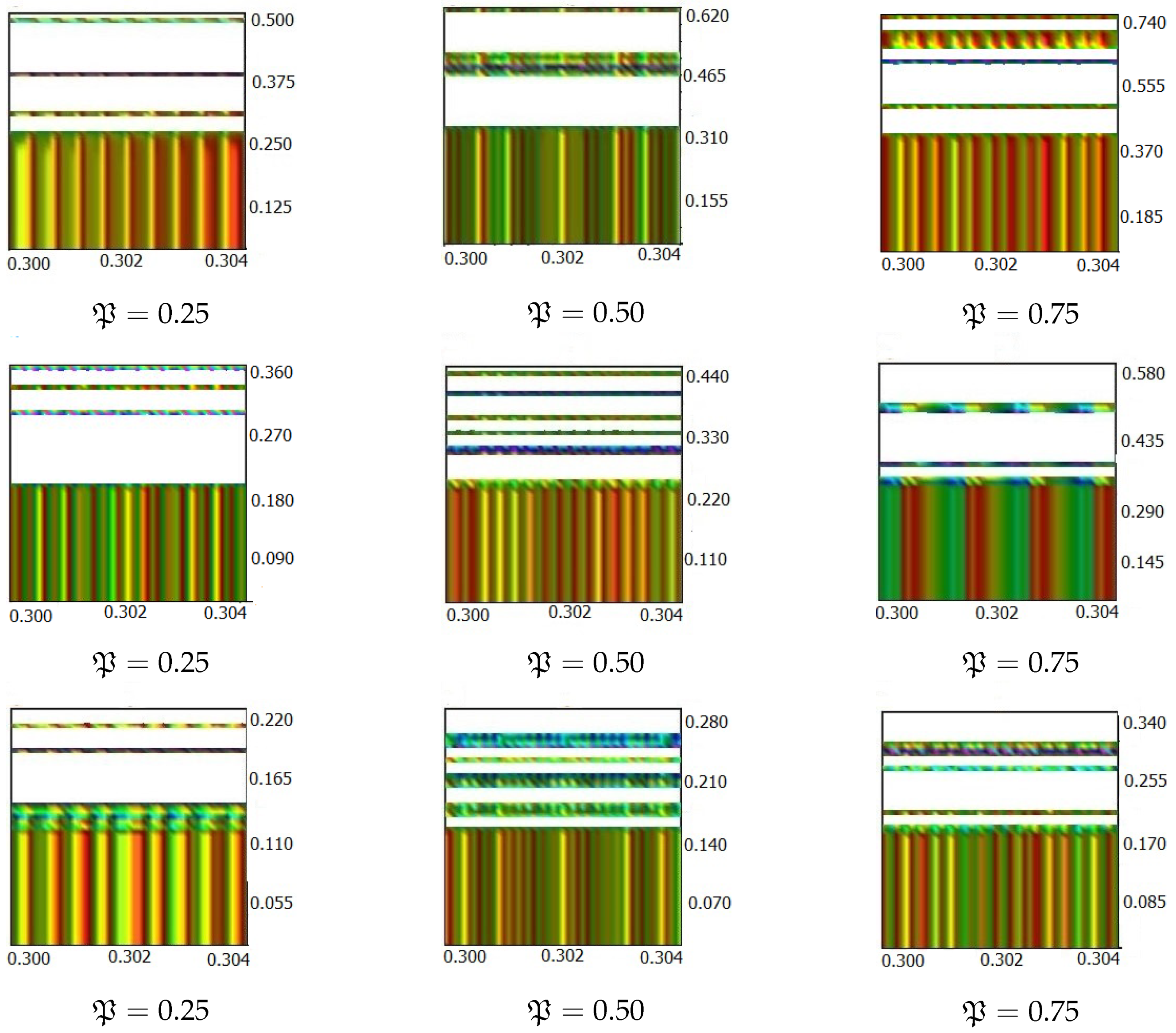
We present the contour plots of for in Figure 1, Figure 2, Figure 3 and Figure 4. In addition, we propose the contour plots of for and diverse values of in Figure 5. Contour lines are essential in mathematical modeling, as they provide a clear means of visualizing and analyzing complex surfaces and scalar fields. By representing points of equal value, they help identify patterns, trends, and critical regions in data without the need for 3D graphs. During optimization, they reveal gradients, minima, and maxima, thereby guiding algorithms such as gradient descent. In physics and engineering, they are used to model equipotential lines, pressure distributions, and temperature gradients. In geospatial applications they are employed as contour lines for terrain mapping and hazard prediction, while in statistics, they are used to illustrate probability densities and clustering. Their ability to simplify multidimensional problems into interpretable 2D plots makes them invaluable across scientific and computational disciplines.
In Figure 5, we systematically calculate the differences in the resulting error when using the Wright control function compared to other cases where the controllers are various special functions, as indicated. As observed, the error discrepancy is smaller when the controllers are modeled using Wright and hypergeometric functions compared to other configurations. This suggests that the choice of controller function has a significant impact on the stability of the solutions. Therefore, selecting an appropriate control function can be highly effective in optimizing various aspects of the problem, including minimizing error, enhancing stability, and ultimately identifying the optimal solution. To facilitate a clearer understanding and provide a more detailed description of the above content, we present Table 1, which displays the use of various special functions as control functions. This table illustrates the versatility and applicability of different mathematical tools in modeling and analyzing the proposed problem. By including these special functions, we offer a comprehensive comparison and highlight the effectiveness of each in capturing complex behaviors. This approach not only enhances the interpretability of the results but also provides valuable insights into how different functions can be leveraged to improve the accuracy and robustness of models used across diverse scenarios. For this purpose, we introduce the following notation:where , and is as defined in Section 2.5. The error values for various values of are presented in Table 1. By comparing the results across the two different ranges, it can be concluded that selecting hypergeometric functions, followed by Wright functions, as control functions yields better outcomes than using exponential or Mittag–Leffler functions as controllers. Special functions are indispensable tools in stability analyses and optimization, as they enable the expression of solutions to complex mathematical models that are otherwise difficult to manage. Their unique analytical properties allow for a more precise characterization of system behavior, particularly in the nonlinear and boundary value problems common in control theory. These functions contribute to the development of tighter stability bounds, enhance the accuracy of predictive models, and support the design of optimal control strategies. By capturing subtle dynamics that standard functions often overlook, special functions significantly broaden the analytical framework used for addressing challenging problems related to system stability and optimality.


