Optimizing Optical Fiber Communications: Bifurcation Analysis and Soliton Dynamics in the Quintic Kundu–Eckhaus Model

Abstract

This paper investigates the bifurcation dynamics and optical soliton solutions of the integrable quintic Kundu–Eckhaus (QKE) equation with an M-fractional derivative. By adding quintic nonlinearity and higher-order dispersion, this model expands on the nonlinear Schrödinger equation, which makes it especially applicable in explaining the propagation of high-power optical waves in fiber optics. To comprehend the behavior of the connected dynamical system, we categorize its equilibrium points, determine and analyze its Hamiltonian structure, and look at phase diagrams. Moreover, integrating along periodic trajectories yields soliton solutions. We achieve this by using the simplest equation approach and the modified extended Tanh method, which allow for a thorough investigation of soliton structures in the fractional QKE model. The model provides useful implications for reducing internet traffic congestion by including fractional temporal dynamics, which enables directed flow control to avoid bottlenecks. Periodic breather waves, bright and dark kinky periodic waves, periodic lump solitons, brilliant-dark double periodic waves, and multi-kink-shaped waves are among the several soliton solutions that are revealed by the analysis. The establishment of crucial parameter restrictions for soliton existence further demonstrates the usefulness of these solutions in optimizing optical communication systems. The theoretical results are confirmed by numerical simulations, highlighting their importance for practical uses.

1. Introduction

Nonlinear science has become a crucial domain for comprehending the cosmos as it elucidates the intriguing nonlinear phenomena present in nature. It is important to look into different nonlinear partial differential equations (NLPDEs) to describe complex systems that are quantitatively dynamic. Since the mid-18th century, scholars have concentrated on elucidating intricate physical processes for application in NLPDEs, hence enhancing the importance of this field of study. Scientists often use nonlinear differential models to study how nonlinear optical fibers work [1,2,3,4,5,6], to study how particles move in solid-state physics [3], how high-amplitude waves travel, to study fluid dynamics [7], bahavior of nanofluid [8], and how plasma behaves [9].

It is important to obtain analytical and accurate solutions to nonlinear models. Examining the solutions and properties of NLPDEs deepens our comprehension of their foundational structures. These work are all connected in a complex way by solitary wave theory, which shows how important soliton solution techniques are for solving NLEEs, including inverse scatting [10], generalized (G′/G)-expansion [11], the extended modified direct algebraic method [12], extended trial function [13], semi-inverse method [14], new extended direct algebraic method [15], enhanced direct algebraic approach [16], reliable expansion [17], modified Sardar sub equation [18], simplified Hirota bilinear method [19], simplified Hirota’s method [20], generalized Riccati equation mapping method [21], Nonlinearization technique [22], tri-Hamiltonian approach [23], imporved F-expansion method [24], MSE mthod [25], tanh and the extended tanh [26], Hirota bilinear [27], new MSE technique [28], nonlinearization method [29,30], eigenvalue variational method [31], next-generation matrix method [32], and Improved Modified Extended Tanh-Function technique [33].

Fiber optic technologies are the foundation of contemporary information technology, serving a crucial function in communication networks and internet infrastructure. Optical fiber communication methods have transformed long-distance data transfer by offering remarkable capacity and little signal loss. These developments facilitate the effortless transmission of information across extensive distances. Advancements in optical signal processing have enhanced the efficacy of all-optical communication systems. Active optical components allow control and transmission to work together in a single fiber, which has many benefits. These parts, which are made using fiber drawing methods, are not limited by the sizes of chip-based devices, which makes them useful for certain tasks like optical buffering. Because fiber optic equipment works with all-fiber reconfigurable networks, there is very little insertion loss during integration. Solitons are very useful in fiber optic systems because they keep their particle-like properties even when there are big changes, they are not affected by polarization modes or dispersion, and they can send data as optical bits by nature. The characteristics of solitons render them an ideal candidate for the development of efficient all-optical switching systems.

Fractional derivatives, which extend standard integer-order differentiation, have garnered considerable interest across multiple disciplines, including mathematics, physics, and engineering. When compared to normal derivatives, which show local rates of change, fractional derivatives allow us to include memory and genetic traits in complex systems [34]. This distinctive characteristic renders them appropriate for modeling anomalous diffusion, viscoelastic substances, and nonlinear wave processes [35]. The notion of fractional differentiation originated in the 17th century when Leibniz and L’Hôpital explored the feasibility of a derivative of non-integer order. Nonetheless, stringent mathematical formulations arose somewhat later, influenced by the contributions of Liouville, Riemann, and Caputo [36]. There are many ways to define fractional derivatives, such as the Riemann–Liouville, Caputo, and Grünwald–Letnikov derivatives, which are all designed for different purposes [37].

In recent years, fractional calculus has been widely utilized in nonlinear evolution equations, soliton theory, and optical physics. The nonlinear Schrödinger equation can be changed to fractional forms that help us understand how waves move in chaotic and dispersed environments [38]. Also, numerical and analytical methods like the Adomian decomposition and variational iteration approaches have been proven to work well with fractional differential equations [39].

This paper examines dynamical behavior through bifurcation analysis and the importance of fractional derivatives on the optical soliton solution of the M-fractional QKE equation through MEH and SE techniques and also focuses on how they affect the dynamics of soliton particles and the criteria for integrability. We provide a comparative analysis of M-fractional operators to clarify their role in regulating complex physical systems.

2. Governing Model

The quintic Kundu–Eckhaus (QKE) equation is a nonlinear evolution equation that describes how complicated optical waves move, especially when light with a lot of power moves through optical fibers. It adds to the nonlinear Schrödinger equation by including quintic nonlinearity and higher-order dispersion. This makes it necessary to study solitons, rogue waves, and modulational instability in nonlinear optical systems. The QKE equation controls how pulses move through optical fibers. It does this by using quintic terms to make soliton stability better and to handle nonlinear effects like self-phase modulation and energy transfer. It is very important to understand rogue waves, which are strong increases in optical turbulence, and modulational instability, which cause periodic waves to form. Higher-order dispersion effects also make pulse splitting and nonlinear wave mixing easier, which are important for making super continuums and making progress in fiber-optic communication. The QKE equation [40] gives us a way to look at and improve the patterns of light waves in fiber optics, laser–plasma interactions, and photonic systems. Its solutions make signal stability, pulse shaping, and nonlinear wave management better, which makes it an important tool for modern photonics and optical communication technologies.

$$i{D}_{M,t}^{\beta ,n}H\left(x,t\right)+A{\displaystyle \frac{{\partial }^{2}H\left(x,t\right)}{{\partial x}^2}}+B{\left|H\left(x,t\right)\right|}^{4}H\left(x,t\right)+E{\left({\left|H\left(x,t\right)\right|}^2\right)}_{x}H\left(x,t\right)=0.$$

(1)

Equation (1) is the time M-fractional QKE equation [36], where $D_{M,t}^{\beta ,n}$ is the M-fractional differential operator, and $H\left(x,t\right)$ is the dependent variable and denotes the soliton pulse profile and generally aligns with the envelope of the optical field. The initial term in Equation (1) delineates the temporal evolution of the nonlinear wave, whereas the term $A{\displaystyle \frac{{\partial }^{2}H\left(x,t\right)}{{\partial x}^2}}$ accounts for the spatial curvature of the wave profile, signifying dispersive effects within the medium. The nonlinear interaction of the wave is dictated by the expression $B{\left|H\left(x,t\right)\right|}^{4}H\left(x,t\right)$, where ${\left|H\left(x,t\right)\right|}^4$ denotes the wave intensity. Furthermore, the expression $E{\left({\left|H\left(x,t\right)\right|}^2\right)}_{x}H\left(x,t\right)$ includes the spatial derivative of the wave intensity ${\left|H\left(x,t\right)\right|}^2$, signifying higher-order dispersion effects or the impact of a nonlocal nonlinearity. The real-valued coefficients $A, B$, and $E$ pertain to group velocity dispersion, quintic nonlinearity, and associated physical phenomena. Now, we use a traveling wave variable as follows:

$$H\left(x,t\right)=H\left(\psi \right)e^{i\phi }; \psi =K\left(x-\omega {\displaystyle \frac{\mathsf{\Gamma }\left(n+1\right)}{\beta }}{t}^{\beta }\right), \phi =-px+v{\displaystyle \frac{\mathsf{\Gamma }\left(n+1\right)}{\beta }}{t}^{\beta }+\delta .$$

(2)

Where $H\left(\psi \right)$ is the amplitude of the wave, $e^{i\phi }$ is the phase term, $K$ is the scaling parameter influencing the shape of the traveling wave, $\omega$ is the velocity affecting the wave speed, $p$ is the wave number, $v$ is the phase velocity parameter, and $\delta$ is a phase constant.

Now, Equation (2) is inserted into Equation (1), and the real and imaginary portions are separated to yield

$$\mathrm{Real}: A{K}^2{H}^{″}-\left(v+A{p}^2\right)H+2EK{H}^2{H}^{\prime }+B{H}^5=0,$$

(3)

and imaginary: $\omega =-2Ap$.

If we balance $H^{″}$ and $H^5$, then we obtain $N={\displaystyle \frac{1}{2}}$. So, consider $H\left(\psi \right)=R^{{\displaystyle \frac{1}{2}}}$. If we insert $H\left(\psi \right)=R^{{\displaystyle \frac{1}{2}}}$ into Equation (3), then we obtain the following equation:

$$2A{K}^{2}R{R}^{″}+4EK{R}^2{R}^{\prime }-A{K}^2{\left(H^{\prime }\right)}^2-4\left(v+A{p}^2\right)R^2+4B{R}^4.$$

(4)

3. Dynamic Analysis

Equation (4) can be written into the following form:

$$H^{″}={\displaystyle \frac{\left(v+A{p}^2\right)}{A{K}^2}}H-{\displaystyle \frac{2EK}{A{K}^2}}{H}^2{H}^{\prime }-{\displaystyle \frac{B}{A{K}^2}}B{H}^5=0.$$

(5)

Now, we apply the Galilean Transformation to Equation (5), and we obtain the following system of equations:

$$\left.\begin{array}{c}{\displaystyle \frac{dH}{d\psi }}=G\\ {\displaystyle \frac{dG}{d\psi }}={\chi }_1{H}^{2}G+{\chi }_2{H}^5+{\chi }_{3}H\end{array}\right\}.$$

(6)

Where ${\chi }_1=-{\displaystyle \frac{2EK}{A{K}^2}}, {\chi }_2=-{\displaystyle \frac{B}{A{K}^2}}, \mathrm{a}\mathrm{n}\mathrm{d} {\chi }_3={\displaystyle \frac{\left(v+A{p}^2\right)}{A{K}^2}}$.

Now, we explain the diverse phenomena of the system in Equation (6) by using bifurcation theory. The bifurcation theory plays a vital role in exploring the behavior of the system shown in Equation (6). The $H\left(\phi \right)$ has continuous solutions of Equation (5) for $\psi \in \mathbb{R}$ with $\underset{\psi \to +\infty }{\lim }H\left(\psi \right)=a$ and $\underset{\psi \to -\infty }{\lim }H\left(\psi \right)=b$. Wave function $H\left(\psi \right)$ represents solitary wave phenomena if $a=b$ and $H\left(\delta \right)$ represents kink wave (anti-kink) phenomena if $a\ne b$. In general, the homoclinic orbit represents solitary wave solutions, and the heteroclinic orbit represents kink or anti-kink phenomena for the system shown in Equation (6). From Equation (6), for equilibrium points,

$$\left.\begin{array}{c}G=0\\ {\chi }_1{H}^{2}G+{\chi }_2{H}^5+{\chi }_{3}H=0\end{array}\right\}.$$

(7)

By solving the system in Equation (7), we obtain

$$N_0=\left(\mathrm{0,0}\right), N_1=\left(0,-\sqrt[4]{-{\displaystyle \frac{{\chi }_2}{{\chi }_3}}}\right), N_2=\left(0, \sqrt[4]{-{\displaystyle \frac{{\chi }_2}{{\chi }_3}}}\right).$$

$$J_N=\left(\begin{array}{cc}0& 1\\ 2{\chi }_{1}HG+5{\chi }_2{H}^4+{\chi }_3& {\chi }_1{H}^2\end{array}\right),$$

$$D\left(e\right)=-\left(-C_1{\displaystyle \frac{{G_e}^2}{{M_e}^2}}+C_2+C_3{M}_e\right).$$

According to the theory of planar, the observations are as follows: If $D\left(e\right)<0$, then $e$ is the point of the saddle. If $D\left(e\right)>0$ and $T\left(e\right)=0$, then point $e$ is the center point. If $D\left(e\right)=0$, then $e$ is the cup’s point.

• Case 1: for ${\displaystyle \frac{{\chi }_2}{{\chi }_3}}>0$.

• Subcase 1.1: For ${\chi }_1>0, {\chi }_2>0, {\chi }_3>0$.

In Figure 1, the trajectories are not closed at the point $N_0=\left(\mathrm{0,0}\right)$. So, the point $N_0=\left(\mathrm{0,0}\right)$ is a saddle point and unstable.

• Subcase 1.2: For ${\chi }_1>0, {\chi }_2<0, {\chi }_3<0$.

In Figure 2, the trajectories are not closed at the point $N_0=\left(\mathrm{0,0}\right)$. So, the point $N_0=\left(\mathrm{0,0}\right)$ is a saddle point and unstable.

• Case 2: for ${\displaystyle \frac{{\chi }_2}{{\chi }_3}}>0$.

• Subcase 2.1: For ${\chi }_1>0, {\chi }_2<0, {\chi }_3>0$.

In Figure 3, the trajectories are not closed at the point $N_0=\left(\mathrm{0,0}\right)$. So, the point $N_0=\left(\mathrm{0,0}\right)$ is a saddle point and unstable. The trajectories are closed at the points $N_1=\left(0,-\sqrt[4]{-{\displaystyle \frac{{\chi }_2}{{\chi }_3}}}\right)$ and $N_2=\left(0, \sqrt[4]{-{\displaystyle \frac{{\chi }_2}{{\chi }_3}}}\right)$. So, these points are center points and stable.

• Subcase 2.2: For ${\chi }_1<0, {\chi }_2<0, {\chi }_3>0$.

In Figure 4, the trajectories are not closed at the point $N_0=\left(\mathrm{0,0}\right)$. So, the point $N_0=\left(\mathrm{0,0}\right)$ is a saddle point and unstable. The trajectories are closed at the points $N_1=\left(0,-\sqrt[4]{-{\displaystyle \frac{{\chi }_2}{{\chi }_3}}}\right)$ and $N_2=\left(0, \sqrt[4]{-{\displaystyle \frac{{\chi }_2}{{\chi }_3}}}\right)$. So, these points are center points and stable.

• Subcase 2.3: For ${\chi }_1>0, {\chi }_2>0, {\chi }_3<0$.

In Figure 5, the trajectories are closed at the point $N_0=\left(\mathrm{0,0}\right)$. So, the point $N_0=\left(\mathrm{0,0}\right)$ is a center point and stable. The trajectories are not closed at the points $N_1=\left(0,-\sqrt[4]{-{\displaystyle \frac{{\chi }_2}{{\chi }_3}}}\right)$, and $N_2=\left(0, \sqrt[4]{-{\displaystyle \frac{{\chi }_2}{{\chi }_3}}}\right)$. So, these points are saddle points and unstable.

• Subcase 2.4: For ${\chi }_1<0, {\chi }_2>0, {\chi }_3<0$.

In Figure 6, the trajectories are closed at the point $N_0=\left(\mathrm{0,0}\right)$. So, the point $N_0=\left(\mathrm{0,0}\right)$ is a center point and stable. The trajectories are not closed at the points $N_1=\left(0,-\sqrt[4]{-{\displaystyle \frac{{\chi }_2}{{\chi }_3}}}\right)$, and $N_2=\left(0, \sqrt[4]{-{\displaystyle \frac{{\chi }_2}{{\chi }_3}}}\right)$. So, these points are saddle points and unstable.

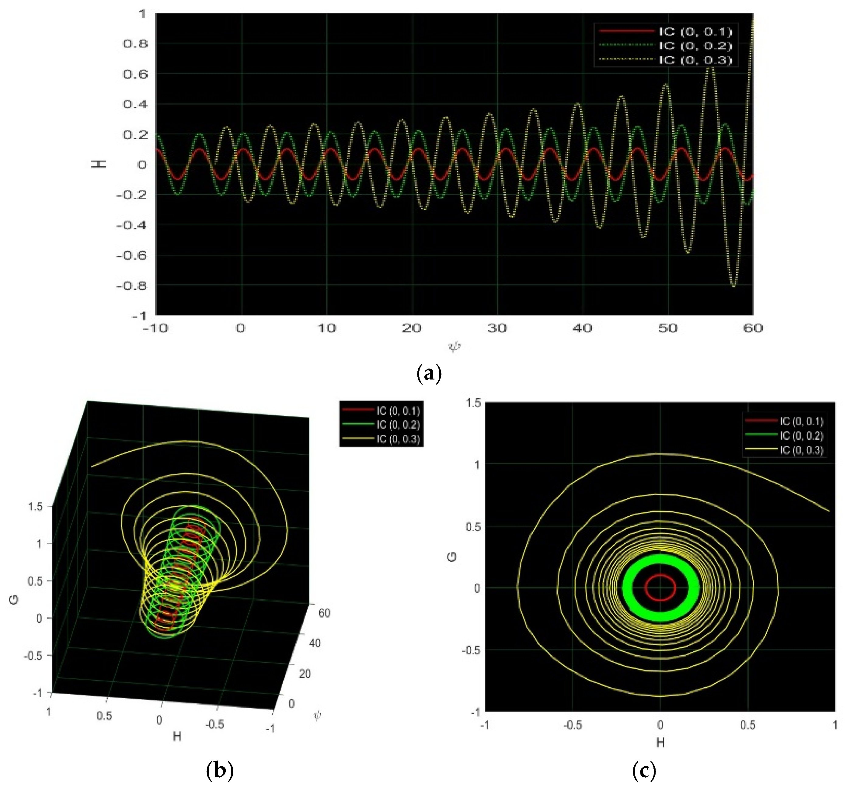
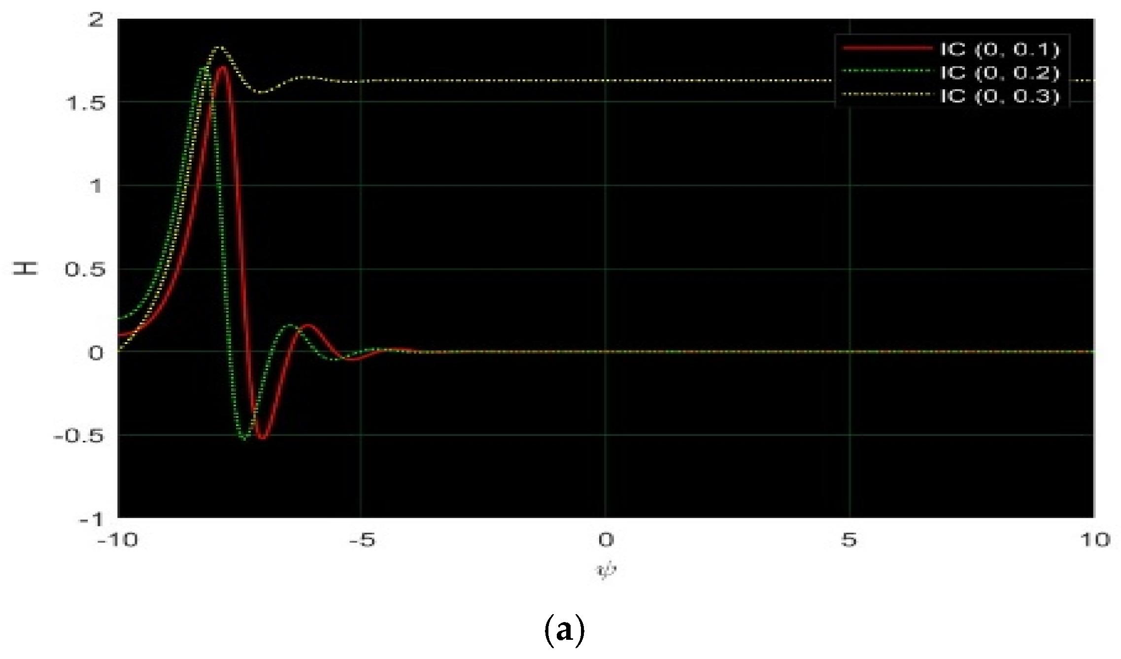
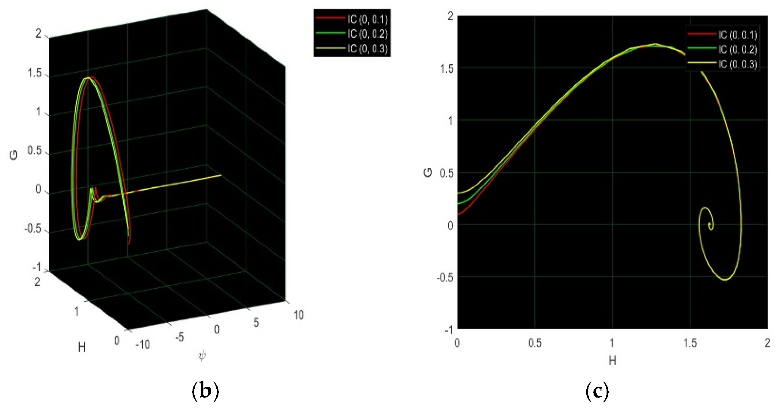
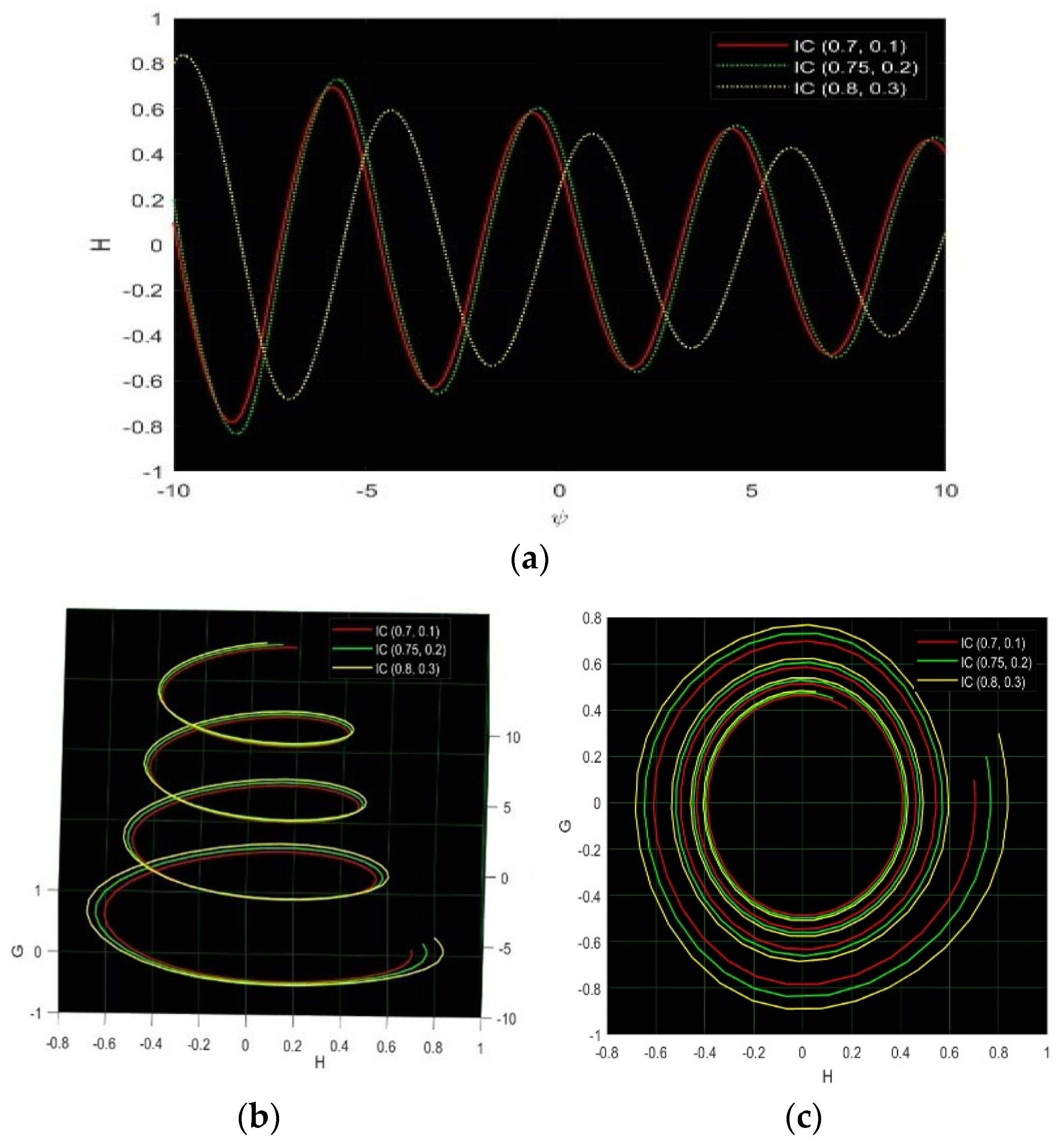
4. Sensitivity and Damping Effect

Numerical solutions with designated initial conditions can be derived using MATLAB-2023 utilizing the fourth-order Runge–Kutta method. This study investigates the influence of the dispersive coefficient, represented as A, which functions as a damping factor in the ordinary differential equation. As $A \to 0$ with $A \ne 0$, the wave structure demonstrates heightened oscillations (see Figure 7a–c). As $A$ grows over time $\left(\psi \right)$, these oscillations are progressively reduced (refer to Figure 7a–c). Furthermore, velocity $\left(v\right)$ affects motion in the presence of $A$, resulting in asymptotic instability, asymptotic stability, or perhaps neutralizing the damping effect. When $v$ is positive, it triggers phase transitions at the critical point and progressively enhances aperiodic circulations, finally leading to an asymptotically unstable state (Figure 8a–c). In contrast, negative values of $v$ lead to an asymptotically stable state, wherein the system gradually converges to the critical point over time (Figure 9a–c). Significantly, for elevated values of $v$, relative to $A$, the periodic orbits maintain proximity to the critical point, yielding a periodic solution (Figure 10a–c).

5. Methodology

This section explains the procedure of two efficient techniques, the modified extended Tanh and simplest equation methods, to solve NLEES. For this purpose, consider NLEEs as

$$L\left(H_t,H{H}_x, H_{xxx}, H_{tx} \right)=0.$$

(8)

Consider the transformation variable $\psi =Kx-vt; H\left(x,t\right)=H\left(\psi \right)$ to convert Equation (8) as follows:

$$L\left(-v{H}_{\psi },KH{H}_{\psi }, K^3 H_{\psi \psi \psi }, -vK H_{\psi \psi } \right)=0.$$

(9)

5.1. Fundamental Stage of Modified Extended Tanh Method [41]

The solution of Equation (9) is

$$H\left(\psi \right)={\beta }_0+{\sum }_{q=1}^s\left({\beta }_q{\mathrm{F}}^q\left(\psi \right)+{\displaystyle \frac{{\delta }_q}{{\mathrm{F}}^q\left(\psi \right)}}\right).$$

(10)

The function $\mathrm{F}\left(\psi \right)$ satisfied Equation (10):

$${\displaystyle \frac{dF\left(\psi \right)}{d\psi }}=\mathsf{\Theta }+F^2\left(\psi \right).$$

(11)

By inserting Equations (10) and (11) into Equation (9), we obtain the values of ${\beta }_q$, ${\delta }_s$, $K, and v$. We can insert these obtained values into Equation (10) and find the required solutions.

The solutions of Equation (11) are

• For $\mathsf{\Theta }<0,$

$$F\left(\psi \right)=-\sqrt{-\mathsf{\Theta }} tanh\left(\sqrt{-\mathsf{\Theta }}\left(\mathsf{\psi }+{\mathsf{\psi }}_0\right)\right), or F\left(\psi \right)=-\sqrt{-\mathsf{\Theta }} coth\left(\sqrt{-\mathsf{\Theta }}\left(\mathsf{\psi }+{\mathsf{\psi }}_0\right)\right).$$

For $\mathsf{\Theta }<0,$

$$F\left(\psi \right)=\sqrt{\mathsf{\Theta }}tan\left(\sqrt{\mathsf{\Theta }}\left(\mathsf{\psi }+{\mathsf{\psi }}_0\right)\right), or F\left(\psi \right)=-\sqrt{\mathsf{\Theta }}cot\left(\sqrt{\mathsf{\Theta }}\left(\mathsf{\psi }+{\mathsf{\psi }}_0\right)\right).$$

For $\mathsf{\Theta }=0$,

$$F\left(\psi \right)={\displaystyle \frac{1}{\mathsf{\psi }+{\mathsf{\psi }}_0}}.$$

5.2. Fundamental Stage of Simplest Equation Method [42,43]

Consider the trial solution of Equation (9) in the following:

$$H\left(\psi \right)={\beta }_0+{\sum }_{g=1}^m\left[{\beta }_g{F\left(\psi \right)}^g\right].$$

(12)

The wave function $F\left(\psi \right)$ in Equation (12) satisfied a subsequent differential equation:

$$F^{\prime }\left(\psi \right)={\Theta }_{1}F\left(\psi \right)+{\Theta }_2{F}^2\left(\psi \right).$$

(13)

By inserting Equations (12) and (13) into Equation (9), we obtain the values of ${\beta }_{\mathrm{g}}, {\mathsf{\beta }}_0$, $K, and v$. We can insert these obtained values into Equation (12) and find the required solutions.

The solutions of Equation (13) are

$$\begin{gathered} F\left(\psi \right)={\displaystyle \frac{{\Theta }_1{e}^{{\Theta }_1(\psi +{\psi }_0)}}{1-{\Theta }_2{e}^{{\Theta }_1(\psi +{\psi }_0)}}}; {\Theta }_2<0, {\Theta }_1>0. \\ and F\left(\psi \right)={\displaystyle \frac{-{\Theta }_1{e}^{{\Theta }_1(\psi +{\psi }_0)}}{1+{\Theta }_2{e}^{{\Theta }_1(\psi +{\psi }_0)}}}; {\Theta }_2>0, {\Theta }_1<0. \end{gathered}$$

If we set ${\mathsf{\Theta }}_2=-1$, Equation (9) is

$$F^{\prime }\left(\psi \right)={\mathsf{\Theta }}_{1}F\left(\psi \right)-F^2\left(\psi \right).$$

The solutions are

$$\begin{gathered} F\left(\psi \right)={\displaystyle \frac{{\Theta }_1}{2}}\left[1+\mathit{tanh}\left({\displaystyle \frac{{\Theta }_1}{2}}\left(\psi +{\psi }_0\right)\right)\right];{\Theta }_1>0. \\ F\left(\psi \right)={\displaystyle \frac{{\Theta }_1}{2}}\left[1-\mathit{coth}\left({\displaystyle \frac{{\Theta }_1}{2}}\left(\psi +{\psi }_0\right)\right)\right];{\Theta }_1<0. \end{gathered}$$

6. Optical Soliton Solutions of Quintic M-Fractional Kundu–Eckhaus Equation

In this section, we solve the quintic M-fractional Kundu–Eckhaus equation by using the modified extended Tanh method and the simplest equation method.

6.1. Application of the Modified Extended Tanh Method

In this subsection, we apply the modified extended Tanh method to solve the quintic M-fractional Kundu–Eckhaus equation. The balance number of Equation (4) is $s=1$. So, the solution of Equation (4) is

$$H\left(\psi \right)={\beta }_0+{\beta }_{1}F\left(\psi \right)+{\displaystyle \frac{{\delta }_1}{F\left(\psi \right)}}.$$

(14)

Equation (14) is substituted into Equation (4) along with Equation (11), and we can obtain the following solution sets:

$$\begin{gathered} K=\sqrt{{\displaystyle \frac{1}{4AE}}}B, v=-{\displaystyle \frac{4A{p}^{2}E+B^2\mathsf{\Theta }}{4E}}, {\beta }_0={\displaystyle \frac{B\sqrt{-\mathsf{\Theta }}}{4E}}, {\beta }_0=0, {\delta }_1={\displaystyle \frac{B\mathsf{\Theta }}{4E}}. \\ K=\sqrt{{\displaystyle \frac{1}{4AE}}}B, p=\sqrt{-{\displaystyle \frac{B^2\Theta +4Ev}{4AE}}}, {\beta }_0={\displaystyle \frac{B\sqrt{-\mathsf{\Theta }}}{4E}}, {\beta }_0=0, {\delta }_1={\displaystyle \frac{B\mathsf{\Theta }}{4E}}. \end{gathered}$$

Set-01: $K=\sqrt{{\displaystyle \frac{1}{4AE}}}B, v=-{\displaystyle \frac{4A{p}^{2}E+B^2\mathsf{\Theta }}{4E}}, {\beta }_0={\displaystyle \frac{B\sqrt{-\mathsf{\Theta }}}{4E}}, {\beta }_0=0, {\delta }_1={\displaystyle \frac{B\mathsf{\Theta }}{4E}}.$ For $\mathsf{\Theta }<0,$

$$H\left(x,t\right)={\left({\displaystyle \frac{B\sqrt{-\mathsf{\Theta }}}{4E}}-{\displaystyle \frac{\frac{B\mathsf{\Theta }}{4E}}{\sqrt{-\vartheta }tanh\left(\sqrt{-\vartheta }\left(\mathsf{\psi }+{\mathsf{\psi }}_0\right)\right)}}\right)}^{{\displaystyle \frac{1}{2}}}{e}^{i\phi }.$$

(15)

$$H\left(x,t\right)={\left({\displaystyle \frac{B\sqrt{-\mathsf{\Theta }}}{4E}}-{\displaystyle \frac{\frac{B\mathsf{\Theta }}{4E}}{\sqrt{-\vartheta }coth\left(\sqrt{-\vartheta }\left(\mathsf{\psi }+{\mathsf{\psi }}_0\right)\right)}}\right)}^{{\displaystyle \frac{1}{2}}}{e}^{i\phi }.$$

(16)

For $\mathsf{\Theta }<0,$

$$H\left(x,t\right)={\left({\displaystyle \frac{B\sqrt{-\mathsf{\Theta }}}{4E}}+{\displaystyle \frac{\frac{B\mathsf{\Theta }}{4E}}{\sqrt{\vartheta }tan\left(\sqrt{\vartheta }\left(\mathsf{\psi }+{\mathsf{\psi }}_0\right)\right)}}\right)}^{{\displaystyle \frac{1}{2}}}{e}^{i\phi }.$$

(17)

$$H\left(x,t\right)={\left({\displaystyle \frac{B\sqrt{-\mathsf{\Theta }}}{4E}}-{\displaystyle \frac{\frac{B\mathsf{\Theta }}{4E}}{\sqrt{\vartheta }cot\left(\sqrt{\vartheta }\left(\mathsf{\psi }+{\mathsf{\psi }}_0\right)\right)}}\right)}^{{\displaystyle \frac{1}{2}}}{e}^{i\phi }.$$

(18)

Here, $\psi =\sqrt{{\displaystyle \frac{1}{4AE}}}B\left(x+2Ap{\displaystyle \frac{\mathsf{\Gamma }\left(n+1\right)}{\beta }}{t}^{\beta }\right), \phi =-px-{\displaystyle \frac{4A{p}^{2}E+B^2\mathsf{\Theta }}{4E}}{\displaystyle \frac{\mathsf{\Gamma }\left(n+1\right)}{\beta }}{t}^{\beta }+\delta$.

• Set-02: $K=\sqrt{{\displaystyle \frac{1}{4AE}}}B, p=\sqrt{-{\displaystyle \frac{B^2\mathsf{\Theta }+4\mathrm{E}\mathrm{v}}{4AE}}}, {\beta }_0={\displaystyle \frac{B\sqrt{-\mathsf{\Theta }}}{4E}}, {\beta }_0=0, {\delta }_1={\displaystyle \frac{B\mathsf{\Theta }}{4E}}.$

• For $\mathsf{\Theta }<0,$

$$H\left(x,t\right)={\left({\displaystyle \frac{B\sqrt{-\mathsf{\Theta }}}{4E}}-{\displaystyle \frac{B\mathsf{\Theta }}{4E}}\sqrt{-\vartheta }tanh\left(\sqrt{-\vartheta }\left(\mathsf{\psi }+{\mathsf{\psi }}_0\right)\right)\right)}^{{\displaystyle \frac{1}{2}}}{e}^{i\phi }.$$

(19)

$$H\left(x,t\right)={\left({\displaystyle \frac{B\sqrt{-\mathsf{\Theta }}}{4E}}-{\displaystyle \frac{B\mathsf{\Theta }}{4E}}\sqrt{-\vartheta }coth\left(\sqrt{-\vartheta }\left(\mathsf{\psi }+{\mathsf{\psi }}_0\right)\right)\right)}^{{\displaystyle \frac{1}{2}}}{e}^{i\phi }.$$

(20)

For $\mathsf{\Theta }<0,$

$$H\left(x,t\right)={\left({\displaystyle \frac{B\sqrt{-\mathsf{\Theta }}}{4E}}+{\displaystyle \frac{B\mathsf{\Theta }}{4E}}\sqrt{\vartheta }tan\left(\sqrt{\vartheta }\left(\mathsf{\psi }+{\mathsf{\psi }}_0\right)\right)\right)}^{{\displaystyle \frac{1}{2}}}{e}^{i\phi }.$$

(21)

$$H\left(x,t\right)={\left({\displaystyle \frac{B\sqrt{-\mathsf{\Theta }}}{4E}}-{\displaystyle \frac{B\mathsf{\Theta }}{4E}}\sqrt{\vartheta }cot\left(\sqrt{\vartheta }\left(\mathsf{\psi }+{\mathsf{\psi }}_0\right)\right)\right)}^{{\displaystyle \frac{1}{2}}}{e}^{i\phi }.$$

(22)

Here, $\psi =\sqrt{{\displaystyle \frac{1}{4AE}}}B\left(x+2Ap{\displaystyle \frac{\mathsf{\Gamma }\left(n+1\right)}{\beta }}{t}^{\beta }\right), \phi =-\sqrt{-{\displaystyle \frac{B^2\mathsf{\Theta }+4\mathrm{E}\mathrm{v}}{4AE}}}x+v{\displaystyle \frac{\mathsf{\Gamma }\left(n+1\right)}{\beta }}{t}^{\beta }+\delta$.

6.2. Application of the Simplest Equation Method

In this subsection, we apply the simplest equation method to solve the quintic M-fractional Kundu–Eckhaus equation. The balance number of Equation (4) is $N=1$. So, the solution of Equation (4) is

$$H\left(\psi \right)={\beta }_0+{\beta }_{1}F\left(\psi \right).$$

(23)

Equation (23) is substituted into Equation (4) along with Equation (13), and we obtain the following solution sets:

$$\begin{gathered} K=\sqrt{{\displaystyle \frac{1}{4AE}}}B, v={\displaystyle \frac{B^2{\mathsf{\Theta }}_1^2-16\mathrm{E}\mathrm{A}{p}^2}{16AE}}, {\beta }_0=-{\displaystyle \frac{B{\mathsf{\Theta }}_1}{4E}}, {\beta }_1=-{\displaystyle \frac{B{\mathsf{\Theta }}_2}{4E}}. \\ K=\sqrt{{\displaystyle \frac{1}{4AE}}}B, p=\sqrt{-{\displaystyle \frac{-B^2{\mathsf{\Theta }}_1^2+16\mathrm{E}\mathrm{v}}{16AE}}}, {\beta }_0=-{\displaystyle \frac{B{\mathsf{\Theta }}_1}{4E}}, {\beta }_1=-{\displaystyle \frac{B{\mathsf{\Theta }}_2}{4E}}. \end{gathered}$$

• Set-01: $K=\sqrt{{\displaystyle \frac{1}{4AE}}}B, v={\displaystyle \frac{B^2{\mathsf{\Theta }}_1^2-16\mathrm{E}\mathrm{A}{p}^2}{16AE}}, {\beta }_0=-{\displaystyle \frac{B{\mathsf{\Theta }}_1}{4E}}, {\beta }_1=-{\displaystyle \frac{B{\mathsf{\Theta }}_2}{4E}}$.

$$H\left(x,t\right)={\left(-{\displaystyle \frac{B{\mathsf{\Theta }}_1}{4E}}-{\displaystyle \frac{B{\mathsf{\Theta }}_2}{4E}}{\displaystyle \frac{{\mathsf{\Theta }}_1{e}^{{\mathsf{\Theta }}_1(\mathsf{\psi }+{\mathsf{\psi }}_0)}}{1-{\mathsf{\Theta }}_2{e}^{{\mathsf{\Theta }}_1(\mathsf{\psi }+{\mathsf{\psi }}_0)}}}\right)}^{{\displaystyle \frac{1}{2}}}{e}^{i\phi }; {\mathsf{\Theta }}_2<0, {\mathsf{\Theta }}_1>0.$$

(24)

$$H\left(x,t\right)={\left(-{\displaystyle \frac{B{\mathsf{\Theta }}_1}{4E}}-{\displaystyle \frac{B{\mathsf{\Theta }}_2}{4E}}{\displaystyle \frac{-{\mathsf{\Theta }}_1{e}^{{\mathsf{\Theta }}_1(\psi +{\psi }_0)}}{1+{\mathsf{\Theta }}_2{e}^{{\mathsf{\Theta }}_1(\psi +{\psi }_0)}}}\right)}^{{\displaystyle \frac{1}{2}}}{e}^{i\phi };{\mathsf{\Theta }}_2>0, {\mathsf{\Theta }}_1<0.$$

(25)

$$H\left(x,t\right)={\left(-{\displaystyle \frac{B{\mathsf{\Theta }}_1}{4E}}-{\displaystyle \frac{B{\mathsf{\Theta }}_2}{4E}}{\displaystyle \frac{{\mathsf{\Theta }}_1}{2}}\left[1+\tanh \left({\displaystyle \frac{{\mathsf{\Theta }}_1}{2}}\left(\mathsf{\psi }+{\mathsf{\psi }}_0\right)\right)\right]\right)}^{{\displaystyle \frac{1}{2}}}{e}^{i\phi };{\mathsf{\Theta }}_1>0.$$

(26)

$$H\left(x,t\right)={\left(-{\displaystyle \frac{B{\mathsf{\Theta }}_1}{4E}}-{\displaystyle \frac{B{\mathsf{\Theta }}_2}{4E}}{\displaystyle \frac{{\mathsf{\Theta }}_1}{2}}\left[1-\coth \left({\displaystyle \frac{{\mathsf{\Theta }}_1}{2}}\left(\mathsf{\psi }+{\mathsf{\psi }}_0\right)\right)\right]\right)}^{{\displaystyle \frac{1}{2}}}{e}^{i\phi };{\mathsf{\Theta }}_1<0.$$

(27)

Here, $\psi =\sqrt{{\displaystyle \frac{1}{4AE}}}B\left(x+2Ap{\displaystyle \frac{\mathsf{\Gamma }\left(n+1\right)}{\beta }}{t}^{\beta }\right), \phi =-px-{\displaystyle \frac{4A{p}^{2}E+B^2\mathsf{\Theta }}{4E}}{\displaystyle \frac{\mathsf{\Gamma }\left(n+1\right)}{\beta }}{t}^{\beta }+\delta$.

• Set-02: $K=\sqrt{{\displaystyle \frac{1}{4AE}}}B, p=\sqrt{-{\displaystyle \frac{-B^2{\mathsf{\Theta }}_1^2+16\mathrm{E}\mathrm{v}}{16AE}}}, {\beta }_0=-{\displaystyle \frac{B{\mathsf{\Theta }}_1}{4E}}, {\beta }_1=-{\displaystyle \frac{B{\mathsf{\Theta }}_2}{4E}}$.

$$H\left(x,t\right)={\left(-{\displaystyle \frac{B{\mathsf{\Theta }}_1}{4E}}-{\displaystyle \frac{B{\mathsf{\Theta }}_2}{4E}}{\displaystyle \frac{{\mathsf{\Theta }}_1{e}^{{\mathsf{\Theta }}_1(\mathsf{\psi }+{\mathsf{\psi }}_0)}}{1-{\mathsf{\Theta }}_2{e}^{{\mathsf{\Theta }}_1(\mathsf{\psi }+{\mathsf{\psi }}_0)}}}\right)}^{{\displaystyle \frac{1}{2}}}{e}^{i\phi }; {\mathsf{\Theta }}_2<0, {\mathsf{\Theta }}_1>0.$$

(28)

$$H\left(x,t\right)={\left(-{\displaystyle \frac{B{\mathsf{\Theta }}_1}{4E}}-{\displaystyle \frac{B{\mathsf{\Theta }}_2}{4E}}{\displaystyle \frac{-{\mathsf{\Theta }}_1{e}^{{\mathsf{\Theta }}_1(\psi +{\psi }_0)}}{1+{\mathsf{\Theta }}_2{e}^{{\mathsf{\Theta }}_1(\psi +{\psi }_0)}}}\right)}^{{\displaystyle \frac{1}{2}}}{e}^{i\phi };{\mathsf{\Theta }}_2>0, {\mathsf{\Theta }}_1<0.$$

(29)

$$H\left(x,t\right)={\left(-{\displaystyle \frac{B{\mathsf{\Theta }}_1}{4E}}-{\displaystyle \frac{B{\mathsf{\Theta }}_2}{4E}}{\displaystyle \frac{{\mathsf{\Theta }}_1}{2}}\left[1+\tanh \left({\displaystyle \frac{{\mathsf{\Theta }}_1}{2}}\left(\mathsf{\psi }+{\mathsf{\psi }}_0\right)\right)\right]\right)}^{{\displaystyle \frac{1}{2}}}{e}^{i\phi };{\mathsf{\Theta }}_1>0.$$

(30)

$$H\left(x,t\right)={\left(-{\displaystyle \frac{B{\mathsf{\Theta }}_1}{4E}}-{\displaystyle \frac{B{\mathsf{\Theta }}_2}{4E}}{\displaystyle \frac{{\mathsf{\Theta }}_1}{2}}\left[1-\coth \left({\displaystyle \frac{{\mathsf{\Theta }}_1}{2}}\left(\mathsf{\psi }+{\mathsf{\psi }}_0\right)\right)\right]\right)}^{{\displaystyle \frac{1}{2}}}{e}^{i\phi };{\mathsf{\Theta }}_1<0.$$

(31)

Here, $\psi =\sqrt{{\displaystyle \frac{1}{4AE}}}B\left(x+2Ap{\displaystyle \frac{\mathsf{\Gamma }\left(n+1\right)}{\beta }}{t}^{\beta }\right), \phi =-px-{\displaystyle \frac{4A{p}^{2}E+B^2\mathsf{\Theta }}{4E}}{\displaystyle \frac{\mathsf{\Gamma }\left(n+1\right)}{\beta }}{t}^{\beta }+\delta$.

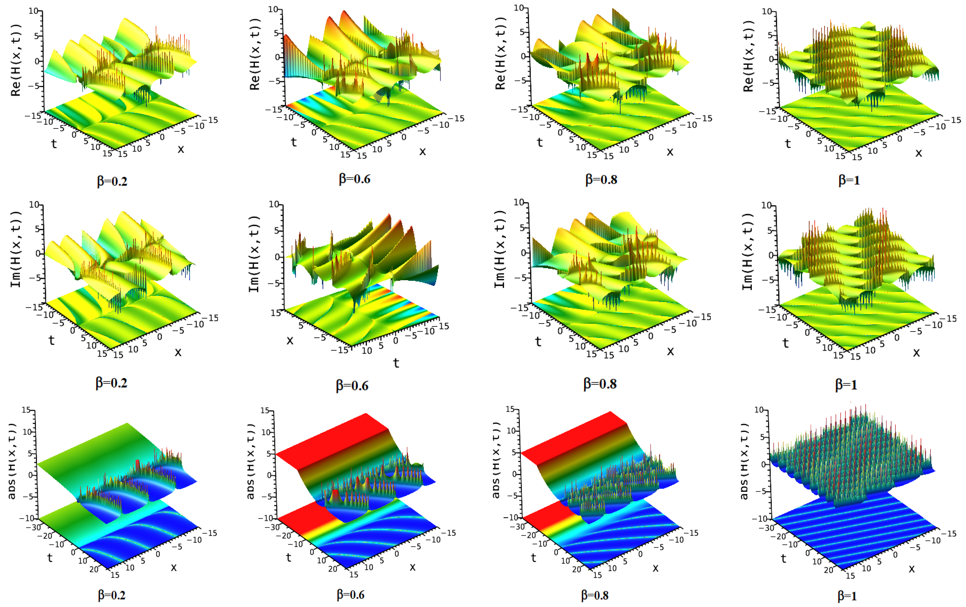
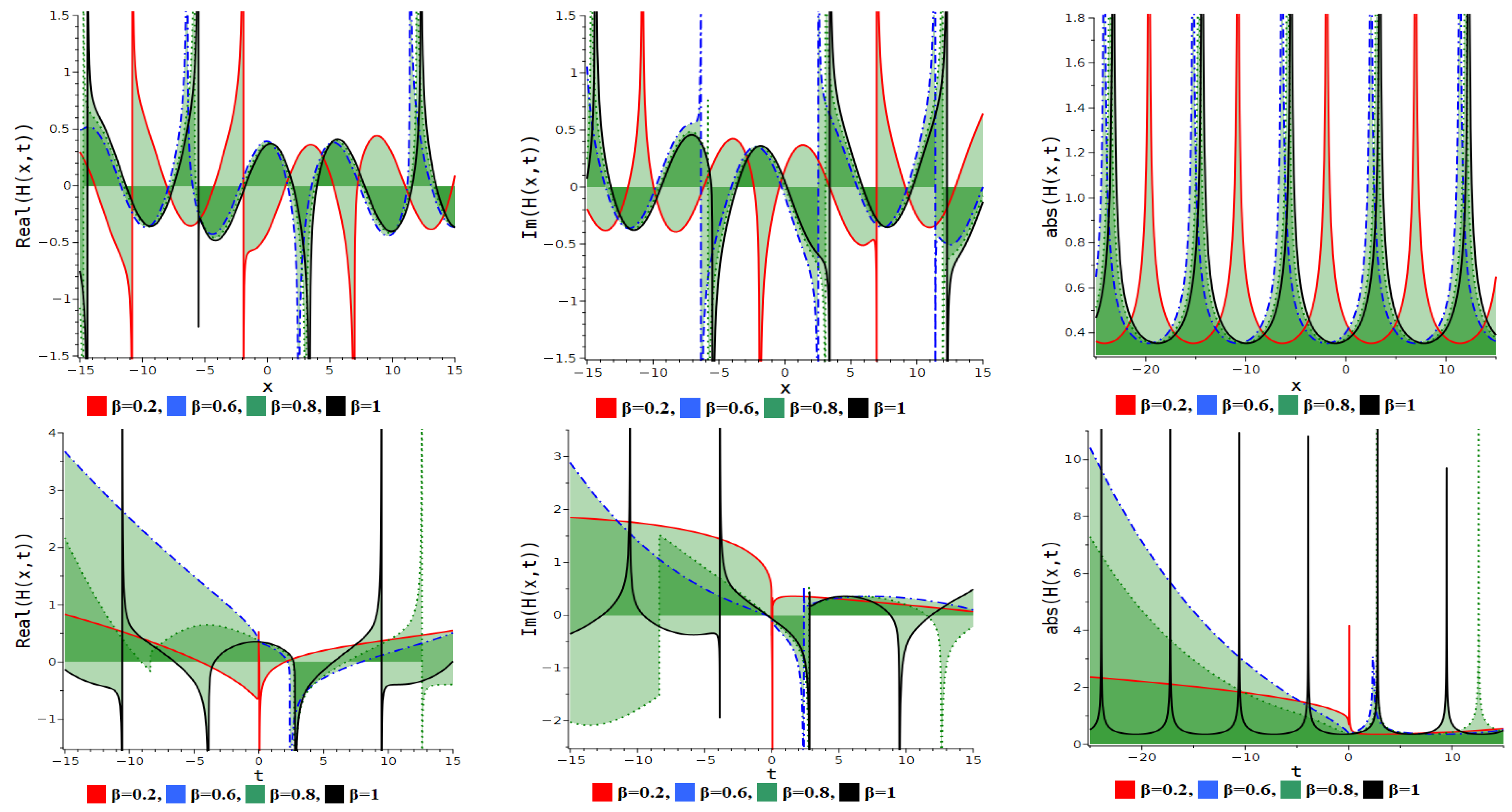
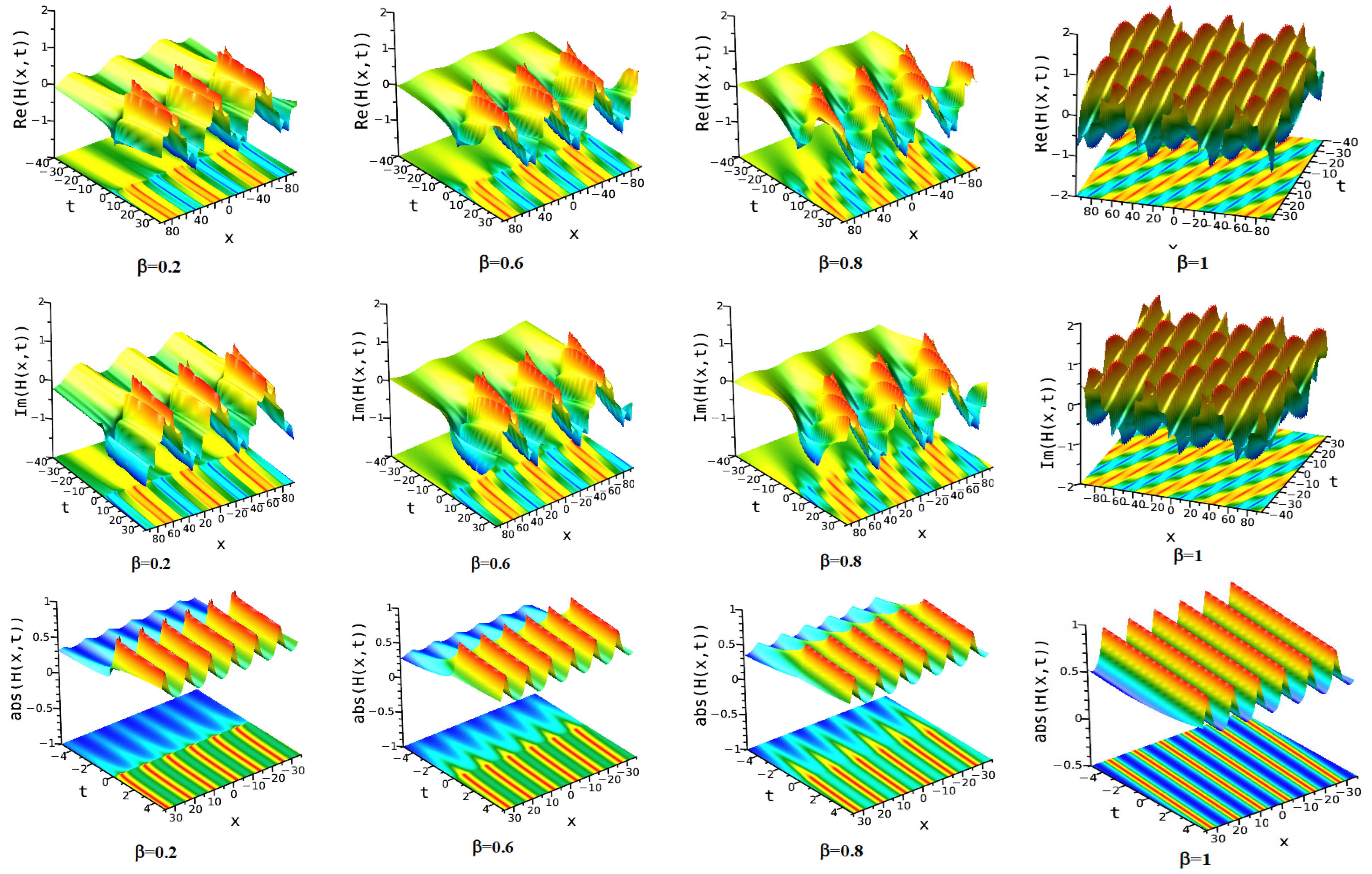
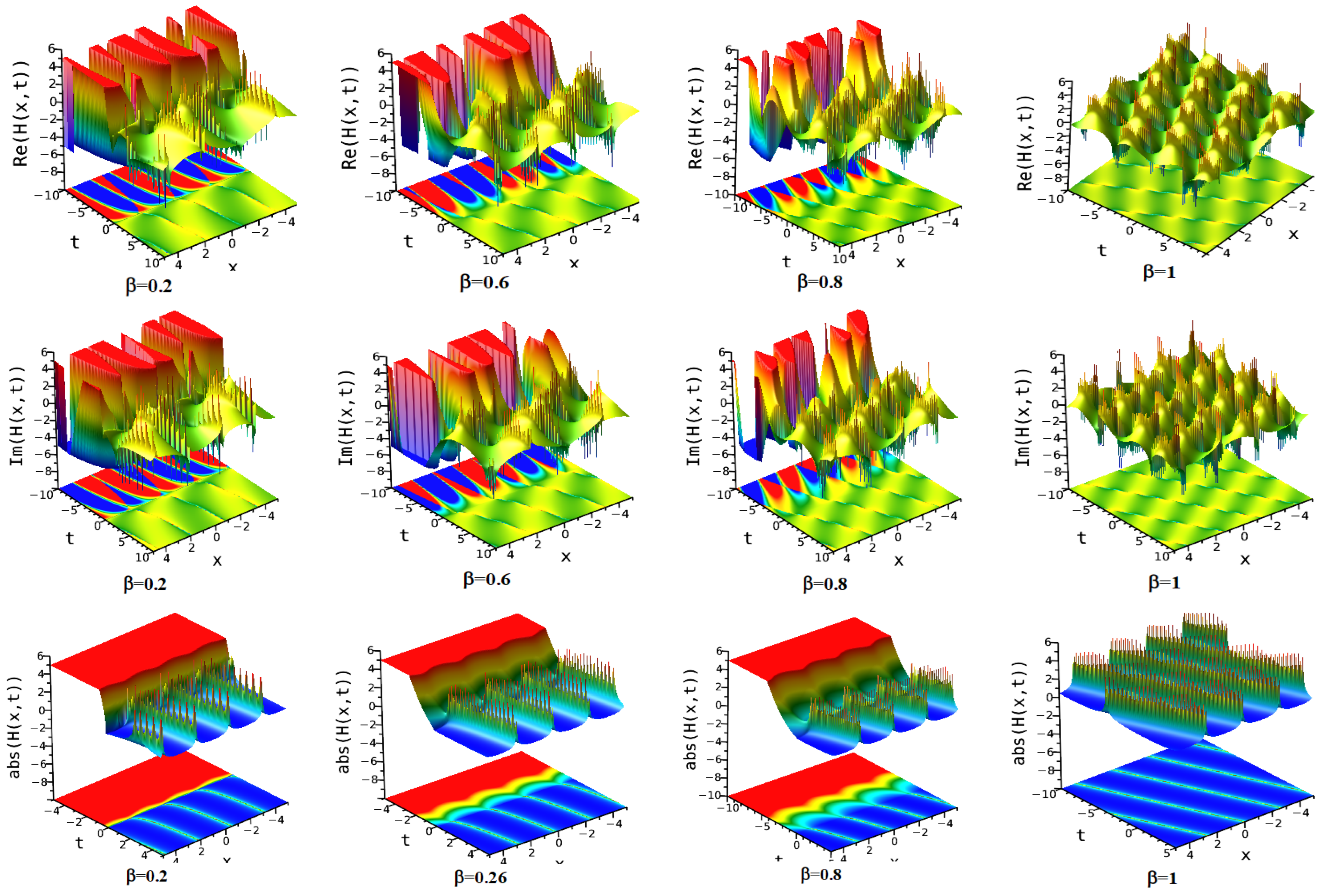
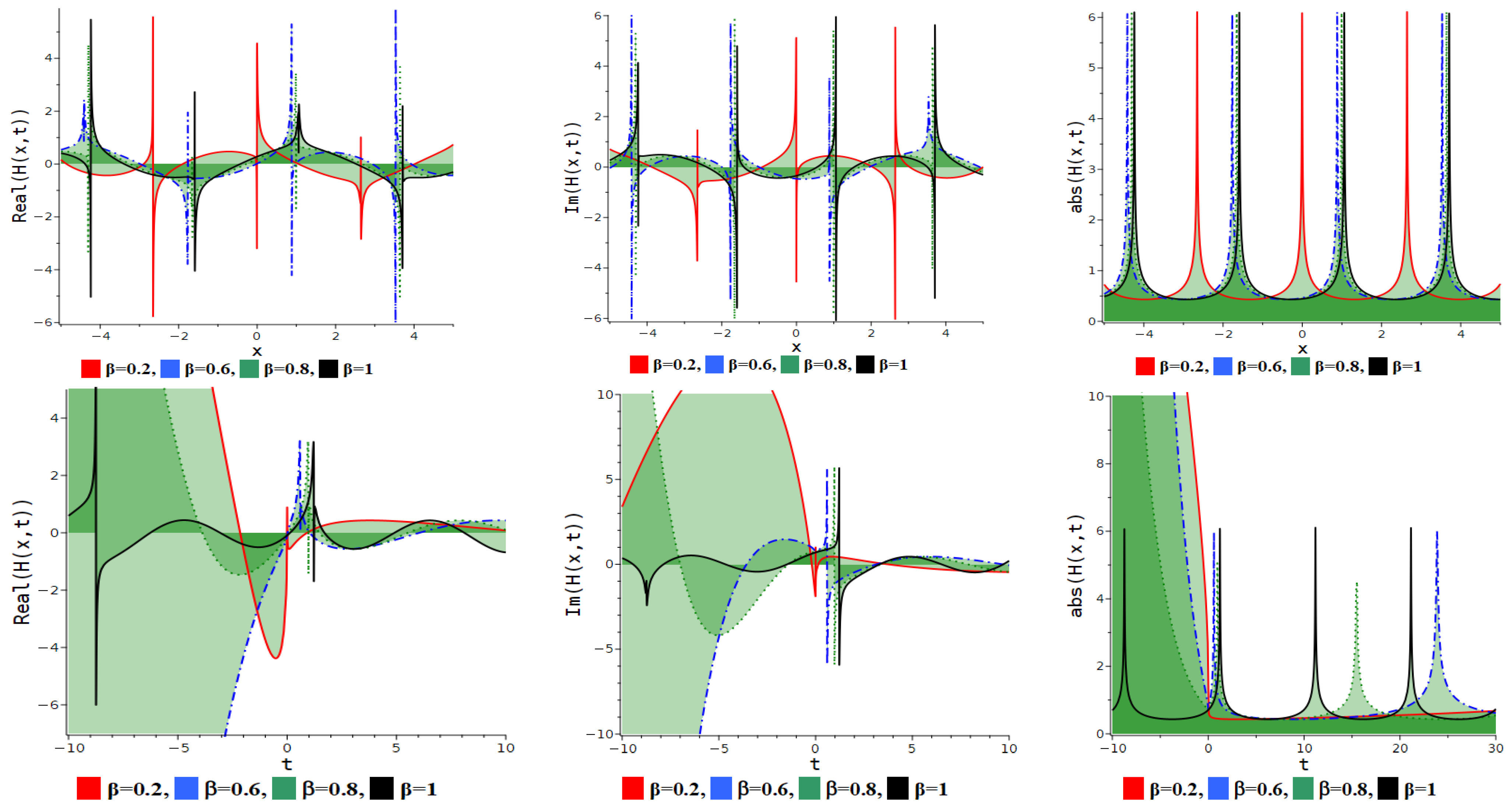
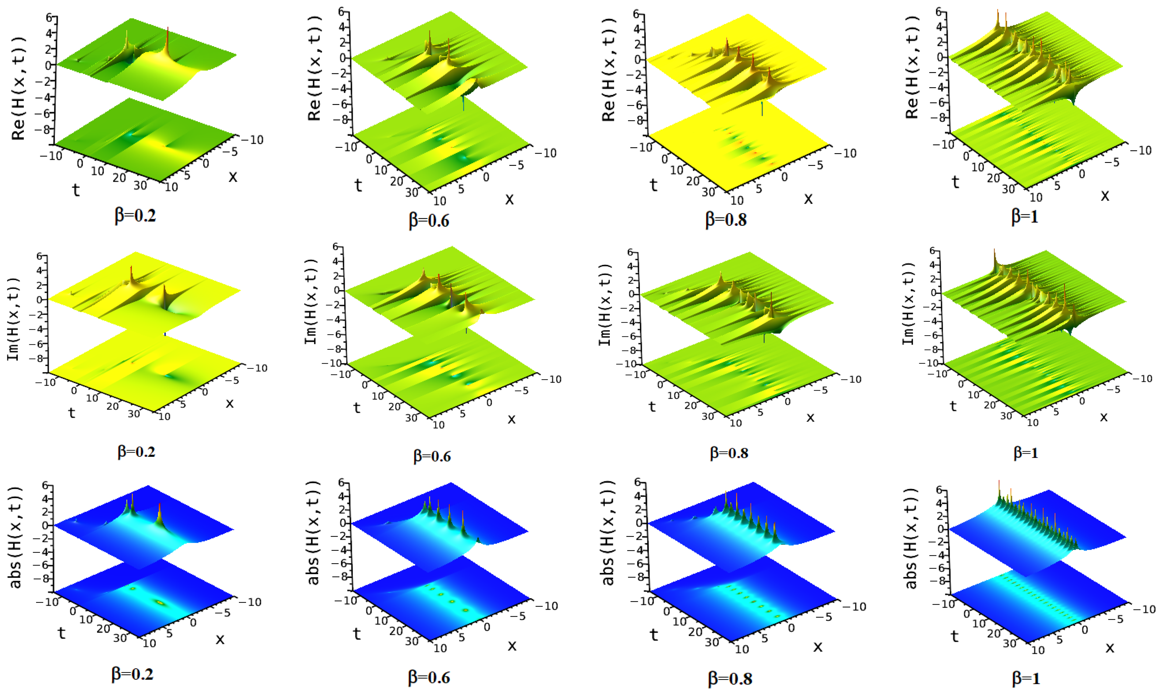
7. Numerical Discussion and Graphs

This study provides both dynamical behaviors using bifurcation theory and exact optical soliton solutions using the METH and SE techniques to the QKE equation with the M-fractional derivative. The derived solutions include many solitary wave types, such as exponential, rational, trigonometric, and hyperbolic functions. The bifurcation analysis of the quintic Kundu-Eckhaus (QKE) equation is essential for comprehending nonlinear wave dynamics in optics, fluids, and Bose–Einstein condensates. It categorizes soliton structures, forecasts stability and modulational instability, and delineates transitions among dynamical states. This study facilitates the identification of chaos and critical thresholds in wave evolution through two-dimensional phase portraits and stable circles in Figure 1, Figure 2, Figure 3, Figure 4, Figure 5 and Figure 6. It also facilitates the optimization of pulse propagation in optical fibers and the modeling of capillary waves in fluids. It mathematically advances the examination of QKE equations, offering insights into integrability and symmetry-breaking processes. It is crucial for theoretical progress and practical implementations in nonlinear wave physics. In Figure 7, Figure 8, Figure 9, Figure 10, Figure 11, Figure 12, Figure 13, Figure 14, Figure 15, Figure 16, Figure 17, Figure 18, Figure 19, Figure 20 and Figure 21, we also present some novel optical wave patterns of the derived solution for the special ideals of free parameters. The three-dimensional and two-dimensional diagrams illustrate the effect of M-fractional parameters on the obtained wave solutions. We compare the effect of M-fraction parameters with the original form of the derived solutions for the QKE equation with the values $\beta =0.2, 0.6, 0.8$.

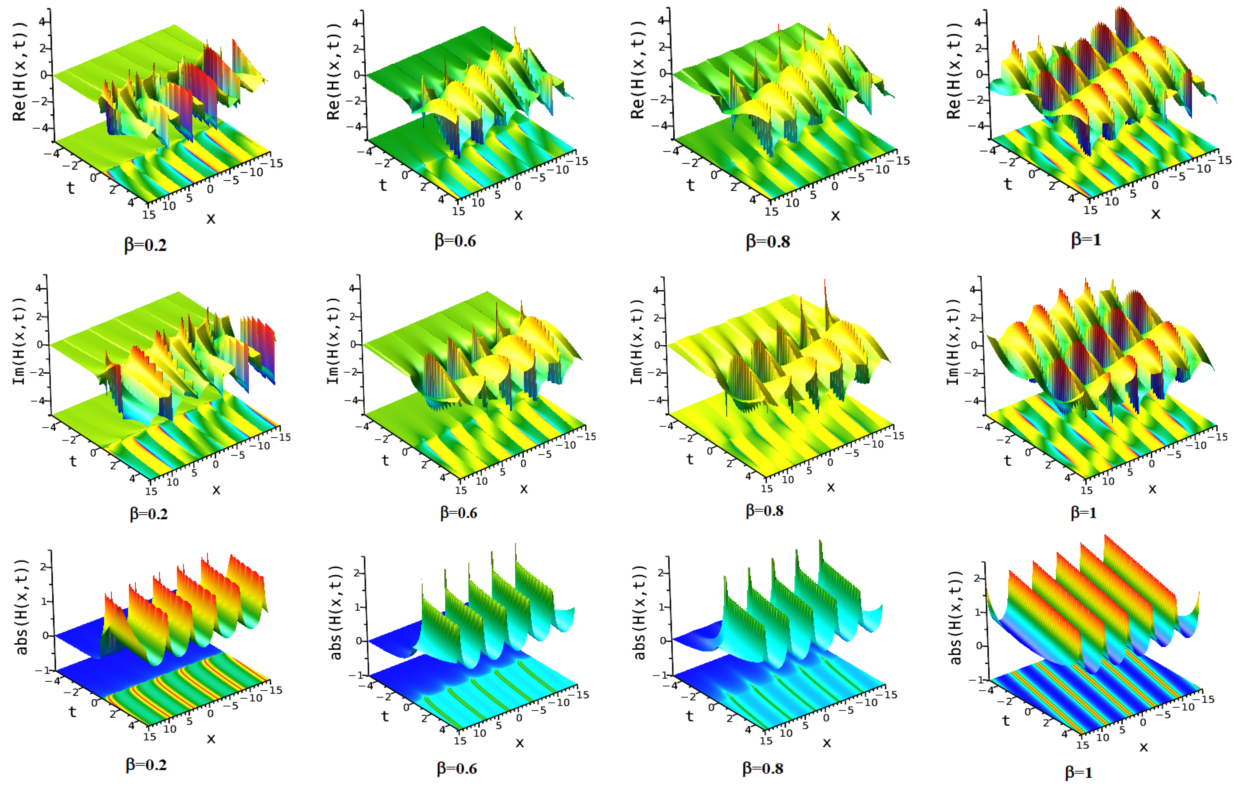
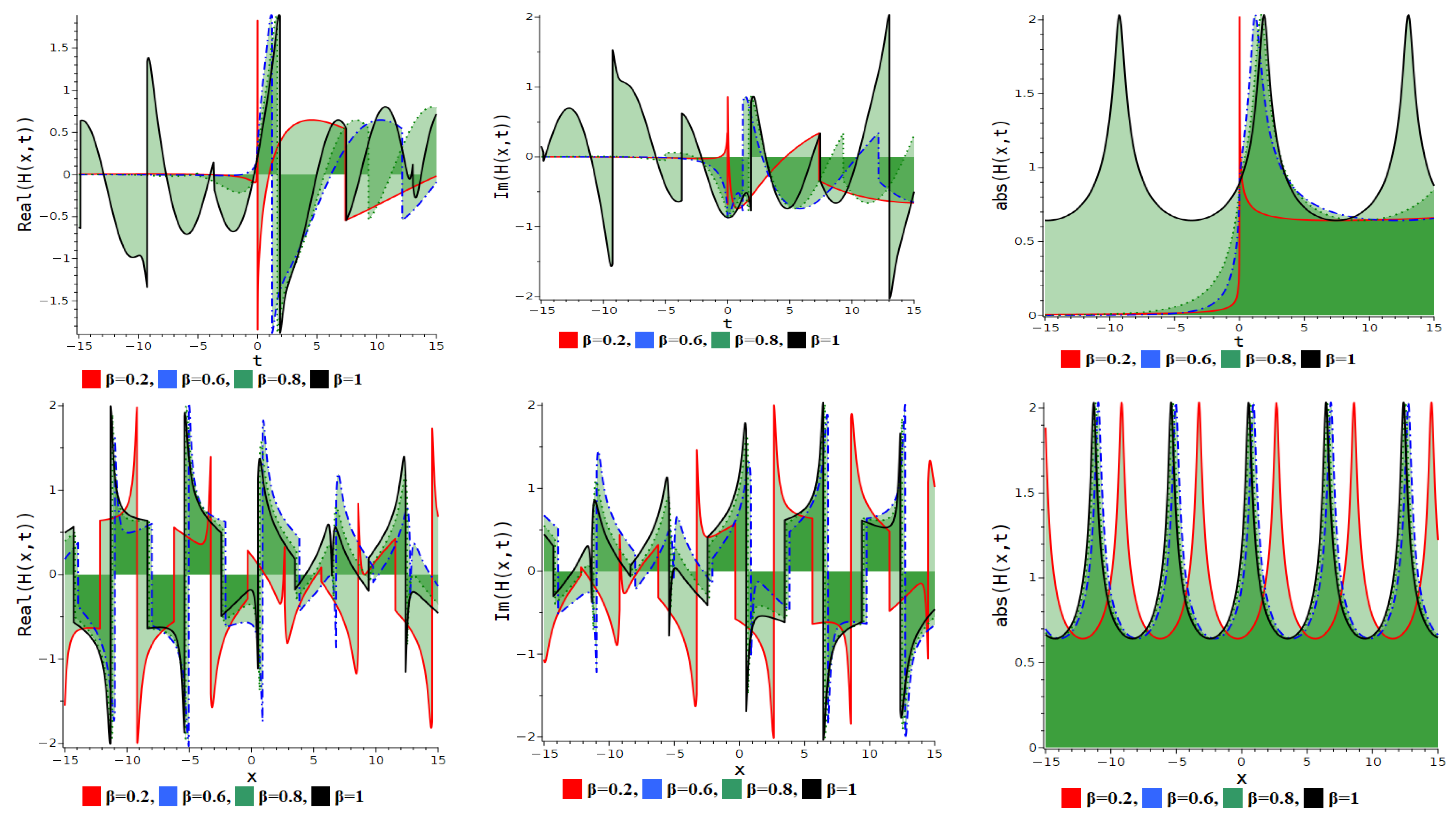
7.1. Modified Extended Tanh Method

To comprehend the dynamics of the results, one must understand the physical explanation of the acquired solutions. This section presents visual representations of the solutions we developed, utilizing three-dimensional density plots and two-dimensional plots to elucidate our findings. Given that the QKE equation is analogous to the Schrödinger equation, we concentrate on three fundamental elements: the real, imaginary, and absolute values of the resultant solutions. Utilizing the modified extended Tanh method, we illustrate various profiles of kinky periodic waves with dark characteristics, periodic breather waves, anti-kinky periodic waves with dark characteristics, periodic waves, multi-kink shape waves, and others. These profiles have significant applications in areas such as nonlinear optics, plasma physics, and fuzzy dynamics. Kinky periodic and anti-kinky periodic waves with dark properties show changes between separate wave states. This is important for understanding nonlinear domain walls, optical switching, and phase transitions in condensed matter systems and fiber optics. Periodic breather waves demonstrate confined energy oscillations, which are imperative in optical rogue waves and pulsing solitons that happen in nonlinear waveguides and hydrodynamics. Periodic waves make it easier to look at comprehensible wave patterns in nonlinear media, which changes how optical signals are sent and how plasma waves travel. The multi-kink shape wave model helps us understand how solitons collide and interact, giving us clues about how energy moves and how things stay stable in nonlinear dispersive media. Figure 11 depicts three-dimensional plots with density plots of the solution to Equation (15), which signifies a periodic breather wave soliton. The graphic is produced for particular parametric values, namely $A=-2, \mathsf{\Theta }=-1, l=0.1, B=-1.5, p=0.1, E=1, \theta =-0.1, \mu =1, and n=1.3$, illustrating the soliton’s structural attributes and wave dynamics. The fractional parametric ($\beta$) effect is also shown in this figure for $\beta =0.2, 0.6, and 0.8$, and without fractional form, we plotted a diagram for $\beta =1$. The real and imaginary parts depict the periodic breather waves, and the absolute part depicts the kinky periodic waves with dark characteristics. Figure 12 is presented alongside the associated two-dimensional projection of Figure 11. Here, we provide a comparative diagram of the fractional derivative and the classical form of the solution in Equation (15). Figure 13 illustrates the three-dimensional representations alongside density charts of the solution to Equation (15), indicating a periodic breather wave soliton. The graphic is generated for specific parametric values, namely $A=2, \mathsf{\Theta }=-1, l=0.1, B=1.5, p=0.1, E=0.5, \theta =0.1, \mu =1, and n=1.3$, depicting the soliton’s structural characteristics and wave dynamics. The fractional parametric $\left(\beta \right)$ impact is illustrated in this figure for $\beta$ values of 0.2, 0.6, and 0.8 beside a diagram for $\beta =1$ without the fractional form. The real and imaginary components illustrate the periodic breather waves, whereas the absolute component represents the anti-kinky periodic waves with dark attributes. Figure 14 is displayed alongside the corresponding two-dimensional projection of Figure 13. Here, we provide a comparative diagram of the fractional derivative and the classical form of the solution in Equation (15). Figure 15 explains the three-dimensional representations alongside density charts of the solution to Equation (18), indicating a periodic wave soliton. The graphic is generated for specific parametric values, namely $A=0.5, \mathsf{\Theta }=1, l=-0.1, B=0.5, p=1, E=1, \theta =-0.1, \mu =1, and n=1.3$, depicting the soliton’s structural characteristics and wave dynamics. The fractional parametric $\left(\beta \right)$ impact is illustrated in this figure for $\beta$ values of 0.2, 0.6, and 0.8 beside a diagram for $\beta =1$ that is the classical form. The real and imaginary components illustrate the periodic waves, whereas the absolute component represents the kinky periodic waves with dark attributes. Figure 16 is displayed alongside the corresponding two-dimensional projection of Figure 11. Here, we provide a comparative diagram of the fractional derivative and the classical form of the solution in Equation (18). Figure 17 illustrates the three-dimensional plots alongside density plots of the solution to Equation (20), indicating a periodic wave soliton for the values $A=2, \mathsf{\Theta }=-1, l=0.1, B=1.5, v=0.1, E=3, \theta =-0.1, \mu =1, n=1.3$. The fractional parametric $\left(\beta \right)$ impact is illustrated in this figure for $\beta$ values of 0.2, 0.6, and 0.8 beside a diagram for $\beta =1$ without the fractional form. The real and imaginary components illustrate the periodic waves, whereas the absolute component signifies the multi-kink shape waves. Figure 18 is displayed alongside the corresponding two-dimensional projection of Figure 18. Here, we provide a comparative diagram of the fractional derivative and the classical form of the solution in Equation (20).

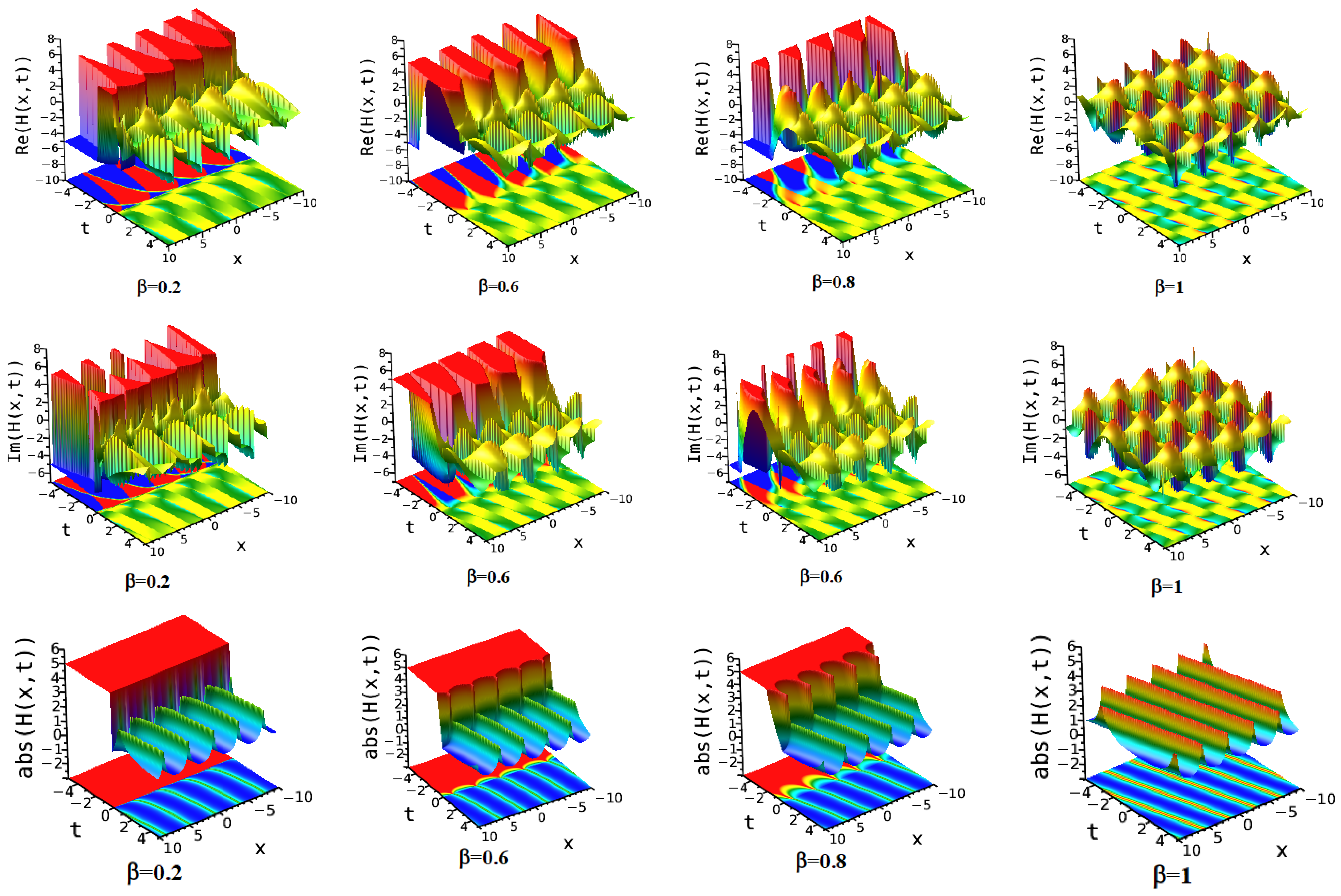
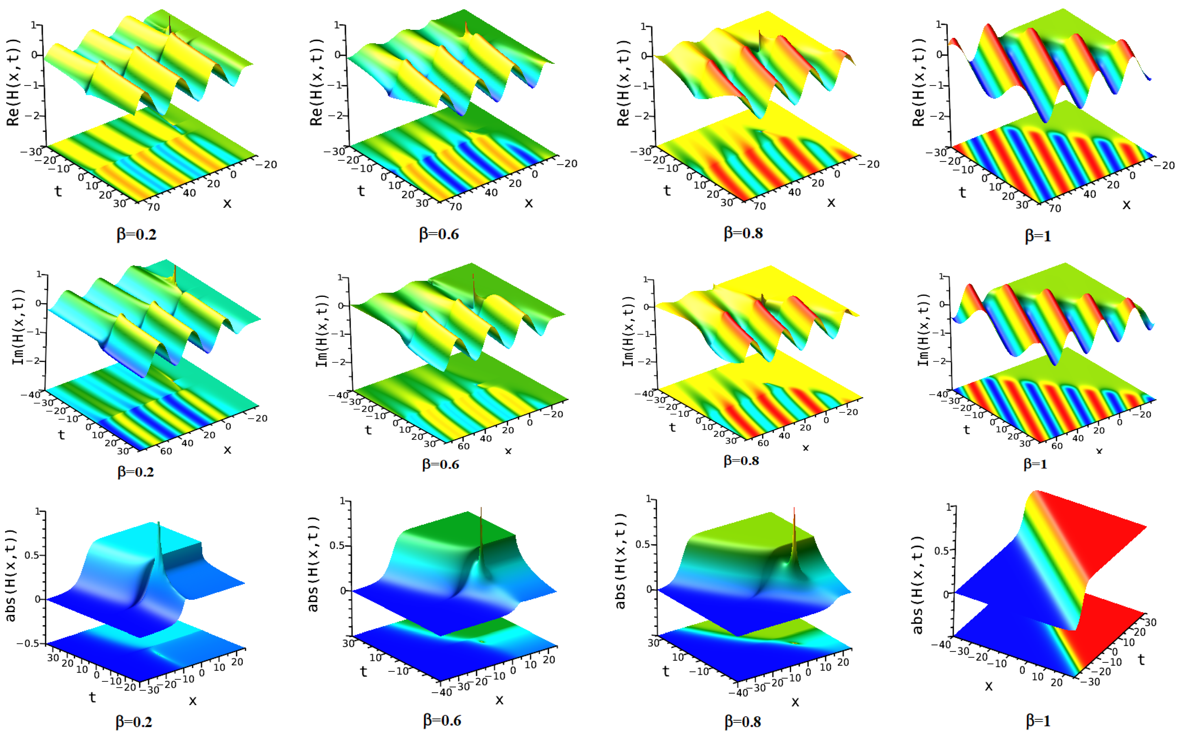
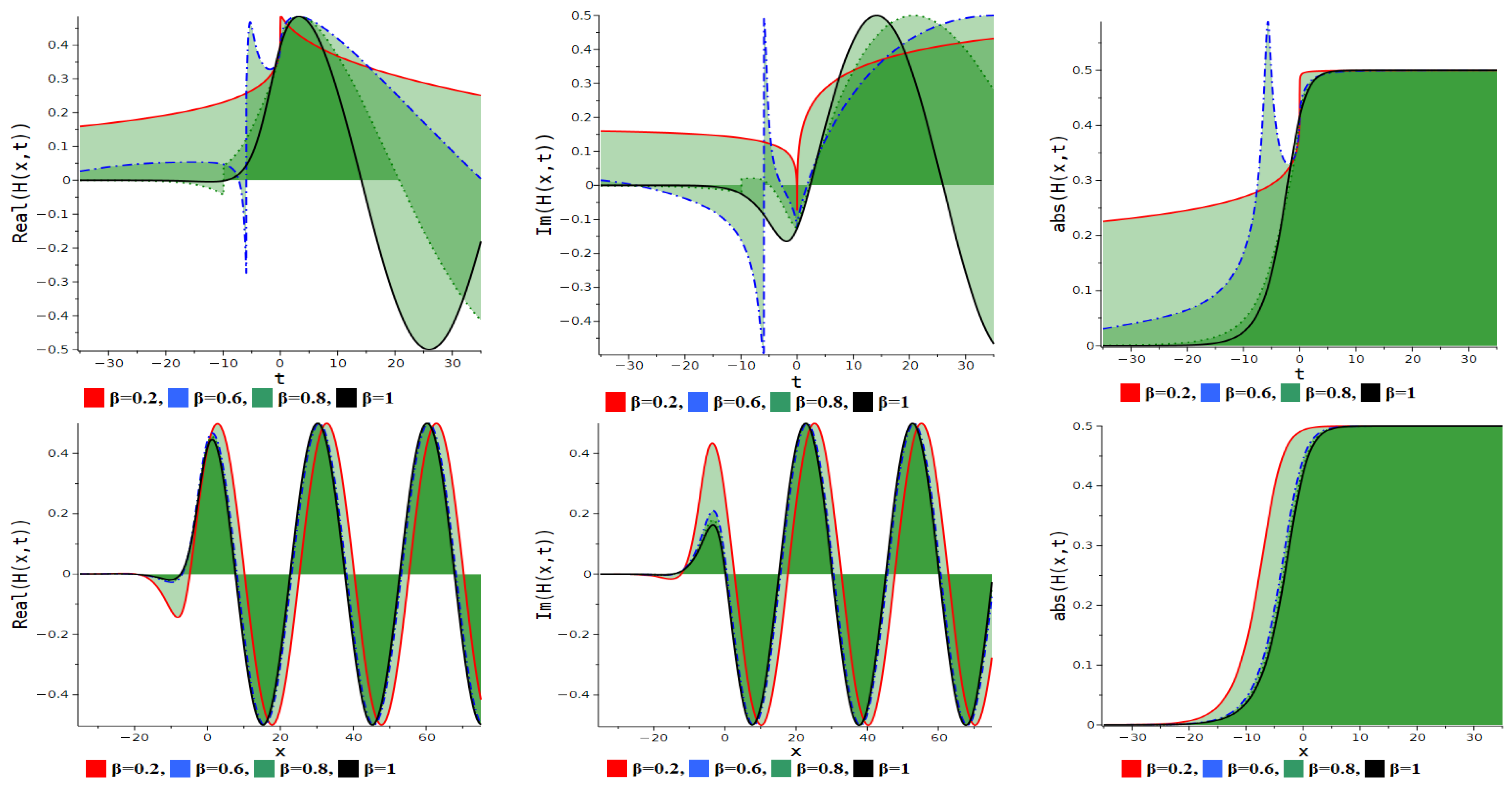
7.2. Simplest Equation Method

This section presents a visual analysis of the acquired solutions through 3D density and 2D charts. Given that the QKE equation parallels the Schrödinger equation, we analyze the real, imaginary, and absolute values of the solutions. Utilizing the modified extended Tanh approach, we demonstrate a range of soliton profiles, encompassing periodic breather waves, anti-kinky periodic waves with bright attributes, periodic lump wave soliton, and bright–dark double periodic waves. These structures are utilized in nonlinear optics, plasma physics, and fuzzy dynamics, facilitating light modulation and the comprehension of turbulence in chaotic systems. Periodic breather waves provide confined amplitude oscillations, crucial for comprehending rogue waves, energy localization, and pulse propagation in nonlinear optical systems. They assist in modeling transient energy concentration and recurring events. Periodic shifts between several bright soliton states are shown by anti-kinky periodic waves with luminous properties. These waves are significant for optical switching processes, nonlinear domain wall configurations, and plasma wave behavior. Periodic lump wave solitons are confined, non-singular structures that stay stable over long distances. They are very important in plasma physics, optical communication, and fluid dynamics, all of which involve multidimensional wave interactions. Bright–dark double periodic waves show how areas of high and low intensity (bright) interact in nonlinear media. They make it easier to study optical waveguides, fiber lasers, and the dynamics of matter waves in Bose–Einstein condensates. Figure 19 depicts three-dimensional plots with density plots of the solution to Equation (24), which signifies a periodic wave and breather wave soliton. The graphic is produced for particular parametric values, namely $A=-2, {\mathsf{\Theta }}_1=1, {\mathsf{\Theta }}_2=-0.5, l=0.1, B=-1.5, p=0.1, E=1, \theta =-0.1, \mu =1, and n=1.3$, illustrating the soliton’s structural attributes and wave dynamics. The fractional parametric ($\beta$) effect is also shown in this figure for $\beta =0.2, 0.6, and 0.8$, and without fractional form, we plotted a diagram for $\beta =1$. The real and imaginary parts depict the periodic wave with breather waves, and the absolute part depicts the bright–dark double periodic waves. Figure 20 is presented alongside the associated two-dimensional projection of Figure 19. Here, we provide a comparative diagram of the fractional derivative and the classical form of the solution in Equation (24). Figure 21 illustrates the three-dimensional representations alongside density charts of the solution to Equation (26), indicating a periodic breather wave soliton for $A=-0.1, {\mathsf{\Theta }}_1=-0.5, {\mathsf{\Theta }}_2=-1, l=-0.02, B=3, p=-1, E=1, \theta =0.1, and n=1.3$. The fractional parametric $\left(\beta \right)$ impact is illustrated in this figure for $\beta$ values of 0.2, 0.6, and 0.8 beside a diagram for $\beta =1$ without the fractional form. The real and imaginary components illustrate the periodic breather waves, whereas the absolute component represents the anti-kinky periodic waves with bright attributes. Figure 22 is displayed alongside the corresponding two-dimensional projection of Figure 22. Here, we provide a comparative diagram between the fractional derivative and the classical form of the solution in Equation (26).

Figure 23 explains the three-dimensional representations alongside density charts of the solution to Equation (31), indicating a periodic lump wave soliton. The graphic is generated for specific parametric values, namely $A=-1, {\mathsf{\Theta }}_1=-0.5, {\mathsf{\Theta }}_2=-1, l=0.1, B=-0.5, v=2, E=0.2, \theta =-0.1, \mu =1, and n=1.3$, depicting the soliton’s structural characteristics and wave dynamics. The fractional parametric $\left(\beta \right)$ impact is illustrated in this figure for $\beta$ values of 0.2, 0.6, and 0.8 beside a diagram for $\beta =1$ that is the classical form. The real and imaginary components illustrate the periodic lump waves, whereas the absolute component represents the periodic lump waves with dark attributes. Figure 24 is displayed alongside the corresponding two-dimensional projection of Figure 23. Here, we provide a comparative diagram between the fractional derivative and the classical form of the solution in Equation (31).

8. Conclusions

The examination of the QKE equation establishes a theoretical basis for signal transmission in contemporary optical systems intended for ultrafast communication and high-density data storage. Optical solitons and their related effects are essential for enabling effective and dependable data transfer. Engineers can optimize system designs to improve communication performance and storage efficiency by analyzing diverse alternatives. Soliton solutions facilitate high-speed data transmission, periodic solutions are essential for multi-channel communication, and solitary and unbounded solutions contribute to the development of interference-resistant systems. In this manuscript, the dynamical behaviors of the QKE equation were successfully analyzed by using bifurcation analysis with the two-dimensional phase portrait. In Figure 1, Figure 2, Figure 3, Figure 4, Figure 5 and Figure 6, the stable circle and phase portraits are presented. We showed the stable and unstable critical points under some parametric conditions. This study examined optical solitons in the QKE equation, integrating fractional temporal evolution. Employing the modified extended Tanh and simplest equation techniques, a complete soliton spectrum was derived, accompanied by the requisite parameter conditions for their existence. The soliton spectrums are periodic breather waves, anti-kinky periodic waves with bright attributes, periodic lump wave solitons, bright–dark double periodic waves, kinky periodic waves with dark characteristics, anti-kinky periodic waves with dark characteristics, periodic waves, and multi-kink shape waves, which are presented in Figure 7, Figure 8, Figure 9, Figure 10, Figure 11, Figure 12, Figure 13, Figure 14, Figure 15, Figure 16, Figure 17, Figure 18, Figure 19 and Figure 20 with 3D and 2D diagrams. The retrieved solutions exhibit considerable potential for alleviating internet congestion. The fractional parametric ($\beta$) effect on the optical solitons is also shown in Figure 7, Figure 8, Figure 9, Figure 10, Figure 11, Figure 12, Figure 13, Figure 14, Figure 15, Figure 16, Figure 17, Figure 18, Figure 19 and Figure 20 for $\beta =0.2, 0.6, 0.8$, and we plotted the classical form of these solitons for $\beta =1$. The findings establish a robust basis for further studies, encompassing an examination of the dispersive concatenation model, anticipated to produce analogous answers.

References

1. Gu, Y.; Chen, B.; Ye, F.; Aminakbari, N. Soliton Solutions of Nonlinear Schrödinger Equation with Variable Coefficients under the Influence of Woods–Saxon Potential. Results Phys. 2022, 42, 105979. [Google Scholar] [CrossRef]
2. Chen, J.; Mihalache, D.; Belić, M.R.; Qin, W.; Zhu, D.; Zhu, X.; Zeng, L. Dark Gap Soliton Families in Coupled Nonlinear Schrödinger Equations with Linear Lattices. Nonlinear Dyn. 2024, 113, 10307–10318. [Google Scholar] [CrossRef]
3. Roshid, M.M.; Rahman, M.; Sheikh, M.A.N.; Uddin, M.; Khatun, M.S.; Roshid, H.O. Dynamical Analysis of Multi-Soliton and Interaction of Soliton Solutions of Nonlinear Model Arising in Energy Particles of Physics. Indian J. Phys. 2025, 2025, 1–13. [Google Scholar]
4. Ganie, A.H.; AlBaidani, M.M.; Wazwaz, A.M.; Ma, W.X.; Shamima, U.; Ullah, M.S. Soliton Dynamics and Chaotic Analysis of the Biswas–Arshed Model. Opt. Quant. Electron. 2024, 56, 1379. [Google Scholar] [CrossRef]
5. Akter, M.; Ullah, M.S.; Wazwaz, A.M.; Seadawy, A.R. Unveiling Hirota–Maccari Model Dynamics via Diverse Elegant Methods. Opt. Quant. Electron. 2024, 56, 1127. [Google Scholar] [CrossRef]
6. Akter, M.A.; Mostafa, G.; Uddin, M.; Roshid, M.M.; Roshid, H.O. Simulation of Optical Wave Propagation of Perturbed Nonlinear Schrödinger’s Equation with Truncated M-Fractional Derivative. Opt. Quant. Electron. 2024, 56, 1255. [Google Scholar] [CrossRef]
7. Roshid, M.M. Exploring the Chaotic Behavior, and Ion Acoustic Wave of Generalized Perturbed Korteweg-de Vries Equation with a Fractional Operator. Partial Differ. Equ. Appl. Math. 2024, 13, 101042. [Google Scholar] [CrossRef]
8. Shah, Z.; Raja, M.A.Z.; Shoaib, M.; Khan, I.; Kiani, A.K. Stochastic Supervised Networks for Numerical Treatment of Eyring–Powell Nanofluid Model with Darcy Forchheimer Slip Flow Involving Bioconvection and Nonlinear Thermal Radiation. Mod. Phys. Lett. B 2025, 39, 2450400. [Google Scholar] [CrossRef]
9. Wazwaz, A.M.; Alhejaili, W.; El-Tantawy, S.A. Optical Solitons for Nonlinear Schrödinger Equation Formatted in the Absence of Chromatic Dispersion through Modified Exponential Rational Function Method and Other Distinct Schemes. Ukr. J. Phys. Opt. 2024, 25, 1049–1059. [Google Scholar] [CrossRef]
10. Butler, S.; Joshi, N. An Inverse Scattering Transform for the Lattice Potential KdV Equation. Inverse Probl. 2010, 26, 115012. [Google Scholar] [CrossRef]
11. Kazi Sazzad Hossain, A.K.M.; Kamrul Islam, M.; Akter, H.; Ali Akbar, M. Exact and Soliton Solutions of Nonlinear Evolution Equations in Mathematical Physics Using the Generalized (G′/G)-Expansion Approach. Phys. Scr. 2024, 99, 015269. [Google Scholar] [CrossRef]
12. Seadawy, A.R. Fractional Solitary Wave Solutions of the Nonlinear Higher-Order Extended KdV Equation in a Stratified Shear Flow: Part I. Comput. Math. Appl. 2015, 70, 345–352. [Google Scholar] [CrossRef]
13. Biswas, A.; Yıldırım, Y.; Yaşar, E. Optical Soliton Perturbation with Quadratic-Cubic Nonlinearity by Extended Trial Function Method. Optik 2019, 176, 542–548. [Google Scholar] [CrossRef]
14. Wang, K.-J.; Liu, X.-L.; Shi, F.; Li, G. Bifurcation and Sensitivity Analysis, Chaotic Behaviors, Variational Principle, Hamiltonian and Diverse Wave Solutions of the New Extended Integrable Kadomtsev–Petviashvili Equation. Phys. Lett. A 2025, 534, 130246. [Google Scholar] [CrossRef]
15. Ahmed, S.; Rehman, U.; Fei, J.; Khalid, M.I.; Chen, X. Shallow-Water Wave Dynamics: Butterfly Waves, X-Waves, Multiple-Lump Waves, Rogue Waves, Stripe Soliton Interactions, Generalized Breathers, and Kuznetsov–Ma Breathers. Fractal Fract. 2025, 9, 31. [Google Scholar] [CrossRef]
16. Arnous, A.H.; Murad, M.A.S.; Biswas, A.; Yildirim, Y.; Georgescu, P.L.; Moraru, L.; Jawad, A.J.M.; Hussein, L. Optical Solitons for the Concatenation Model with Fractional Temporal Evolution. Ain Shams Eng. J. 2025, 16, 103243. [Google Scholar] [CrossRef]
17. Iqbal, M.A.; Gepreel, K.A.; Akbar, M.A.; Osman, M.S. The Compatibility and Dynamics of Optical Soliton Solutions for Higher-Order Nonlinear Schrödinger Model. Mod. Phys. Lett. B 2024, 39, 2550086. [Google Scholar] [CrossRef]
18. Chou, D.; Boulaaras, S.M.; Rehman, H.U.; Iqbal, I.; Ma, W.-X. Multiple Soliton and Singular Wave Solutions with Bifurcation Analysis for a Strain Wave Equation Arising in Microcrystalline Materials. Mod. Phys. Lett. B 2025, 39, 2150031. [Google Scholar] [CrossRef]
19. Alhejaili, W.; Wazwaz, A.-M.; El-Tantawy, S.A. Extended New Painlevé Integrable KdV–CBS Equation: Multiple Shocks, Lump, Breathers, and Other Physical Wave Solutions. Phys. Scr. 2024, 99, 015269. [Google Scholar] [CrossRef]
20. Abbagari, S.; Houwe, A.; Akinyemi, L.; Serge, D.Y.; Crépin, K.T. Multi-Hump Soliton and Rogue Waves of the Coupled Nonlinear Schrödinger Equations in Nonlinear Left-Handed Transmission Line. Nonlinear Dyn. 2024, 98, 2024. [Google Scholar] [CrossRef]
21. Jawaz, M.; Macías-Díaz, J.E.; Aqeel, S.A.; Ahmed, N.; Baber, M.Z.; Medina-Guevara, M.G. On Some Explicit Solitary Wave Patterns for a Generalized Nonlinear Reaction–Diffusion Equation with Conformable Temporal Fractional Derivative. Partial Differ. Equ. Appl. Math. 2025, 13, 101036. [Google Scholar] [CrossRef]
22. Ma, W.X.; Geng, X. New Completely Integrable Neumann Systems Related to the Perturbation KdV Hierarchy. Phys. Lett. B 2024, 475, 56–62. [Google Scholar] [CrossRef]
23. Ma, W.X.; Zhou, R. On Inverse Recursion Operator and Tri-Hamiltonian Formulation for a Kaup-Newell System of DNLS Equations. J. Phys. A Math. Gen. 2024, 32, L239. [Google Scholar] [CrossRef]
24. Islam, M.S.; Roshid, M.M.; Uddin, M.; Ahmed, A. Modulation Instability and Dynamical Analysis of New Abundant Closed-Form Solutions of the Modified Korteweg–de Vries–Zakharov–Kuznetsov Model With Truncated M-Fractional Derivative. J. Appl. Math. 2024, 2024, 1754782. [Google Scholar] [CrossRef]
25. Djaouti, A.M.; Roshid, M.M.; Abdeljabbar, A.; Al-Quran, A. Bifurcation Analysis and Solitary Wave Solution of Fractional Longitudinal Wave Equation in Magneto-Electro-Elastic (MEE) Circular Rod. Results Phys. 2024, 64, 107918. [Google Scholar] [CrossRef]
26. Wazwaz, A.M. New Solitary Wave Solutions to the Kuramoto-Sivashinsky and the Kawahara Equations. Appl. Math. Comput. 2024, 182, 1642–1650. [Google Scholar] [CrossRef]
27. Liu, W.; Wazwaz, A.M.; Zheng, X. High-Order Breathers, Lumps, and Semi-Rational Solutions to the (2+1)-Dimensional Hirota–Satsuma–Ito Equation. Phys. Scr. 2024, 94, 075203. [Google Scholar] [CrossRef]
28. Chakrabarty, A.K.; Akter, S.; Uddin, M.; Roshid, M.M.; Abdeljabbar, A.; Or-Roshid, H. Modulation Instability Analysis, and Characterize Time-Dependent Variable Coefficient Solutions in Electromagnetic Transmission and Biological Field. Partial Differ. Equ. Appl. Math. 2024, 11, 100765. [Google Scholar] [CrossRef]
29. Ma, W.; Zhou, R. Binary Nonlinearization of Spectral Problems of the Perturbation AKNS Systems. Chaos Solitons Fractals 2002, 13, 1451–1463. [Google Scholar] [CrossRef]
30. Li, B.; Zhu, L. Turing Instability Analysis of a Reaction–Diffusion System for Rumor Propagation in Continuous Space and Complex Networks. Inf. Process. Manag. 2024, 61, 103621. [Google Scholar] [CrossRef]
31. Zhang, Z.; Wu, D.; Li, N. Predator Invasion in a Spatially Heterogeneous Predator-Prey Model with Group Defense and Prey-Taxis. Math. Comput. Simul. 2024, 226, 270–282. [Google Scholar] [CrossRef]
32. Yuan, T.; Guan, G.; Shen, S.; Zhu, L. Stability Analysis and Optimal Control of Epidemic-Like Transmission Model with Nonlinear Inhibition Mechanism and Time Delay in Both Homogeneous and Heterogeneous Networks. J. Math. Anal. Appl. 2023, 526, 127273. [Google Scholar] [CrossRef]
33. Ahmed, K.K.; Badra, N.M.; Ahmed, H.M.; Rabie, W.B. Soliton Solutions and Other Solutions for Kundu–Eckhaus Equation with Quintic Nonlinearity and Raman Effect Using the Improved Modified Extended Tanh-Function Method. Mathematics 2022, 10, 4203. [Google Scholar] [CrossRef]
34. Podlubny, I. Fractional Differential Equations; Academic Press: Cambridge, MA, USA, 1999. [Google Scholar]
35. Kilbas, A.A.; Srivastava, H.M.; Trujillo, J.J. Theory and Applications of Fractional Differential Equations; Elsevier: Amsterdam, The Netherlands, 2006. [Google Scholar]
36. Oldham, K.B.; Spanier, J. The Fractional Calculus: Theory and Applications of Differentiation and Integration to Arbitrary Order; Academic Press: Cambridge, MA, USA, 1974. [Google Scholar]
37. Samko, S.G.; Kilbas, A.A.; Marichev, O.I. Fractional Integrals and Derivatives: Theory and Applications; Gordon and Breach Science Publishers: London, UK, 1993. [Google Scholar]
38. Biswas, A.; Salah, M.B.H.; Zerrad, E. Optical Solitons in Fractional Domains. Appl. Math. Comput. 2016, 274, 208–213. [Google Scholar] [CrossRef]
39. Jumarie, G. Modified Riemann–Liouville Derivative and Fractional Taylor Series of Nondifferentiable Functions: Further Results. Math. Comput. Model. 2009, 51, 16–26. [Google Scholar] [CrossRef]
40. Alhejaili, W.; Shah, R.; Salas, A.H.; Raut, S.; Roy, S.; Roy, A.; El-Tantawy, S.A. Unearthing the Existence of Intermode Soliton-Like Solutions within Integrable Quintic Kundu–Eckhaus Equation. Rend. Lincei Sci. Fis. Nat. 2024, 36, 233–255. [Google Scholar] [CrossRef]
41. Roshid, H.-O.; Roshid, M.M.; Abdeljabbar, A.; Begum, M.; Basher, H. Abundant Dynamical Solitary Waves through Kelvin-Voigt Fluid via the Truncated M-Fractional Oskolkov Model. Results Phys. 2023, 55, 107128. [Google Scholar] [CrossRef]
42. Roshid, M.M.; Rahman, M.M.; Bashar, M.H.; Hossain, M.M.; Mannaf, M.A. Dynamical Simulation of Wave Solutions for the M-Fractional Lonngren-Wave Equation Using Two Distinct Methods. Alex. Eng. J. 2024, 81, 460–468. [Google Scholar] [CrossRef]
43. Roshid, M.M.; Uddin, M.; Hossain, M.M.; Roshid, H.-O. Investigation of Rogue Wave and Dynamic Solitary Wave Propagations of the M-Fractional (1+1)-Dimensional Longitudinal Wave Equation in a Magnetic-Electro-Elastic Circular Rod. Indian J. Phys. 2024, 99, 1787–1803. [Google Scholar] [CrossRef]
Figure 1. Phase portrait of system in Equation (6) for A = k = p = 1, v = 0.5, B = −0.5, E = 0.5.
Fractalfract 09 00334 g001
Figure 2. Phase portrait of system in Equation (6) for A = k = p = 1, v = −2.5, B = 0.5, E = −0.5.
Fractalfract 09 00334 g002
Figure 3. Phase portrait of system in Equation (6) for A = k = p = 1, v = −2.5, B = −0.5, E = −0.5.
Fractalfract 09 00334 g003
Figure 4. Phase portrait of system in Equation (6) for A = k = p = 1, v = −2.5, B = −0.5, E = 0.5.
Fractalfract 09 00334 g004
Figure 5. Phase portrait of system in Equation (6) for A = k = p = 1, v = 0.5, B = 0.5, E = −0.5.
Fractalfract 09 00334 g005
Figure 6. Phase portrait of system in Equation (6) for A = k = p = 1, v = −2.5, B = −0.5, E = −0.5.
Fractalfract 09 00334 g006
Figure 7. Numerical solution and sensitivity as A takes greater value of system in Equation (7) for K = 1, A = 1, p = 1, v = −2.5, B = −0.5, E = −0.5: (a) sensitivity in 2D shape, (b) 3D phase plot, (c) 2D phase plot.
Fractalfract 09 00334 g007
Figure 8. Numerical solution and sensitivity as A takes a smaller value of the system in Equation (7) for K = 1, A = 0.1, p = 1, v = −2.5, B = −0.5, E = −0.5: (a) sensitivity in 2D shape, (b) 3D phase plot, (c) 2D phase plot.
Fractalfract 09 00334 g008aFractalfract 09 00334 g008b
Figure 9. Asymptotically unstable and sensitivity of system in Equation (7) for K = 1, A = 1, p = 1, v = −2.5, B = −0.5, E = 0.5: (a) sensitivity in 2D shape, (b) 3D phase plot, (c) 2D phase plot.
Fractalfract 09 00334 g009
Figure 10. Asymptotical stability and sensitivity of system in Equation (7) for K = 1, A = 1, p = 1, v = −2.5, B = −0.5, E = 0.5: (a) sensitivity in 2D shape, (b) 3D phase plot, (c) 2D phase plot.
Fractalfract 09 00334 g010
Figure 11. Three-dimensional profile of solution for Equation (15), plotted in (x,t)-plane for A = −2, Θ = −1, l = 0.1, B = −1.5, p = 0.1, E = 1, θ = −0.1, μ = 1, n = 1.3.
Fractalfract 09 00334 g011
Figure 12. Two-dimensional profiles of the solution for Equation (15) plotted along x-axis and t-axis.
Fractalfract 09 00334 g012
Figure 13. Three-dimensional profile of solution for Equation (15) plotted in (x,t)-plane for A = 2, Θ = −1, l = 0.1, B = 1.5, p = 0.1, E = 0.5, θ = 0.1, μ = 1, n = 1.3.
Fractalfract 09 00334 g013
Figure 14. Two-dimensional profiles of the solution for Equation (15) plotted along x-axis and t-axis.
Fractalfract 09 00334 g014
Figure 15. Three-dimensional profile of solution for Equation (18) plotted in (x,t)-plane for A = 0.5, Θ = 1, l = −0.1, B = 0.5, p = 1, E = 1, θ = −0.1, μ = 1, n = 1.3.
Fractalfract 09 00334 g015
Figure 16. Two-dimensional profile of solution for Equation (18) plotted along x-axis and t-axis.
Fractalfract 09 00334 g016
Figure 17. Three-dimensional profile of solution for Equation (20) plotted in (x,t)-plane for A = 2, Θ = −1, l = 0.1, B = 1.5, v = 0.1, E = 3, θ = −0.1, μ = 1, n = 1.3.
Fractalfract 09 00334 g017
Figure 18. Two-dimensional profile of solution for Equation (20) plotted along x-axis and t-axis.
Fractalfract 09 00334 g018
Figure 19. Three-dimensional profile of solution for Equation (24) plotted in (x,t)-plane for A = −2, Θ1 = 1, Θ2 = −0.5, l = 0.1, B = −1.5, p = 0.1, E = 1, θ = −0.1, μ = 1, n = 1.3.
Fractalfract 09 00334 g019
Figure 20. Two-dimensional profile of solution for Equation (24) plotted along x-axis and t-axis.
Fractalfract 09 00334 g020
Figure 21. Three-dimensional profile of solution for Equation (26) plotted in (x,t)-plane for A = −0.1, Θ1 = −0.5, Θ2 = −1, l = −0.02, B = 3, p = −1, E = 1, θ = 0.1, n = 1.3.
Fractalfract 09 00334 g021
Figure 22. Two-dimensional profile of solution for Equation (26) plotted along x-axis and t-axis.
Fractalfract 09 00334 g022
Figure 23. Three-dimensional profile of solution for Equation (31) plotted in (x,t)-plane for A = −1, Θ1 = −0.5, Θ2 = −1, l = 0.1, B = −0.5, v = 2, E = 0.2, θ = −0.1, μ = 1, n = 1.3.
Fractalfract 09 00334 g023
Figure 24. Two-dimensional profile of the solution for Equation (31) plotted along x-axis and t-axis.
Fractalfract 09 00334 g024
Disclaimer/Publisher’s Note: The statements, opinions and data contained in all publications are solely those of the individual author(s) and contributor(s) and not of MDPI and/or the editor(s). MDPI and/or the editor(s) disclaim responsibility for any injury to people or property resulting from any ideas, methods, instructions or products referred to in the content.